Numerical Simulation of Sheet Metal Forming Using Non-Associated Flow Rule and Mixed Isotropic-Nonlinear Kinematic Hardening Model

University of Windsor University of Windsor

Scholarship at UWindsor

Scholarship at UWindsor

Electronic Theses and Dissertations Theses, Dissertations, and Major Papers

2010

Numerical Simulation of Sheet Metal Forming Using

Numerical Simulation of Sheet Metal Forming Using

Non-Associated Flow Rule and Mixed Isotropic-Nonlinear Kinematic

Associated Flow Rule and Mixed Isotropic-Nonlinear Kinematic

Hardening Model

Hardening Model

Aboozar Taherizadeh University of Windsor

Follow this and additional works at: https://scholar.uwindsor.ca/etd

Recommended Citation Recommended Citation

Taherizadeh, Aboozar, "Numerical Simulation of Sheet Metal Forming Using Non-Associated Flow Rule and Mixed Isotropic-Nonlinear Kinematic Hardening Model" (2010). Electronic Theses and Dissertations. 468.

https://scholar.uwindsor.ca/etd/468

Numerical Simulation of Sheet Metal Forming Using

Non-Associated Flow Rule and Mixed Isotropic-

Nonlinear Kinematic Hardening Model

by

Aboozar Taherizadeh

A Dissertation

Submitted to the Faculty of Graduate Studies through Mechanical Engineering in Partial Fulfillment of the Requirements for

the Degree of Doctor of Philosophy at the University of Windsor

Windsor, Ontario, Canada 2009

Numerical Simulation of Sheet Metal Forming Using Non-Associated Flow Rule and Mixed Isotropic- Nonlinear Kinematic Hardening Model

by

Aboozar Taherizadeh

APPROVED BY:

______________________________ Dr. P. Wu, External Examiner

Department of Mechanical Engineering, McMaster University

______________________________ Dr. D. Green, Advisor

Mechanical Engineering (MAME)

______________________________ Dr. W. Altenhof, Co-advisor

Mechanical Engineering (MAME)

______________________________ Dr. N. Zamani, Department Reader Mechanical Engineering (MAME)

______________________________ Dr. D. Watt, Department Reader Engineering Materials (MAME)

______________________________ Dr. S. Das, Outside Reader

Civil and Environmental Engineering

______________________________ Dr. W. ElMaraghy, Chair of Defense

Declaration of Co-Authorship/Previous Publication

I. Co-Authorship Declaration

I hereby declare that this dissertation incorporates material that is result of joint research, as follows:

• Uniaxial tensile tests for 3 steel sheets used in Chapter 3, 4 and 5 were carried out by

Ming Shi from United States Steel and Mai Huang from Mittal Steel.

• Uniaxial tensile tests and biaxial bulge tests for the aluminum alloy used in Chapter 3,

4 and 5 were carried out by J. Brem, F. Barlat, R. Dick and J.W. Yoon from Alcoa.

• Cyclic shear tests used in Chapter 3 and 4 were carried out by Professor S. Thuillier

from the Université de Bretagne-Sud in France.

• Hydraulic bulge tests on the steel sheets used in Chapter 3, 4 and 5 were carried out

by Dr. J-W Yoon from Alcoa.

• Cyclic tension-compression tests used in Chapter 5 were carried out by Professor

Wagoner and Piao Kun from the Ohio State University.

• Measurements of residual stresses used in Chapter 3 were carried out by Dr. T.

Gnaeupel-Herold from the NIST.

• Dr. Jean Reid from the IRDI in Midland, Ontario, was responsible for the

measurement of friction coefficients used in springback simulations in Chapter 3, 4 and 5.

• Numisheet’05 Benchmark #3 channel draw tests used in Chapter 3, 4 and 5 were

performed at the Industrial Research & Development Institute (IRDI) in Midland, Ontario. Also, General Motors of Canada sponsored the Numisheet’05 Benchmark #3 and the A/SP was responsible for building the channel draw die.

I am aware of the University of Windsor Senate Policy on Authorship and I certify that I have properly acknowledged the contribution of other researchers to my dissertation, and have obtained written permission from each of the co-author(s) to include the above material(s) in my dissertation.

II. Declaration of Previous Publication

This dissertation includes 3 original papers that have been previously published/submitted for publication in peer reviewed journals, as follows:

Chapter 3

A. Taherizadeh, A. Ghaei, D.E. Green, W. J. Altenhof. Finite element simulation of springback for a channel draw process with drawbead using different hardening models. Int. J. Mech. Sci., 51 (2009) 314-325.

Chapter 4

A. Taherizadeh, D.E. Green, A. Ghaei, J.W. Yoon. A non-associated constitutive model with mixed iso-kinematic hardening for finite element simulation of sheet metal forming. Int. J. Plasticity, In press (2009), doi: 10.1016/j.ijplas.2009.07.003.

Chapter 5

A. Taherizadeh, D.E. Green, A. Ghaei. Simulation of earing using two anisotropic models: A quadratic non-associated and a non-quadratic associated. IDDRG 2009 International Conference, June 1-3, 2009, Golden, CO, USA, 177-188.

I certify that I have obtained a written permission from the copyright owner(s) to include the above published material(s) in my dissertation. I certify that the above material describes work completed during my registration as graduate student at the University of Windsor.

I declare that, to the best of my knowledge, my dissertation does not infringe upon anyone’s copyright nor violate any proprietary rights and that any ideas, techniques, quotations, or any other material from the work of other people included in my dissertation, published or otherwise, are fully acknowledged in accordance with the standard referencing practices. Furthermore, to the extent that I have included

copyrighted material that surpasses the bounds of fair dealing within the meaning of the Canada Copyright Act, I certify that I have obtained a written permission from the copyright owner(s) to include such material(s) in my dissertation.

Abstract

This dissertation consists of three major parts. In the first section, the springback simulation of

Numisheet’05 Benchmark#3 was investigated with different material models (Hill's 1948 yield

with pure isotropic and mixed isotropic-nonlinear kinematic hardening) using the commercial

finite element code ABAQUS. Different theoretical and experimental parameters affecting

springback were discussed.

In the second section, a new anisotropic material model based on non-associated flow rule

(NAFR) and mixed isotropic-nonlinear kinematic hardening was developed and implemented into

ABAQUS as a user-defined subroutine. Also, a new direct stress integration formulation

applicable to quadratic yield and potential functions (e.g., Hill’s 1948 anisotropic function) was

developed based on the return mapping algorithm. This model is able to consider different aspects

of anisotropy and cyclic hardening while maintaining both theoretical and computational

simplicity. The model was validated by comparing numerical predictions of material behaviour

under different loading conditions (equibiaxial tension, monotonic and cyclic shear) and of

mechanical properties (uniaxial yield stresses, r-values) with experimental data. The model was

used to simulate cup drawing and plane-strain channel drawing with drawbeads. The results

showed that this non-associated, mixed hardening model significantly improves the prediction of

earing and springback, even when a rather simple quadratic constitutive model is used.

In the third section, two different anisotropic models for sheet materials were compared: (i_{) the}

quadratic NAFR model; (ii_{) a non-quadratic associated model, so-called Yld2000-2d, proposed}

by Barlat et al. (2003). A new general stress integration scheme applicable to all types of yield

and potential functions (quadratic or non-quadratic) and flow rules (associated or non- associated)

with mixed hardening, based on the multi-stage backward-Euler return mapping algorithm was

developed. Both models were implemented into ABAQUS (for both isotropic and mixed

hardening) and used to simulate cup drawing and springback of a plane-strain channel section

formed with drawbeads. Cyclic tension-compression tests were performed to determine the mixed

hardening parameters. The simulation results predicted with each model were compared and it

was shown that both models are able to describe the springback and anisotropic behaviour of

sheet materials quite accurately. However, the quadratic NAFR model required significantly less

Acknowledgments

First of all, I would like to thank my advisor Dr. Daniel Green for his kindness, enthusiasm,

support, and invaluable comments during the whole work. I am very fortunate to have him as an

advisor and I am appreciative for everything.

Also, I would like to thank my co-advisor Dr. William Altenhof for his helpful comments and

recommendations during the whole PhD program and for reviewing the dissertation.

I am pleased to thank Dr. P. Wu from the McMaster University for being the external

examiner of my dissertation and providing valuable comments.

This is a great opportunity to express my thanks to the department and outside readers Dr. N.

Zamani, Dr. D. Watt and Dr. S. Das who reviewed this dissertation and gave helpful comments.

The financial support of this project from the Natural Sciences and Engineering Research

Council of Canada (NSERC) is gratefully acknowledged.

General Motors of Canada is kindly acknowledged for sponsoring the Numisheet’05

Benchmark #3 channel draw tests performed at the Industrial Research & Development Institute

(IRDI) in Midland, Ontario, and the authors are grateful to the A/SP (Auto-Steel Partnership) for

making the channel draw die available for Numisheet’05 Benchmark #3.

Dr. T. Gnaeupel-Herold from the NIST (National Institute of Standards and Technology) is

acknowledged for measurements of residual stresses.

I also thank Professor S. Thuillier from the Université de Bretagne-Sud in France for carrying

out the experimental cyclic simple shear tests for each of the sheet steels.

Dr. Jeong-Whan Yoon from Alcoa is gratefully acknowledged for carrying out the hydraulic

bulge tests on the steel sheets, and for providing helpful advice during my studies.

Professor Wagoner and Piao Kun from the Ohio State University are acknowledged for

carrying out the uniaxial tension-compression cyclic tests.

Dr. Jean Reid from the IRDI in Midland, Ontario, Canada is acknowledged for the

measurement of friction coefficients using the Twist Compression Test.

I would like to thank my colleague Mr. Ghaei for collaboration in the beginning of the basic

implementations and also his comments for the springback section.

I wish to thank my parents, without whom I would never have been able to acquire this

degree. Their support and inspiration during my educations provided the foundation for this work.

Last, but not least, my wife Fatima receives my deepest gratitude and love for her

Table of Contents

Content Page

Declaration of Co-Authorship/Previous Publication……….………... iii

Abstract………... v

Dedication………... vi

Acknowledgments……….. vii

List of Tables……….. x

List of Figures………... xi

Chapter 1. Introduction………..………. 1

Chapter 2. Literature review………….……….. 5

2.1. Introduction……….. 5

2.2. Anisotropic yield functions……….. 5

2.2.1. Quadratic yield functions………...……. 6

2.2.2. Non-quadratic yield functions………...…. 7

2.3. Flow rule………..………. 11

2.3.1. Associated flow rule………... 12

2.3.2. Non-associated flow rule……… 13

2.3.3. Non-associated flow rule in metal plasticity……...………... 14

2.4. Hardening law………... 20

2.4.1. Isotropic hardening……….……… 21

2.4.2. Kinematic hardening………..……. 22

2.4.2.1. Prager-Ziegler linear kinematic model………..……... 24

2.4.2.2. The overlay model (Mechanical sub-layer model)………... 26

2.4.2.3. The Mroz model (Multi-surface model) ………... 27

2.4.2.4. Two surfaces model (Dafalias and Popov model)……… 28

2.4.2.5. Nonlinear kinematic hardening model (A-F-C model)………… 30

2.4.2.6. Endochronic theory………... 32

2.4.3. Other aspects of hardening………. 32

2.4.4. Comparative study……….. 33

2.5. Cyclic plasticity models for sheet metal forming………. 35

2.6. Experimental determination of cyclic stress-strain curves for sheet metals………. 37

2.7. Bibliography………... 43

Chapter 3. Finite element simulation of springback using different hardening models… 50 3.1. Introduction……….. 50

3.2. Material Model………. 51

3.3. Material Parameter Identification………. 54

3.4. Experimental Setup………... 59

3.5. Finite Element Model………... 63

3.6. Results……….. 64

3.7. Conclusions……….. 79

Chapter 4. Non-associated constitutive model with mixed isotropic nonlinear kinematic

hardening for simulation of sheet metal forming……….. 83

4.1. Introduction……….. 83

4.2. Constitutive model: non-associated flow rule with mixed hardening……….. 85

4.2.1. Basic equations………... 85

4.2.2. Plasticity equations………. 87

4.2.3. Application to Hill's 1948 anisotropic function……….. 92

4.2.4. Stress integration algorithm……….... 95

4.3. Material parameters and model verification………. 98

4.3.1. Cyclic hardening identification………... 99

4.3.2. Anisotropic yield and flow behaviour……… 99

4.3.3. Equibiaxial and shear stress predictions………... 106

4.4. Simulation results and discussion………. 111

4.4.1. Cylindrical cup drawing………... 111

4.4.2. Springback of a channel draw process with drawbead ……….. 114

4.5. Summary and concluding remarks………... 119

4.6. References……….... 120

Chapter 5. Comparison of two anisotropic models: quadratic associated and non-quadratic associated………. 123

5.1. Introduction……….. 123

5.2. Anisotropic models with mixed hardening………... 125

5.2.1. Quadratic non-associated model………. 125

5.2.2. Non-quadratic associated model………. 129

5.3. Stress integration algorithm………... 131

5.3.1. Forward-Euler stress integration………. 131

5.3.2. Backward-Euler stress integration……….. 132

5.3.3. Consistent tangent modulus……… 136

5.4. Results and discussion………... 138

5.4.1. Cylindrical cup drawing tests………. 138

5.4.1.1. Experimental parameters……….. 138

5.4.1.2. Material characterization……….…. 139

5.4.1.3. Finite element models………... 142

5.4.1.4. Cup drawing simulation results...………. 143

5.4.2. Channel draw with drawbead...……….. 148

5.4.2.1. Experimental parameters...………... 148

5.4.2.2. Material characterization...………... 149

5.4.2.3. Finite element models...……… 154

5.4.2.4. Springback simulation results...……… 155

5.5. Summary and Conclusions...………... 159

5.6. Appendices...……… 160

5.6.1. Anisotropy parameter calculation of Yld2000-2d………... 160

5.6.2. The first and second derivatives of Hill’s 1948 and Yld2000-2d………... 161

5.7. References...………... 166

Chapter 6. Conclusions……… 169

6.1. Summary ………..……….... 169

6.2. Concluding remarks………….………. 170

6.3. Future work ………..……….... 172

List of Tables

2.1. Different basic hardening models, characteristics, formulations, and behaviours in

uniaxial stress-strain shape. 34

3.1. Summary of mechanical properties of the materials. 57

3.2. Tooling, Drawbead and Processing Parameters in Figure 3.3. 61

4.1. Summary of the sheet materials anisotropic coefficients. 99

5.1. Cup drawing process parameters based on Figure 5.2 (all dimensions are in mm). 139 5.2. Yield stresses and r-values of the Al-alloy sheets in different directions and the

isotropic hardening parameters. 140

5.3. Anisotropic coefficients for different sheet materials based on two anisotropic models. 140

5.4. Summary of the sheet materials mixed hardening parameters. 151

5.5. Anisotropic coefficients for different sheet materials based on two anisotropic models. 153

List of Figures

1.1.Role of constitutive model in nonlinear finite element analysis. 2

2.1. Associated (left) and non-associated (right) flow rules in 2D stress space. 14 2.2. Yield stress functions (thin black line) and plastic potentials (heavy gray line) for

the 9 materials used in the Pearce study, assuming normal anisotropy and NAFR

model (Stoughton, 2002). 17

2.3. Comparison of yield function and plastic potential at zero shear stress for the 2008-T4 (left) and 2090-T3 (right) alloys. Experimental data points used to define the

yield function are also shown (Stoughton and Yoon, 2004). 18

2.4. An example of stress-strain response in a forward-reverse deformation in uniaxial

state (Yoshida and Uemori, 2003). 24

2.5. Generalized Prager-Ziegler model for nonlinear kinematic behaviour. 26

2.6. Standard models for the description of idealized material behaviour: (a) elastic; (b) perfectly plastic; (c) plastic with kinematic hardening; and (d)

elasto-plastic with isotropic hardening (Schiffner, 1995). 27

2.7. Approximation of the stress-strain curve (a) and the corresponding fields of work hardening moduli after reaching point C (b) and for the stress history OCK (c)

(Mroz, 1969). 28

2.8. Illustration of the two-surface plasticity model (a) one dimensional and (b)

multiaxial representation (Dafalias and Popov, 1976). 29

2.9. Principle of planar simple shear test. 38

2.10. Principle of in-plane compression test. 38

2.11. Schematic of cyclic pure bending test. 38

2.12. Preparation of the laminated specimen with pieces of sheets cut from a unaxially

prestrained sheet. 39

2.13. Schematic illustrations of in-plane cyclic tension–compression tests of sheet

metals. 39

2.14. Schematics of cyclic three-point bending test. 40

2.15. Bending-unbending test equipment and strip at imposed curvature (maximum). 40 2.16. Schematic of the flat plate supports and sample dimensions (left) and assembly of

new plate test (right). 41

2.17. Schematic of the simple shear test (left) and the gauge area (right). 42

2.18. Schematic of the double wedge in-plane tension-compression device (left) and the

real fixture (right). 42

3.1. Illustration of cyclic hardening behaviour in different cycles using the mixed NKH

model. 56

3. 2. Experimental cyclic stress-strain data compared with the NKH and IH models for three steel sheets: (a) DP600, (b) AKDQ, (c) HSLA, and aluminum alloy (d)

AA6022-T43. 59

3.3. Sketches of the Numisheet 05 Benchmark 3 channel draw: (a) major tooling dimensions, die with location of drawbead inserts. (b) kiss block and drawbead dimensions and location (open position). (c) blank size and location, rolling (0 degree) direction of sheet, and XY coordinate system in plan-view. If symmetry is used, the analysis is restricted to the upper-right quadrant (Stoughton et al., 2005). 62

3.5. Comparison of experimentally measured punch force versus punch displacement curves with those obtained with the IH and NKH models for all four materials: (a) for shallow drawbead cases with IH model, (b) for shallow drawbead cases with NKH model, (c) for deep drawbead cases with IH model, (d) for deep drawbead cases with NKH model.

67

3.6. Comparison between experimentally measured and numerically predicted major strain with IH and NKH models for: (a) shallow drawbead cases (b) deep

drawbead cases. 68

3.7. Comparison between experimentally measured and numerically predicted thickness strain with IH and NKH models for: (a) shallow drawbead cases (b)

deep drawbead cases. 69

3.8. The plastic strain distribution at four different sections in the sidewall at the end of

the forming stage for the DP600 with 25% drawbead penetration. 71

3.9. Springback profile of the AKDQ channel sidewall for 25% drawbead penetration. 72 3.10. Springback profile of the AKDQ channel sidewall for 100% drawbead

penetration. 72

3.11. Through-thickness longitudinal stress distribution in a sidewall section for AKDQ steel before and after springback predicted by IH and NKH models: (a) 25%

penetration, (b) 100% penetration. 73

3.12. Springback profile of the HSLA channel sidewall for 25% drawbead penetration. 74 3.13. Springback profile of the HSLA channel sidewall for 100% drawbead

penetration. 75

3.14. Springback profile of the DP600 channel sidewall for 25% drawbead penetration. 76 3.15. Springback profile of the DP600 channel sidewall for 75% drawbead penetration. 76 3.16. Through-thickness residual stress (Rolling Direction -R.D. and Transverse

Direction-T.D.) distribution in a sidewall section for DP600 steel after springback predicted by the IH and NKH models compared with experimental measurements:

(a) 25% penetration, (b) 75% penetration 77

3.17. Springback profile of the AA6022 channel sidewall for 25% drawbead

penetration. 78

3.18. Springback profile of the AA6022 channel sidewall for 100% drawbead

penetration. 79

4.1. Schematic diagram showing the return mapping algorithm for the non-associated model in the 2-D stress space (Y.S.: Yield Surface, P.S.: Potential Surface, N:

Normal to the Potential Surface). 98

4.2. Distribution of the yield stresses at different angles to the rolling direction predicted by NAFR and AFR models for: (a) DP600, (b) AKDQ, (c) HSLA, and

(d) AA6022-T43. 101

4.3. Distribution of the r-values at different angles to the rolling direction for: (a)

DP600, (b) AKDQ, (c) HSLA, and (d) AA6022-T43. 103

4.4. Yield and potential surfaces at different constant levels of normalized shear stress with respect to the uniaxial yield stress for: (a) DP600, (b) AKDQ, (c) HSLA, and

(d) AA6022-T43. 105

4.5. Comparison between the experimental equibiaxial curve and those predicted with the NAFR and AFR models for: (a) DP600, (b) AKDQ, (c) HSLA, and (d)

AA6022-T43. 109

4.6. Comparison between the experimental shear stress-strain curve and those predicted

4.8. Comparison of the experimental and predicted thickness strain along the rolling

direction (a) and transverse direction (b) with both NAFR and AFR models. 113 4.9. Springback profile of the AKDQ channel sidewall for (a) 25% and (b) 100%

drawbead penetration. 115

4.10. Springback profile of the DP600 channel sidewall for (a) 25% and (b) 75%

drawbead penetration. 116

4.11. Springback profile of the HSLA channel sidewall for (a) 25% and (b) 100%

drawbead penetration. 117

4.12. Springback profile of the AA6022-T43 channel sidewall for (a) 25% and (b)

100% drawbead penetration. 119

5.1. Multi-stage return mapping method to improve convergence in backward-Euler

integration of NAFR-NKH model. 136

5.2. Schematic of cup drawing process. 139

5.3. Yield and potential surfaces in 2D stress space predicted by different models (at

zero shear stress) for Al-5%Mg (a), AA2008-T4 (b) and AA2090-T3 (c). 142

5.4. Typical parts in the FE model: Die, Holder, Punch, and Blank. 143

5.5. Different mesh systems for the blank: (a) mesh1, (b) msh2, and (c) mesh3. 143 5.6. Typical deep drawing and earing formation of a cylindrical cup at different stages

of the simulation with counters of the effective stress (this example is for

Al-5%Mg alloy simulated with NAFR model and mesh2). 144

5.7. Comparison of earing profiles for Al-5%Mg calculated using NAFR (top) and

Yld2000-2d (bottom) with measured values. 145

5.8. Comparison of earing profiles for AA2008-T4 calculated using NAFR (top) and

Yld2000-2d (bottom) with measured values. 146

5.9. Comparison of earing profiles for AA2090-T3 calculated using NAFR (top) and

Yld2000-2d (bottom) with measured values. 147

5.10. Computation times for different cup drawing cases with different models and

meshes. 148

5.11. Geometry of the tension-compression test specimen (dimensions, in). 149

5.12. Illustration of cyclic hardening behaviour in different cycles using the mixed

NKH model. 151

5. 13. Experimental cyclic stress-strain data (T-C test) compared with the NKH model

for aluminum alloy AA6022-T43 (top) and DP600 (bottom) steel sheets. 152

5.14. Yield and potential surfaces in the stress space predicted by different models (at

zero shear stress) for AA6022-T43 (a) and DP600 (b). 154

5.15. Springback profile of the AA6022-T43 channel sidewall for 25% (top) and 100%

(bottom) drawbead penetration. 156

5.16. Springback profile of the DP600 channel sidewall for 25% (top) and 75%

(bottom) drawbead penetration. 158

Chapter 1

Introduction

material models cannot reliably predict formability in complex stamping processes and cannot accurately predict springback in general.

Sheet metal forming processes generally involve large deformations and rotations which are both nonlinear with respect to material and geometry positions, respectively. In the analysis and simulation of these processes, usually the logarithmic strain tensor and its conjugate stress tensor (Cauchy stress) are used to form the constitutive equations. All stress, strain, stretches, and state variable components are stored in this local material coordinate system. In fact, it is convenient to use a co-rotational coordinate system in which the reference system rotates with the material. A material model is a vital part of sheet metal forming simulations, since it updates the stress and state variables based on the deformation or deformation rate tensor. Because of the nonlinear and irreversible (or path dependent) nature of plastic deformation it is more convenient to write all elasto-plastic constitutive relations in the incremental or rate-type formulation. Therefore, for any constitutive equation used in the finite element (FE) formulation it is important to derive the relation between the increment of strain (or deformation rate) and increment of stress. The overall response is determined incrementally by integrating the rate-type constitutive and field equations along a given path of loading or deformation (Figure 1.1).

Figure 1.1. Role of constitutive model in nonlinear finite element analysis.

There are many areas in which the simulation results are strongly affected by the material model, such as prediction of springback, formability analysis (FLD), defect analysis like earing and wrinkling, failure analysis and localized deformations etc. An acceptable material model in the

FEM Solver

Constitutive Model (UMAT)

(Solving Equations of Equilibrium)

(Stress Integration) Xi(t), Vi(t), Fi(t)

σi(t)

Xi(t+∆t)

∆εi

Fi(t+∆t)

σi(t+∆t)

Finite elements discretization + Boundary conditions

FE simulation of sheet metal forming should be able to capture many different phenomena that occur during plastic deformation, such as the anisotropic yielding behaviour, the proper strain- (or work-) hardening regime, and even cyclic phenomena such as the Bauschinger effect or kinematic hardening etc. Certain factors must be considered when selecting a constitutive model in FE analysis. On one hand, the model should not be so complicated that it requires an excessive number of coefficients, because both the experimental procedure to determine the coefficients and the computational procedure will be expensive. On the other hand, it should provide the best possible fit with actual material properties. For example, texture and microstructure-based constitutive models have also been investigated for the FEM simulation of forming processes. However, these micro-macro models generally require very long computation times and large memory storage, although they often produce accurate results.

It is well-known that plastic deformation of polycrystalline material induces reorientation of individual grains into preferred orientations. This phenomenon, i.e. texture evolution, and the initial texture of the steel sheet are responsible for the mechanical anisotropy of the material, which plays an important role in forming processes. Many phenomenological anisotropic theories have been proposed to take into account different aspects of anisotropy for sheet metal forming. Also, many cyclic plasticity models have been proposed to capture as many phenomena as possible that take place in the cyclic deformation.

This dissertation was prepared based on the following publications:

1. A. Taherizadeh, A. Ghaei, D.E. Green, W. J. Altenhof. Finite element simulation of springback for a channel draw process with drawbead using different hardening models. Int. J. Mech. Sci., 51 (2009) 314-325.

2. A. Taherizadeh, D.E. Green, A. Ghaei, J.W. Yoon. A non-associated constitutive model with mixed iso-kinematic hardening for finite element simulation of sheet metal forming. Int. J. Plasticity, In Press, (2009), doi: 10.1016/j.ijplas.2009.07.003.

3. A. Taherizadeh, A. Ghaei, D.E. Green, Prediction of Springback for a Channel Draw Process Using Different Hardening Models, Materials Science and Technology 2007 Conference and Exhibition, September 16-20, 2007, Detroit, MI, USA, 445-456.

4. A. Ghaei, A. Taherizadeh, D.E. Green, The Effect of Hardening Model on Springback Prediction for a Channel Draw Process, ed. P. Hora, Part A, Numisheet 2008

International Conference, September 1-5, 2008, Interlaken, Switzerland, 485-490.

5. A. Taherizadeh, D.E. Green, A. Ghaei. Simulation of earing using two anisotropic models: A quadratic non-associated and a non-quadratic associated. IDDRG 2009 International Conference, June 1-3, 2009, Golden, CO, USA, 177-188.

And the following sections are presented in this dissertation:

•••• Chapter 1. Introduction. •••• Chapter 2. Literature review.

•••• Chapter 3. Finite element simulation of springback using different hardening models. •••• Chapter 4. Non-associated constitutive model with mixed isotropic-nonlinear

kinematic hardening for simulation of sheet metal forming.

•••• Chapter 5. Comparison of two anisotropic models: quadratic non-associated and non-quadratic associated.

•••• Chapter 6. Conclusions.

Chapter 2

Literature Review

2.1. Introduction

There are three major concepts in the study of plastic behaviour of materials: the yield function, the flow rule, and the hardening law. Plasticity of the constitutive models for analysis and simulation of sheet metal forming processes will be reviewed in this chapter. To establish the incremental equations for elastic-plastic hardening materials, several conditions are necessary to ensure an appropriate representation of plastic flow: continuity, uniqueness, irreversibility, consistency, and the flow rule. All these conditions, as well as a yield function, are used to determine a general stress-strain relation for plastic deformation.

There are different approaches to evaluate the deformation path of a material element over a small time increment in the finite element formulation. The minimum plastic work path is one of the most accepted ways among different theories. The incremental constitutive equations are obtained based on the minimum plastic work path and is now widely used for advanced computational plasticity formulations (Hill, 1986; Chung and Richmond, 1993; Yoon et al., 1999a, b).

2.2. Anisotropic yield functions

ratio of width strain to thickness strain is usually called Lankford coefficient or r-value. There are other matters rather than anisotropy that have been observed in plastic yielding of (sheet) metals such as, Strength Differential Effect (SDE) that is the difference between initial yielding in tension and compression loadings, Bauschinger Effect (BE), hydrostatic stress (pressure) sensitivity, and etc. Several anisotropic yield functions have been proposed for sheet metal forming analysis in order to correlate with the experimental behaviour as accurately as possible. However, for the sake of brevity the most frequently-used and only symmetric pressure-insensitive anisotropic yield functions for sheet metals are reviewed in this section.

2.2.1 Quadratic yield functions

Hill 1948

Hill's (1948) quadratic yield function may be noted as one of the first and most comprehensive yield criteria proposed as a generalization of the von Mises yield function for anisotropic materials. This straightforward function for the plane-stress condition is written as

0 1 2N 2H H) (F H) (G

2f = + σ_xx2 + + σ_yy2 − σ_xxσ_yy + σ_xy2 − = (2.1)

F, G, H, and N are constants that characterize the anisotropy and are simply defined as

2 B Y 2 y Y 2 x Y ) σ ( 1 ) (σ 1 ) (σ 1

2G = − +

, Yy 2 Yx 2 (σYB)2

1 ) (σ 1 ) (σ 1

2F = − +

, 2 B Y 2 y Y 2 x Y ) (σ 1 ) (σ 1 ) (σ 1

2H = + −

, Yxy 2 Y45 2 (σYB)2

1 ) (2σ 1 ) (σ 1

2N = = −

could account for a possible re-orientation of principal stress directions with respect to material orthotropic axes during plastic deformation.

2.2.2 Non-quadratic yield functions

Although Hill's 1948 yield function has been widely used for analysis of orthotropic metals, it exhibits some limitations particularly for some aluminum and steel alloys, as highlighted by some researchers (Mellor and Parmer, 1978; Mellor, 1981). It fails to account for materials that display so-called “anomalous behaviour”. Therefore in recent decades, much attention has been focused on developing more advanced anisotropic yield criteria. Many researchers (Gotoh, 1977; Hill, 1979, 1990, 1993; Barlat and Lian, 1989; Barlat et al., 1991, 1997, 2003, 2005; Karafillis and Boyce, 1993; Banabic et al., 2005 etc.) have developed different non-quadratic yield functions. Some of these recent anisotropic plasticity models are able to describe the anisotropic behaviour of sheet metals with considerable accuracy, but they necessitate a large number of experiments to define the coefficients.

Hosford 1979

An anisotropic yield function was proposed by Hosford (1979) based on the ideas of Hershey (1954) for using the principal stresses to describe isotropic polycrystalline metals. This function is also a generalization of the non-quadratic isotropic function proposed earlier by Hosford (1972)

0 1 H

G

Fσ₁−σ₂m+ σ₂−σ₃m+ σ₃−σ₁m− = (2.2)

where m is 6 or 8 for BCC or FCC crystal structures, respectively, and σ₁, σ₂ and σ₃ are principal stresses.

Hill 1979

Hill (1979) developed a non-quadratic yield function similar to that of Hosford (1979) as follows

0 1 2 N 2 M 2 L H G F m 2 1 3 m 1 3 2 m 3 2 1 m 2 1 m 1 3 m 3 2 = − − − + − − + − − + − + − + − σ σ σ σ σ σ σ σ σ σ σ σ σ σ σ (2.3)

Barlat and Lian 1989

Barlat and Lian (1989) proposed a non-quadratic yield function (so-called Yld89) for planar anisotropy of textured polycrystals that is restricted to plane-stress conditions

(

)

K a K K

a m m

2 m 2 1 m 2

1+ + − + − − σ = (2.4)

where K1 and K2 are defined as

2 h

K₁ =

σ

σ

(

)

2 yy xx 2

p

2

h

K

σ

σ

_

+

σ











−

=

and a, c, h and p are the anisotropy coefficients.

Hill 1990

Hill (1990) developed another non-quadratic yield function that is also restricted to plane-stress conditions

(

)

(

)

{

}

(

)

where τ is the shear yield stress, parameter α is the angle between the first principal stress and the axis of orthotropy, and two parameters a, and b are defined as

G F G F a + −

= , and

G F N 2 H 4 G F b + − + + =

Barlat et al. 1991

A six component non-quadratic yield function (so-called Yld91) was developed by Barlat et al. (1991) for orthotropic materials which uses a linear transformation of the stress tensor

0 2 S S S S S

where Si are the principal values of an isotropic plasticity equivalent (IPE) stress tensor defined by

σ

.

S

=

L

in which σ is the Cauchy stress tensor and L is a symmetric and traceless fourth-ranked tensor. Tensor L introduces the material anisotropy into the formulations and its definition can be found in Barlat et al. (1991).

Hill 1993

Hill (1993) proposed the following non-quadratic yield function to account for the behaviour of the tensile yield to be the same along both rolling and transverse directions, while the associated strain ratios are markedly different

(

)

σ qσ pσ q p σ σ σ σ σ 2

σ _{1 2} 2u

EB 2 1 2 2 2 1 EB 2 u 2 2

1  − =

     ₊ − + + +       − − (2.8)

where p and q are non-dimensional anisotropic parameters. This function was proposed with applications to thin sheets and is restricted to the first (tension) quadrant of the (σ1, σ2) plane. An additional restriction to this yield function is that the tensile yield stress, denoted by σu, is the same in the rolling and transverse directions.

Karafillis and Boyce 1993

Karafillis and Boyce (1993) constructed a non-quadratic anisotropic yield criterion (so-called K-B) by mixing two isotropic yield functions

(

)

(

)

(

)

1 2 3 c S S S S S S c

1 _{m 1 1}m ₂m ₃m m

m m 1 3 m 3 2 m 2

1− + − + − + ₊ + + − =

− ₋ σ (2.9)

2 xy 2 yy xx yy

xx 2

1

S

2

S

S

2

S

S

S

_

+











−

±

+

=

, , and S3 =Szz

If c=0 and the L component coefficients are considered isotropic, then this yield function represents the Tresca yield criterion when m→∞, and the von Mises yield criterion when m=2, and of course for orthotropic coefficients the Hill 1948 yield function is restored.

Barlat et al. 1997

Barlat et al. (1997a) proposed the following yield criterion (so-called Yld94) based on K-B yield function to capture the experimental and polycrystalline yield surface shapes for alloys with very large amounts of cold reduction

0 2 S S S

S S

S_{1 2}m _{2 2 3}m _{3 3 1}m m

1 − +α − +α − − σ =

α (2.10)

where Si are the principal values of the same IPE tensor (L) as the K-B yield function. Coefficients αk are further parameters to describe anisotropy and are defined as

k 3 2 z k 2 2 y k 1 2 x

k

α

p

α

p

α

p

α

=

+

+

where pik are the components of the transformation matrix p between the principal axes of anisotropy to the principal axes of S and αx, αy and αz are material coefficients. To overcome some limitations of Yld94, Barlat et al. (1997b) further proposed an improved yield criterion (so-called Yld96) for plane stress cases. They defined another set of parameters βj that is chosen to represent the angle between the anisotropy axes and the direction associated with S1 or S3 (S1 ≥ S2

≥ S3), whichever has the highest absolute value. Then the new coefficients αk are defined as functions of βj, pik and other material coefficients. The formulations are rather complex and are not explained here; interested readers are referred to the original paper.

Barlat et al. 2003

the relative complexity. Therefore, Barlat et al. (2003) developed an incompressible anisotropic yield function (so-called Yld2000-2d) that can guarantee convexity, make FE implementation simpler, and for plane stress reduces to

a a a a X X X X X X

σ

φ

φ

φ

Components X'i and X''j are the principal values of two linear transformations (X' and X'') of the stress tensor as follows

σ

X′=L′ and X′′=L′′σ

where L' and L'' are two linear higher-ranked tensors applying the transformations on the stress tensor. The expressions of the anisotropy coefficients of L' and L'' are given as functions of independent coefficients α1 to α8 that are functions of eight uniaxial and biaxial mechanical properties in different directions.

Barlat et al. 2005

Barlat et al. (2005) developed another yield function (so-called Yld2004-18p). This is one of the most advanced and accurate anisotropic functions developed yet, and it is useful when a large number of experimental data are available (typically uniaxial tension data for seven directions between 0 and 90 as well as biaxial data). For a full stress state (3D) it is defined as

(

)

σ

φ

φ

Again, in the above function S'i and S''j are the principal values of two linear transformations (S' and S'') of the stress tensor.

2.3. Flow rule

formulated on the assumption that the rate or increment of the (plastic) strain is coaxial with the deviatoric part of the total stress, as observed experimentally. Also these flow rules incorporate the von Mises yield criterion and they can be derived from the plastic potential theory. In an effort to establish the general plastic stress-strain relations for any yield criterion, Drucker (1951) proposed a unified approach based on his stability postulate. One major consequence of Drucker's postulate is that the flow rule for stable materials is associated. Drucker's stability postulate asserts that if a material is stable, the following inequality must be satisfied

∫

∫

=

−

≥

=

σ

σ C

C

W

∆σ

:

d

ε

(

σ

σ

)

:

d

ε

0

where the integral is done over the closed stress cycle, Cσ, a loading-unloading path in stress

space (Drucker, 1959). Ilyushin (1961) also defined a class of materials for which the net work in an arbitrary strain cycle is non-negative. It has been shown that Ilyushin's requirement of positive work in every strain cycle is a weaker restriction on the material behaviour than Drucker's requirement of positive work of added stresses in every stress cycle. Hence, the class of materials obeying Ilyushin's postulate is broader than the class of materials obeying Drucker's postulate. These stability postulates are fairly strong requirements that can be satisfied only by hardening materials whose subsequent yield strength increases with the deformation. Some consequences like normality of the plastic strain increment and convexity of the yield surface can also be drawn from these postulates resulting in the associated flow rule.

2.3.1. Associated flow rule

For materials that obey either Drucker's or Ilyushin's postulate, given by the appropriate stress or strain cycle inequalities, it follows that the plastic strain increment must be co-directional with the outward normal to a locally smooth yield surface, while at a vertex it must lie within or on the cone of limiting outward normals. The most widely used theory is to assume that the plastic strain increment can be determined by the following formula (due to the Drucker's stability)

σ dεp

∂ ∂

=d

λ

flow rule obeying the normality condition is referred to as an associated flow rule (AFR). On the other hand, a flow rule in which the plastic strain increment is not normal to the yield surface is known as a non-associated flow rule (NAFR). Unfortunately, it is not possible to experimentally confirm that the AFR is true. The reason is that the magnitude of the plastic potential cannot be measured. However, the gradient of the plastic potential can be determined from the ratios of the plastic strain after a finite amount of deformation. But in general it is difficult to maintain constant ratios of biaxial stress to produce sufficient plastic deformation beyond yielding. So the errors associated with measuring the gradient of the plastic potential may be significant. Furthermore, the determination of the gradient of the yield surface to compare to the plastic potential is also a challenge because we cannot precisely measure the yield stress at two nearby points on the yield surface.

2.3.2. Non-associated flow rule

Regardless of the plasticity postulates, it has been experimentally observed that for some materials (e.g. materials which dissipate energy by friction or with internal-microscopic frictional effects) associated flow rules do not accurately predict certain essential features of the mechanical response. For example, they tend to largely overestimate the inelastic volume changes in geomaterials like rocks and soils. Consequently, non-associated flow rules have been employed for such materials. The plastic strain increment is then normal to the plastic potential surface, which is distinct from the yield surface. With regard to plasticity postulates it follows that for materials described by NAFR, there are at least some cycles of stress and strain violating Drucker's and Ilyushin's work inequalities. Hence, neither postulate in general applies to such materials. As noted before, to describe the mechanical response of pressure dependent materials, the non-associated flow rules are commonly employed utilizing the plastic potential function (Q) such that

σ dεp

∂ ∂

=d

λ

there are many papers concerned with the issue of stability in pressure sensitive materials only, and in particular porous, granular and geomaterials in general, where the AFR is found from experiment to be an invalid constraint. On the other hand, many researchers (for instance see Hill, 1950) strengthened the popularity of the AFR for metals by showing that it can be derived from a model of polycrystals in which plastic deformation occurs when the shear stress on a sufficient number of slip planes reaches a critical value.

Figure 2.1. Associated (left) and non-associated (right) flow rules in 2D stress space.

The relationship between material stability and plasticity postulates in the case of non-associated flow rule has been studied by many researchers (e.g. Nicholson, 1987; Reunesson and Mroz, 1989; Lubarda et al., 1996; Collins, 2002).

2.3.3. Non-associated flow rule in metal plasticity

Pressure sensitive plastic deformation of metals

While the AFR holds a dominant position in metal plasticity theory, several experiments show that it is violated during metal deformation. Spitzig et al. (1975) first reported a small but measurable pressure sensitivity in the yield stress in tempered martensite without any significant detection of an accompanying plastic dilatancy. This observation implies a possible violation of the AFR because zero plastic dilatancy requires the plastic potential to be a function only of the deviatoric stress, and must therefore be insensitive to pressure. Consequently, it must be different from the yield surface, which is shown in the same experiment to depend on pressure. In fact, this is the same type of study that shows the limitation of the AFR in geomaterials, but the violation in the latter case is more obvious and better known because of the higher pressure-sensitivity in these materials. The study on metals was later expanded to other steel alloys and to at least one aluminum alloy, both in single and polycrystalline forms. All of these tests confirmed a pressure-sensitivity without plastic dilatancy in metals as summarized in a paper by Spitzig and Richmond (1984). Spitzig et al. (1976) and Spitzig (1979) did a series of studies spanning over a decade of research into the yielding of single crystal and polycrystalline aluminum and steel alloys under uniaxial tension with a superimposed hydrostatic pressure. These studies showed a pressure sensitivity that is more than an order of magnitude larger than expected under the AFR and raise a serious challenge to its validity. Noting the mentioned discrepancy the authors proposed a generalization to the von Mises yield theory to account for the effects of the hydrostatic pressure. In further support, the proposed yield function leads to an expected difference in the flow stress under compression and tension. Spitzig and Richmond (1984) defined a strength-differential effect parameter (SDE) to be the difference in the yield stress in uniaxial compression and tension divided by their average, where the yield in compression is defined as a positive number. Then the yield criterion can be used to predict the SDE. Stoughton and Yoon (2004) did a thorough review of the research done by Spitzig and coworkers on the pressure dependency of the metal deformation. They also proposed a generalized non-associated model for anisotropic pressure dependent material and verified their model with experimental work. Also, Aretz (2007) presented a rate-independent non-associated plasticity theory for describing the plastic behaviour of incompressible and hydrostatic pressure-sensitive metals as experimentally observed by Spitzig and Richmond.

Anisotropic plasticity of metals

ways to address this difficulty. The approach widely used by the metal forming industry is to use isotropic or normally anisotropic material models and accept the resulting discrepancies as an approximation to the actual behaviour. A more satisfactory approach in view of the higher degree of accuracy required of material models today, is to propose more complex functions by adding parameters defined by strain ratios and yield stresses measured at additional states of stress (such as the non-quadratic anisotropic functions reviewed in section 2.2.2). A third approach is to question whether these two behaviours, plastic flow and plastic yielding, are in fact described by the same function. Although questioning the AFR is a much simpler solution to the difficulty in defining accurate yield/potential functions since it eliminates the discrepancy by definition, there are a number of theoretical considerations that must be addressed, which are commonly interpreted as validation of the AFR for most metals.

Therefore, in order to improve accuracy without having to define a large number of material parameters, Stoughton (2002) recently proposed an improved model of material behaviour using a non-associated flow rule. This signifies that different yield and plastic potential functions, each with simpler formulations, can be combined to describe plastic behaviour. In this model, Stoughton (2002) assumed that both yield and potential functions were based on Hill's (1948) function with isotropic hardening. Validation of the model showed good agreement with experimental data for both yield and plastic strain ratios in uniaxial, equibiaxial, and plane-strain tension under proportional loading for steel, aluminum and possibly other alloys. The generalization described by Stoughton includes realistic elastic effects and fully anisotropic plastic behaviour under a NAFR, resulting in an accurate simulation of the r-value distribution and both uniaxial and biaxial yield behaviour. The latter behaviour is challenging for Hill's quadratic function under the AFR. The model was developed and implemented in FE code that is based on a convected coordinate system. Since the associated flow rule is commonly accepted as a valid law in the theory of plastic deformation of most metals, the arguments for the associated flow rule were also discussed. The material model was assumed to be rate-insensitive, and to have positive work hardening.

similar for most of the materials, in that they are elongated in the biaxial mode. On the other hand, the plastic potentials are flattened in the biaxial mode for materials with lowr and elongated asr

is increased.

Figure 2.2. Yield stress functions (thin black line) and plastic potentials (heavy gray line) for the 9 materials used in the Pearce study, assuming normal anisotropy and NAFR model (Stoughton, 2002).

departed from the experimental results, they suggested using mixed isotropic-kinematic hardening as a possible way to improve the model. As an example of the results presented by Stoughton and Yoon (2004), comparison of the shape of the plastic potential and yield functions of two different aluminum alloys (2090-T3 and 2008-T4) at zero shear stress is shown in Figure 2.3. The difference in shape, and more importantly, the difference in the normals between these two functions shows the degree to which these materials violate the AFR under this model. The violation does not appear to be as significant in the case of the 2008-T4 alloy.

Figure 2.3. Comparison of yield function and plastic potential at zero shear stress for the 2008-T4 (left) and 2090-T3 (right) alloys. Experimental data points used to define the yield function are also

shown (Stoughton and Yoon, 2004).

problems can be avoided by suitable definition of a co-dependence in the evolution equations for these two back-stress tensors.

When considering ways to increase accuracy or efficiency for finite element simulation through the use of an improved material model, it is necessary to confirm that the new model satisfies all requirements for intrinsic stability. The relationship between the AFR and stability was briefly explained in section 2.3.1. Stoughton and Yoon (2006) discussed about a specific class of material models based on NAFR for a rate and temperature insensitive, isotropic hardening metal and derived the constraints required to ensure stability for this class of models. The existence of this class of non-associated flow rule models proves that both postulates are a sufficient but not necessary condition for stability. The constraints proved in their paper were derived based on generic yield and potential functions. So that, any NAFR model that does not violate these constraints is guaranteed to be intrinsically stable. The existence of an indeterminate solution has been thought to discourage the use of NAFR for both dynamic and quasi-static analyses theoretically. However, it was shown by Stoughton and Yoon (2008) that the indeterminate solution that may solve the equations of motion is intrinsically dynamic, and it goes to zero in the quasi-static limit regardless of other indeterminate parameters. Consequently, the existence of this indeterminate dynamic solution has no influence on stability and the use of NAFR for analysis of quasi-static problems. So, these common models can be generalized to include non-associated flow for analysis of the dynamic problem without concern that the solution will become indeterminate. In fact, based on these researches it was shown that Drucker's postulate is a sufficient but not necessary condition to ensure stability of plastic flow in metals. While this is well known for non-crystalline materials, the postulate continues to inhibit the consideration of NAFR models, and therefore, at least implicitly, is regarded by some in the metal forming field as effectively a necessary condition for a robust model.

Computational aspects

classical Schmid-rule of the critical resolved shear stress as well as plastic volume changes including a macroscopic non-associated flow rule. Preliminary numerical simulations demonstrate the influence of additional constitutive and kinematic parameters on plastic yielding and permanent volume expansion in tension and compression tests. Most of these papers deal with the numerical simulation of large elastic-plastic deformation and localization behaviour of metals which are plastically dilatant and sensitive to hydrostatic stresses.

In general, efficient and stable iterative techniques are employed to solve the discretized equilibrium equations for each time step in displacement-based finite element procedures for nonlinear problems. Each iteration result may be seen as an estimate of the incremental displacements which are used to compute the current stress state and other field variables in the integration points of the finite elements. In computational plasticity approaches, many research groups employ the radial return technique (elastic predictor-plastic corrector method) to integrate the constitutive rate equations. This procedure works well for smooth yield conditions and associated flow rules as long as time increments remain reasonably small. Since the trade-off between accuracy and computational efficiency is an issue of current interest, Nemat-Nasser (1991) presented an alternative algorithm. His plastic predictor-elastic corrector technique yields nearly the exact solution even in large time steps for elastic-plastic materials.

2.4. Hardening law

During a process of plastic deformation of a hardening (or softening) material, the initial neutral yield surface is subjected to subsequent transformations. Experimental results show that these transformations in stress space consist of the following five elements (Kurtyka and Zyczkowski, 1996)

• Proportional expansion • Translation

• Affine deformation • Rotation

• Distortion, exceeding affine deformation.

engineering applications. However, a more precise description of plastic hardening requires taking the remaining three of the above-mentioned elements into account. Simple hardening rules such as isotropic or kinematic hardening are based on the assumption that one or two hardening parameters describe the material state with sufficient accuracy. For instance, in the yield condition we have

0

= −

−α) ( )

(σ p

f

σ

This equation describes translation and expansion or contraction of the initial yield surface, and two parameters αααα and p characterize the hardening state. Here σ denotes the stress tensor; αααα may be interpreted as the backstress tensor whereas p is proportional to the length of plastic strain trajectory. Although, kinematic hardening appears to better represent actual test data, isotropic hardening is still widely used. The reason lies in the ease with which isotropic hardening may be implemented mathematically. It should be noted that neither the isotropic nor the kinematic hardening model is truly representative of the real material hardening behaviour, which can be quite complicated as observed experimentally. In the following, these two general categories will be introduced and explained.

2.4.1. Isotropic hardening

An isotropic hardening model assumes that the subsequent yield surface is a uniform expansion of the initial yield surface. It neglects the anisotropic effect on the subsequent yielding induced by deformation like Bauschinger effect which is observed experimentally. For isotropic, pressure insensitive materials, the yield function is

0

= −

′

= f(σ) (p)

F

σ

hardening hypothesis. The second measure used as the isotropic hardening parameter is the total plastic work called the work hardening hypothesis. Also, different representation of common functions can be used to provide a best fit the experimental stress-strain curves of different materials. The most common functions are as follows

Isotropic hardening model Formulation Power law (Hollomon)

σ

Power law (Ludwik)

σ

σ

Power law (Swift)

σ

ε

Exponential law (Voce) Y( ) .( b.p ) e Q

p =

σ

σ

The applicability of these models in describing the metals hardening behaviour was investigated by Kleemola and Nieminen (1974).

2.4.2. Kinematic hardening

1. Prager-Ziegler kinematic hardening

2. Mechanical sub-layer model (Overlay model) 3. Multi-surface model (Mroz model)

4. Two surface model

5. Non-linear kinematic hardening model (Evanescent hardening) 6. Endochronic theory

Some experimental phenomena to be modeled in cyclic plasticity have been given by Drucker and Palgen (1981) and discussed by Dafalias (1984). A list of items applicable to models for large strain should include the following:

1. After deformation in one stress direction an excursion across the yield surface should show a reduced stress magnitude when yielding occurs again.

2. There should be a smooth transition from elastic to elastic-plastic behaviour when crossing the yield surface in the reverse direction from the previous loading.

3. The plastic modulus should gradually decrease as plastic flow recommences and achieves the value it had prior to unloading after 2-10 % subsequent strain.

4. After reverse flow when the plastic modulus achieves the value it had prior to unloading there may be a permanent softening where the flow stress magnitude is less than it would have been in unidirectional loading at the same equivalent strain.

5. Under symmetric stress or strain cycles, metals and alloys will cyclically harden or soften to a stable hysteresis loop.

6. Asymmetric stress cycles will cause cyclic creep (or ratcheting) in the direction of the mean stress.

7. Asymmetric strain cycles will cause progressive relaxation of the mean stress to zero. 8. Multiaxial, proportional, cyclic loading behaves similar to uniaxial cycling when the

equivalent stress and equivalent strain are used for comparison.

9. Increased hardening is observed for multiaxial, non-proportional, cycling. Higher saturation stress levels are obtained for cycling to the same maximum strains. The largest increase in hardening is seen for 90° out-of-phase cycling.

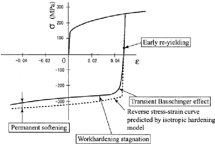
two items relate specifically to multiaxial cycling. Some of these phenomena are shown in Figure 2.4. for the uniaxial state, since the vast majority of the experiments and modelling have been applied to uniaxial cycling.

Figure 2.4. An example of stress-strain response in a forward-reverse deformation in uniaxial state (Yoshida and Uemori, 2003).

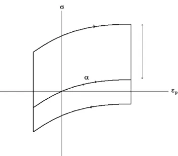
A common feature of all of the models considered is their use of a “backstress” to account for the stress space symmetry. The differences arise from the way the backstress develops. These models can be characterized by evolution laws for the backstress and can be evaluated in terms of how well they can represent the conditions described above. When considering these cyclic plasticity models, attention is given to the backstress evolution, or kinematic portion. In some applications no isotropic hardening is used (Mroz models) but for most of these models a monotonic increase in the yield surface radius is allowed (as explained in the previous subsection). A brief summary of the models listed above is given in the following. The highlights of their suitability to model the above mentioned phenomena are also considered.

2.4.2.1. Prager-Ziegler linear kinematic model