Feedback EDF Scheduling Exploiting
Hardware-Assisted Asynchronous Dynamic Voltage Scaling
∗Yifan Zhu and Frank Mueller
Department of Computer Science/Center for Embedded Systems Research
North Carolina State University,Raleigh, NC 27695-7534
[email protected], phone: +1.919.515.7889, fax: +1.919.515.7925
Abstract
Power consumption has been a major concern, both for processor design with high clock rates and embed-ded systems driven by batteries. Recent support for dy-namic frequency and voltage scaling (DVS) in contem-porary processor architectures allows software to affect power consumption by varying execution frequency and supply voltage on the fly. However, processors generally enter a sleep state while transitioning between frequen-cies/voltages. In this paper, we examine the merits of hardware/software co-design for a feedback DVS algo-rithm and a novel processor capable executing instruc-tions during frequency/voltage transiinstruc-tions. We study several power-aware feedback schemes based on earliest-deadline-first (EDF) scheduling that adjust the system behavior dynamically for different workload characteris-tics. An infrastructure for investigating several hard real-time DVS schemes, including our feedback DVS algo-rithm, is implemented on an IBM PowerPC 405LP em-bedded board. Architecture and algorithm overhead is as-sessed for different DVS schemes. Measurements on an experimentation board provide a quantitative assessment of the potential of energy savings for DVS algorithms as opposed to our prior simulation work that could only provide trends. Energy consumption, measured through a data acquisition board, indicates a considerable pottial for real-time DVS scheduling algorithms to lower en-ergy up to 64% over the na¨ıve DVS scheme. Our feed-back DVS algorithm at least as much and often consid-erably more energy than previous DVS algorithms with peak savings of an additional 24% energy reduction.
1. Introduction
Energy consumption has become a vital design con-straint in embedded systems for a long time. The de-mand for efficient energy management is increasing in hand-held and embedded devices, where battery ser-vice life is usually critical to system performance. For
∗ This work was supported in part by NSF grants CCR-0208581, CCR-0310860 and CCR-0312695.
many non-battery powered systems, energy consump-tion is also an important cost factor due to environ-ment issues. The processor is one of the most power-consuming devices of a computer. In order to reduce the CPU energy consumption, Dynamic Voltage Scal-ing (DVS) technology has been widely supported in re-cent years for extending battery life. DVS dynamically scales the processor core voltage up or down depending on the computational demand of the system. Reducing the supply voltage results in a lower transistor switch-ing speed, which also allows a lower clock frequency. Assuming that voltage and frequency are linearly re-lated, scaling down both voltage and frequency results in cubic reduction of power consumption (P ∝V2
×f) [5]. While useful for simulation, this formula cannot re-flect architectural details that this study focuses on.
DVS algorithms have been intensively studied for both non real-time and real-time systems [21, 1, 14, 7, 9, 20, 24]. In the case of retime systems, the DVS al-gorithm calculates a safe frequency that provides just enough processing resources to finish a given task be-fore its deadline. The goal is to save the maximum pos-sible amount of energy and still guarantee the schedu-lability of hard real-time systems where all tasks are required to meet their deadlines.
We examine all these issues by integrating our feed-back DVS algorithm within a real-time EDF sched-uler. An infrastructure to assess our algorithm as well as several other DVS algorithms is implemented on an IBM PowerPC 405LP embedded board, which was specially modified for power management research. A unique DVS feature supported by the test board is that frequency switching can be done either synchronously or asynchronously, both of which we evaluated exper-imentally for different DVS algorithms. We show the strength of our feedback DVS algorithm by compar-ing the actual energy consumption with other DVS al-gorithms.
The rest of this paper is organized as follows. Sec-tion 2 gives a brief introducSec-tion of the DVS schedul-ing framework and task model. Section 3 discusses our DVS algorithm and two feedback mechanisms proposed for the practical environment. Detailed experimental results are presented in Section 4. Section 5 discusses some of the related work. Conclusions are given in Sec-tion 6.
2.
EDF Scheduling with DVS Support
In order to assess DVS algorithms for their suit-ability and energy saving performance in an embed-ded environment, we consider the scheduling problem in hard real-time systems with the earliest deadline first (EDF) policy. The entire scheduler framework consists of two components: (1) an EDF scheduler and (2) a DVS scheduler. These two components are indepen-dent of each other so that the EDF scheduler is ca-pable of working with different DVS algorithms. EDF is especially attractive to DVS algorithms because of its dynamic property, which allows the DVS scheduler to exploit slack. Our DVS scheduler is based on feed-back control that incrementally adjusts system behav-ior in order to reduce energy consumption.
A periodic, fully preemptive and independent task model is used in the framework. Each taskTiis defined
by a triple (Pi, Ci, ci), wherePi is the period ofTi,Ci
is the measured worst-case execution time of Ti, and
ci is the actual execution time of Ti. Each task’s
rel-ative deadline, di, is equal to its period, and all tasks
are released at time zero. The periodically released in-stances of a task are called jobs.Tij is used to denote
the jth job of taskT
i. Its release time is Pi∗(j −1)
and its deadline isPi∗j.cijis used to represent the
ac-tual execution time of job Tij. The hyperperiod H of
the task set is defined as the least common multiplier (LCM) among all the tasks’ periods. The schedule re-peats at the end of each hyperperiod.
In the following, we describe in detail the feedback DVS scheduler and several feedback schemes used in the framework.
3. Feedback DVS Algorithm
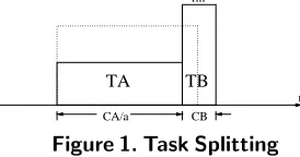
Our feedback DVS algorithm anticipates an actual execution time of each task invocation (a job) based on the feedback from the execution time in previous invocations. It then splits the execution budget of a task into two parts, as depicted in Figure 1. The an-ticipated actual time CA is scaled at the lowest
pos-sible frequency. Conversely, the remaining execution timeCB is scaled at the maximum frequency such that
CA+CB=W CET.
TB TA
CA/a CB
t fm
Figure 1. Task Splitting
All future tasks are deferred as long as possible us-ing a maximal (worst-case) schedule, which is related to the actual schedule to derive the currently available slacksk for taskk. Thus,
α= CA
CA+sk
indicates the scaling factor and the corresponding low-est possible frequency. The algorithm is capable of cap-turing changes in actual execution times using a feed-back scheme. Preemption of the current task is antic-ipated via future slot allocations in the schedule. It is implemented in a backward sweep to fill idle and early completion slots from a task’s deadline back-wards (for algorithmic details, see [25]). Due to the even more greedy approach than any of the previous schemes, the algorithm was reported to exhibit addi-tional energy savings in simulation experiments, par-ticularly for medium utilization systems, which are quite common [6]. Even more substantial savings have been observed for fluctuating execution times where PID-feedback provides new opportunities for aggres-sive scaling [25]. During the implementation of the al-gorithm for the 405LP embedded board, we refined the feedback scheme proposed in [25] and developed the fol-lowing two feedback mechanisms.
3.1. Simple Feedback
such as the PID-feedback controller described in the next section, because a simple feedback usually pro-vides good enough performance in this case. The quan-titative comparison of the overhead between our PID-feedback DVS algorithm and several other DVS algo-rithms (detailed in Section 4) also makes us believe that a complicated feedback DVS scheme degrades its energy saving potential to some extend.
The simple feedback mechanism chooses the value of
CAas the controlled variable. Each jobTij’s actual
ex-ecution time cij is chosen as the set point. CA is
as-signed to be 50% WCET for the first job of each task, which means half of the job’s execution is budgeted at a low frequency, and half of it is reserved at the maxi-mum frequency. The maximaxi-mum frequency portion guar-antees the deadline requirements, even if the worst-case execution time is used in full. Each time a job com-pletes, its actual execution time is fed back and aggre-gated to anticipate the next job’sCA. LetCAij denote
theCAvalue forTij. The (j+ 1)thjob of the task is
as-signed aCA value according to:
CAi(j+1)= (CAij+ci(j+1)−ci(j−N+1))/N (1)
where N is a constant representing the number of items used in the moving average calculation. Our ex-periments show significant energy savings for such a simple feedback mechanism with very low scheduling overhead as long as the workload’s actual execution time exhibits a stable behavior during some interval. When the workload’s behavior keeps changing dynam-ically with highly fluctuating execution times, simple feedback becomes not enough to yield the best energy savings. In those cases, a more sophisticated feedback mechanism is required, as detailed in the next section.
3.2. PID Feedback
The original PID-feedback DVS mechanism, as pre-sented in [25], requires the DVS scheduler to cre-ate and maintain multiple independent feedback con-trollers for each of the tasks in the workload. Multi-ple inputs and multiMulti-ple outputs need to be manip-ulated simultaneously by the DVS scheduler. Such a PID-feedback mechanism, albeit its potential for en-ergy savings shown in our previous simulation exper-iments, results in substantial execution overhead on an embedded architecture. Giving the difficulty of pre-cisely characterizing the behavior of a multiple-input multiple-output control system, it also adds complex-ity to the theoretical analysis of the algorithm. There-fore, we refine the original PID-feedback DVS mecha-nism by the following simplified design.
Instead of usingCAi(i= 1...n) as the controlled
vari-able for each task Tiand creatingndifferent feedback
controller for n different tasks, we now define a
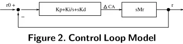
sin-+ −
r0 r
sMr Kp+Ki/s+sKd CA
Figure 2. Control Loop Model
gle variable r as the controlled variable for the entire system as:
r= 1
n
n
X
i=1
CAij−cij
cij
(2)
where j is the index of the latest job of task Ti
be-fore the sampling point. Our objective is to maker ap-proximate 0 (i.e.,the set point). The system error be-comes
(t) =r−0. (3)
(t) is fed back to the PID scheduler to regulate the controlled variable r. The PID feedback controller is now defined as:
∆rj =Kpi(t) +K1i P
IWi(t) +Kd
i(t)−i(t−DW)
DW
rj+1 =rj+ ∆rj
(4) For each rj, we adjust the CA value for taskTi by
CAi(j+1) = rjcij +cij. The transfer function Gr
be-tween randCAcan be derived by taking derivative of
both sides of the equation 2:
Gr(s) =Mrs (5)
where Mr = n1Pni=1c1i. The block diagram of the
model is shown in Fig. 2. Its transfer function is :
GP(s)Gr(s)
1 +GP(s)Gr(s)
= M Kps+M Ki+M Kds
2
1 +M Kps+M Ki+M Kds2
(6)
According to control theory, a system is stable if and only if all the poles of its transfer function are in the negative half-plane of the s-domain. From Equa-tion 6, we infer the poles of our system as
−M Kp±√M Kp2−4M Kd(M Ki+ 1)
2M Kd
(7)
Note that −M Kp+√M Kp2−4M Kd(M Ki+ 1) is
still less than 0 when M K2
p −4M Kd(M Ki+ 1) >0.
Hence, all the poles are in the negative half-plan of the s-domain. Therefore, the stability of the above system is ensured.
Such a single controller mechanism is easy to imple-ment because just one feedback controller suffices for the entire system, which reduces the complexity and overhead of the feedback DVS algorithm. But it also has its drawback,i.e., it does not provide direct feed-back information of the CA value for each individual
It is an imprecise description of the original scheduling objective and may take longer to get the system into a stable status. Nonetheless, our experiment shows sig-nificant energy savings of this feedback DVS mecha-nism with much reduced overhead compared to other DVS algorithms. In the next section, we present the de-tails of our experimental results.
4. Experimental Evaluation
By evaluating our feedback DVS algorithm on a real embedded architecture, we assess the true po-tential of our algorithm for energy savings in an ac-tual system as opposed to a simulation environment. Also, we compare the overhead and energy consump-tion between our algorithm and several other DVS al-gorithms, namely static DVS, cycle-conserving DVS, look-ahead-1/2 DVS (all by Pillai and Shin [21]) as well as DR-OTE and AGR-2 (by Aydin et al. [1]). Look-ahead-1 and look-ahead-2 are the original and a modified version of the original look-ahead DVS algo-rithm in [21], respectively. Look-ahead-1 updates each task’s absolute deadline immediately when a task in-stance completes. Look-ahead-2 delays such update till the next task instance is released, which results in addi-tional energy savings. AGR-2 follows the most aggres-sive scheme presented in [1] with an aggresaggres-siveness pa-rameter k of 0.9. In these experiments, we also wanted to determine if the lower frequencies and voltages cho-sen by our feedback scheme outweigh the higher com-putational overhead required to make scheduling deci-sions.
4.1. Platform and Methodology
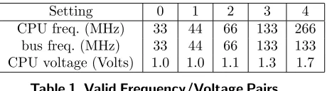
The embedded platform used in our experiment is a PowerPC 495LP embedded board running on a diskless MontaVista Embedded Linux variant, which is based on the 2.4.21 stock kernel but has been patched to sup-port DVS on the PPC 405LP. This board provides the hardware support required for DVS and allows soft-ware to scale voltage and frequency via user-defined operation points ranging from a high end of 266 MHz at 1.8V to a low end of 33 MHz at 1V [19, 4, 10]. The board has also been modified for 50% reduced ca-pacitance, which allows DVS switches to occur more rapidly, i.e., switches are bounded by at most a 200 microseconds duration from 1V to 1.8V. The DVS al-gorithms (static, cycle-conserving, look-ahead [21] and our feedback DVS) were exposed to the DVS capabil-ities of the 405LP board. The scheduling algorithms can choose any frequency/voltage pair from the set de-picted in Table 1.
This set of pairs was constrained by a need to have a common PLL multiplier of 16 relative to the 33MHz base clock and a divider of two or any multiple of 4. Changing the multiplier incurs additional overhead for
Setting 0 1 2 3 4
CPU freq. (MHz) 33 44 66 133 266 bus freq. (MHz) 33 44 66 133 133 CPU voltage (Volts) 1.0 1.0 1.1 1.3 1.7
Table 1. Valid Frequency/Voltage Pairs
switching, which we wanted to eliminate in this study. A dynamic power management (DPM) facility [4] is de-veloped as an enhancement to the Linux kernel to sup-port DVS features. DPMoperating pointdefines stable frequency/voltage pairs (as well as related system pa-rameters), which we experimentally determined.
In order to assess power consumption, we need to monitor processor core voltage and current at a high rate. Hence, we used a high-frequency analog data ac-quisition board to gather data for (a) the processor core voltage and (b) the processor current. The lat-ter was measured as a voltage level over a resistor with a 1V drop per 360mA. Power consumption was com-puted by multiplying the CPU voltage with its current. Data acquisition board allowed us to experiment with longer-running applications to assess the energy con-sumption of the processor, which is the integration of power over time. We also employed an oscilloscope for visualizing the voltages and currents with high preci-sion in readings.
We implemented an EDF scheduler as a user-level thread library under Linux on the 405LP board. A user-level library was chosen over a kernel-user-level solution be-cause of the simplicity of its design and the fact that the operating system background activity is minimal on the embedded board infrastructure. Different DVS scheduling schemes were attached into the EDF sched-uler as independent modules.
4.2. Synchronous vs. Asynchronous Switch
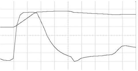
We first assessed the overhead of different DVS tech-niques supported by the test board and the dynamic power management extensions of the operating system. A unique DVS feature supported by the IBM PPC 405LP embedded board is that frequency switching can be done either synchronously or asynchronously. Synchronous switching is the traditional approach for processor frequency/voltage transitions, where appli-cations have to stop execution during the transi-tional interval. Asynchronous switching, on the con-trary, allows application to continue execution during the frequency/voltage transitions. Figure 3 depicts the changes in current (lower curve) and voltage (upper curve) of the PPC 405LP processor core during an asynchronous switch.Figure 3. Current and Voltage Transition During Asynchronous Frequency Switching
to ramp up towards the maximum as fast as possible (the 30 degree voltage ramp on the upper curve of Fig-ure 3). Meanwhile, the time to reach a voltage level at least as high as required by the new frequency is esti-mated. A high-resolution timer is programmed to inter-rupt when this duration expires, prior to which the ap-plication can still continue execution. Once the timer interrupt triggers its handler (at the peak after the 30 degree ramp on the upper curve), the power manage-ment unit is reprogrammed to settle at the target volt-age level, and the new processor frequency is activated before returning from the handler. The voltage then settles (in case it overshot) in a controlled manner to the new operating point. The current also settles in a controlled manner depending on the actual process-ing activity.
Table 2 reports the overhead for synchronous and asynchronous switching in a time range bounded by two extremes: (a) Switching between adjacent fre-quency/voltage levels and (b) switching between the lowest and highest frequency/voltage levels. Further-more, the overhead of the subsequent signal handler associated with each asynchronous switch is also mea-sured for a range of the highest and the lowest proces-sor frequencies. The results indicate that a synchronous DVS switch has about an order of a magnitude larger overhead than an asynchronous switch. The timer in-terrupt handler triggered at each asynchronous switch only increases the overall overhead insignificantly.
activity sync. DVS async. DVS signal handler overhead 117-162µsec 8-20µsec 0.07-0.6µsec
Table 2. DVS Switching Overhead
4.3. DVS Scheduler Overhead
We compared the overhead of our feedback-DVS al-gorithm with several other dynamic DVS alal-gorithms. We first measured the execution time of these DVS
scheduling algorithms under different frequencies on the embedded board, as depicted in Table 3. The over-head was obtained by measuring the amount of time when a task issues a yield() system call till another task was dispatched by the scheduler. The table shows that static DVS has the lowest overhead among the four while our PID-feedback DVS has the highest one. This is not surprising since static DVS uses a very sim-ple strategy to select the frequency and voltage falling short in finding the best energy saving opportunities. Cycle-conserving DVS, look-ahead DVS and our PID-feedback DVS use more sophisticated and aggressive al-gorithms for lower energy consumption, albeit at higher overheads. The trade-off between overhead and perfor-mance always needs to be examined carefully.
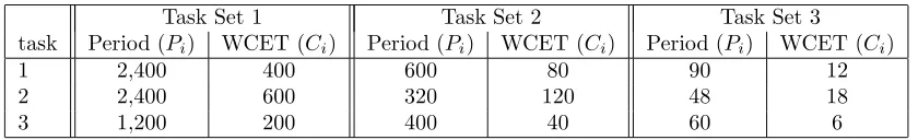
Next, we assessed if our feedback-DVS algorithm, al-though incurring the largest overhead among the four, gives the best energy saving results in the real em-bedded environment. We measured the actual energy consumption of these DVS algorithms when executing three medium utilization task sets depicted in Table 4 using both synchronous and asynchronous DVS switch-ings. As a baseline for comparison, we also implemented a na¨ıve DVS scheme where the maximum frequency is always chosen whenever a task is scheduled, and the minimum frequency is always chosen whenever the sys-tem is idle.
DVS scheduling overhead[µsec]
CPU freq. static cc look-ahead PID-feedback
33 MHz 217 487 2296 3612
44 MHz 170 366 1714 2943
66 MHz 100 232 1112 1728
133 MHz 52 120 546 801
266 MHz 36 76 229 472
Table 3. Overhead of DVS-EDF Scheduler
The first task set in Table 4 is harmonic,i.e., all pe-riods are integer multiples of the smallest period, which facilitates scheduling. This often allows scheduling al-gorithms to exhibit an extreme behavior, typically out-performing any other choice of periods. The second and third task sets are non-harmonic with longer and shorter periods, respectively. Actual execution times were half that of the WCET for each task for this ex-periment.
Task Set 1 Task Set 2 Task Set 3
task Period (Pi) WCET (Ci) Period (Pi) WCET (Ci) Period (Pi) WCET (Ci)
1 2,400 400 600 80 90 12
2 2,400 600 320 120 48 18
3 1,200 200 400 40 60 6
Table 4. Task Set, times in msec
algorithm na¨ıve static static save cycle-cons. c-c save look-ahead l-a save our feedback fdbk save Task Set 1
sync. 4.47 3.2 28.41% 2.38 46.61% 2.21 50.56% 2.04 54.21% async. 4.43 3.13 29.35% 2.327 47.51% 2.12 52.07% 2.00 54.70%
savings 0.89% 2.19% 2.51% 3.92% 1.95%
Task Set 2
sync. 0.544 0.5056 7.06% 0.4713 13.36% 0.424 22.06% 0.4089 24.83% async. 0.5276 0.5025 4.76% 0.4622 12.40% 0.4218 20.05% 0.4064 22.97%
savings 3.01% 0.61% 1.93% 0.52% 0.61%
Task Set 3
sync. 0.595 0.5616 5.61% 0.4799 19.34% 0.4043 32.05% 0.3708 37.68% async. 0.5802 0.5496 5.27% 0.4547 21.63% 0.3912 32.57% 0.3671 36.73%
savings 2.49% 2.14% 5.25% 3.24% 1.00%
Task Set 2 vs. Task Set 3
change 9.07% 8.57% -1.65% -7.82% -10.71%
Table 5. Energy [mW −hrs] consumption per RT-DVS algorithm
clearly shows the tremendous potential in energy sav-ings for real-time scheduling.
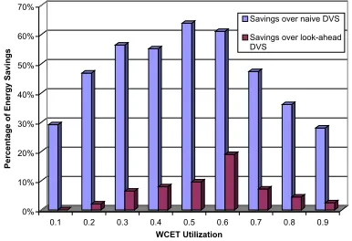
The savings for each algorithm are lower for task set two peaking at about 23% for our feedback scheme. As mentioned before, task set one is harmonic, which typi-cally results in the best scheduling (and energy) results since execution is more predictable. Task set three lies in between the other two with peak savings of 37% for our feedback scheme.
The results also demonstrate that the overhead for calculations inherent to scheduling algorithms is out-weighed by the potential for energy savings. This is un-derlined by the increasing overhead in execution time for each of the scheduling algorithms (from left to right in Table 5) accompanied by decreasing energy con-sumption.
Another noteworthy result is the comparison be-tween synchronous and asynchronous DVS switching depicted in the last row for each task set in Table 5. For each of the scheduling algorithms, we see addi-tional savings of 1-5% on asynchronous switching due to the ability to commence with a task’s execution dur-ing frequency and voltage transitions. We also ran ex-periments with task sets that had an order of a magni-tude smaller periods and execution times. Surprisingly, the synchronousvs.asynchronous savings remained ap-proximately the same, even though DVS switches oc-cur ten times as often. We believe that the periods and
execution time settings used in our experimental envi-ronment are still large compared to the execution time of a synchronous or asynchronous switching. If we only save about 100 µsec at each frequency switch (as has been shown in Table 2) but later on spend more then 10-100 msec in running a task, the benefit of the asyn-chronous DVS switching becomes insignificant. These results seem to indicate that the benefit of continuous execution during DVS switching, although not negligi-ble, is secondary to trying to minimize the overhead of DVS scheduling itself.
We also compared task sets two and three in terms of their absolute energy readings, which is valid since they executed for the same amount of time (ten seconds), the same actual to worst-case execution time ration and the same utilization, albeit at seven times more context switches. This change is depicted in the last row of Table 5 for the asynchronous case. Not surpris-ingly, the energy with na¨ıve DVS is about 9% higher for task set three than for set two due to the higher context switch overhead of the latter. Quite interest-ingly, this overhead turns into a reduction in energy as DVS schemes become more aggressive.
4.4. Impact of Different Workloads
indepen-dent periodic tasks whose worst-case execution time varies from 0.1 to 0.9 with an increment of 0.1. The ac-tual execution time of a task is determined by tim-ing the body of each task plus the scheduler over-head (see Table 3) of the corresponding DVS algo-rithm under the lowest CPU frequency. We dynam-ically changed the number of instructions inside each task body among different invocations,i.e., jobs, to ap-proximate the workload fluctuation behavior of actual real-time applications.
Altogether, four synthesized execution patterns were created. For the first pattern, a task’s actual execution time is always 50% WCET. For the second pattern, the actual execution time of a task drops exponentially be-tween a peak value and 50%WCET among its consec-utive jobs, modeled asci= 1/2(t−cm). The peak value
cm was chosen to be 20%WCET. This pattern
sim-ulates event-triggered activities that result in sudden, yet short-term computational demands due to complex inputs often observed in interrupt-driven systems. The third pattern is similar to the second one except that it drops more gradually, modeled asci=cmsin(t+π/2).
This pattern simulates events resulting in computa-tional demands in a phase of subsequent complex in-puts with a decaying tendency. For the fourth pat-tern, the actual execution time of a task increases and decreases gradually around 50% WCET, modeled as
ci=cmsin(t) andci=−cmsin(t). This pattern
repre-sents periodically fluctuating activities with gradually increasing and decreasing computational needs around peaks. We used simple feedback on pattern 1 because of its nearly constant execution time pattern among different jobs. The number of items to compute the moving average was set asN = 10. PID-feedback was used on patterns 2, 3, and 4 to exploit fluctuating exe-cution time characteristics. The PID parameters were chosen by tuning manually withKp = 0.9,Ki = 0.08,
Kd= 0.1. The derivative and integral window size were
1 and 10, respectively. Asynchronous switching was al-ways used in this experiment since it has a better per-formance than synchronous switching.
Figure 4 and Figure 5 present the energy consump-tion of our feedback-DVS as well as four other dy-namic DVS algorithms under task execution pattern 2. The number of tasks in the task set varies between 3 and 30 tasks. All energy values are normalized to the na¨ıve DVS results. AGR-2 dynamically reclaims un-used slack up to the next arrival time of any task in-stance (NTA), hence saving about 50% extra energy than na¨ıve DVS. AGR-2 is not as good as Look-ahead-1/2 DVS for 3 tasks since it considers slack only up to the next task instance’s deadline, while Look-ahead DVS collects slack up to the largest deadline among
Figure 4. PID feedback for 3-task sets with dy-namic exec. time pattern 2
Figure 5. PID feedback for 30-task sets with dy-namic exec. time pattern 2
all tasks. But AGR-2 benefits from smaller task gran-ularity in 30-task sets and outperforms Look-ahead-1 for extreme utilizations (small and large) except for the range of 0.5-0.7 utilization. When compared with Look-ahead-2, AGR only outperforms it for hight uti-lizations, otherwise Look-ahead-2 performs better.
Our feedback-DVS shows additional benefits over both Look-ahead-2 AGR-2. Relative to the two schemes, we save another 5%-20% energy due to our algorithm’s self-adaptation to jobs’ actual execution times. In cases of extremely low utilization,
Figure 7. PID feedback for task sets with dynamic exec. time pattern 2
Figure 8. PID feedback for task sets with dynamic exec. time pattern 3
DVS, Look-ahead DVS and AGR-2 are observed to re-sult in virtually the same energy savings because every task has enough slack to run at the minimum speed re-sulting in the same frequencies for a schedule irrespec-tive of the DVS algorithm.
Let us now focus on the comparison of our algo-rithm with the look-ahead-2 DVS algoalgo-rithm for 3-task sets, but under different dynamic execution time pat-terns. Figure 6 shows that when each task has a nearly
Figure 9. PID feedback for task sets with dynamic exec. time pattern 4
Figure 10. Pattern 4 with Different Avg. Exec. Times – Energy Normalized to Na¨ıve DVS
constant execution time among different instances, our simple feedback DVS saves up to 19% more energy than look-ahead-2 DVS. We notice a reduction in energy sav-ings when utilization becomes extremely low or high. Such extreme utilizations force all tasks to run at the minimum or the maximum frequency. On average, the simple feedback DVS outperforms look-ahead by 10% and outperforms na¨ıve DVS by about 50%.
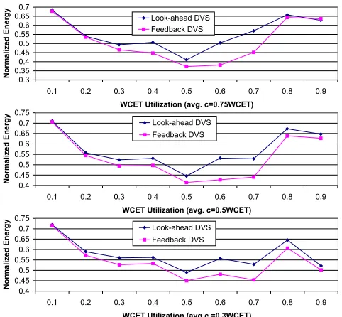
Figures 7-9 shows the energy consumption with dy-namic execution time patterns 2, 3 and 4. The maximal savings over look-ahead-2 are 11%, 15% and 20%, re-spectively. The maximal savings over na¨ıve DVS are be-tween 25% and 60%. The largest savings again happen in median utilization cases where there is considerable dynamic slack. PID-feedback mechanism helps capture the dynamic behavior of task execution times and to subsequently scale power even more aggressively than other DVS algorithms. Although look-ahead DVS can also take advantage of dynamic slack and lower the fre-quency/voltages more aggressively than na¨ıve DVS, it lacks a feedback scheme to adjust its behavior dynam-ically. From time to time, it has to overcome the fact that the frequency was lowered too much in the past by raising the voltage and frequency to a level even higher than the safe frequency.
can scale equally well for loose and tight execution-time patterns. In all three cases, 14% to 24% addi-tional energy is saved than for look-ahead DVS. Our PID-feedback mechanism shows even better strength for median and tight execution time cases than the loose execution time case because capturing the dy-namic behavior of a task’s actual execution time in a tight execution environment is more critical than in a loose environment.
Figure 11 depicts screen-shots of voltage and current obtained from the oscilloscope for the phase just after a simultaneous release of all tasks at the beginning of a hyperperiod. Static DVS shows two levels of voltages (busy/idle time) whereas cycle-conserving DVS
differ-2V
1V t
0mA 360mA
(a) static RT-DVS EDF
2V
1V t
0mA 360mA
(b) cycle-conserving RT-DVS EDF
2V
1V t
0mA 360mA
(c) look-ahead RT-DVS EDF
2V
1V t
0mA 360mA
(d) our feedback RT-DVS EDF
Figure 11. Voltage/current oscilloscope
shot with loose WCET: W CET =
2×ActualExecT ime, U tilization U= 0.5
entiates three levels on a dynamic base. Even lower voltage and current readings are given by look-ahead DVS, which not only distinguishes more levels but also exhibits much lower power levels during load. The low-est results were obtained by our feedback DVS, which defers execution even more aggressively than any of the other methods. However, our feedback scheme can only further reduce power consumption occasionally as suf-ficient slack exists to be recovered by the algorithms of the previous schemes. Dynamic slack is recovered in in-creasing levels by the latter three schemes.
4.5. Comparison with Simulation Results
When we compare the energy saving results ob-tained from the IBM 405LP embedded board with our previous simulation results presented in [25], we clearly see the advantage and disadvantage of tion for power-aware studies. The advantage of simula-tion lies in its ease of implementasimula-tion and predictabil-ity of performance trends. The energy consumption of different DVS algorithms show a consistent trend un-der both simulation and the actual embedded platform. But quantitative results differ. Our previous simulation results reported 5%-10% higher savings on average. For example, the best energy saving of our feedback DVS over look-ahead DVS was report as 29% in simulation while the best result we measured from the test board is around 24%. It is also non-trivial to model the actual power/energy consumption in simulation without con-sidering actual hardware details. This is also the case when evaluating the overhead. Since the overhead of DVS algorithms was not included in our previous sim-ulation experiment, we still observed 7%-10% energy savings over look-ahead DVS even at high utilization cases. But the actual energy measurement from the test board show only 3%-6% savings for these cases.Overall, our experiments on the embedded platform quantitatively show the potential of our feedback DVS algorithm and its ability to scale power even more ag-gressively than previous DVS algorithms.
5. Related Work
in-cluding both periodic and aperiodic tasks, are further investigated by Aydin and Yang in [3]. Gruian analyzes a dual-speed DVS schedule based on stochastic data de-rived from past task execution traces [8]. Jejurikar and Gupta investigate static and dynamic slowdown fac-tors for periodic tasks [12] and combine it with pro-crastination scheduling [13] and preemption threshold scheduling [11] for DVS.
The potential of feedback control on real-time scheduling was first investigated by Stankovic et al. [22]. Real-time system performance specifications are analyzed systematically through a control-theoretical methodology by Luet al.[15]. A feedback-control real-time scheduling framework for unpredictable dynamic real-time systems is further proposed by Luet al.where task execution times diverge from their worst case [16]. Dynamic models of real-time systems are developed to identify different categories of real-time applications with different feedback control algorithms.
Feedback control was also proposed for energy-aware computing in previous work, such as those by Varma [23], Lu [17] and Minerick [18]. Varma et al. present a feedback-control algorithm where the previous work-load execution history is used to predict the future workload behavior by a discrete-time PID function. The combination of the proportional, integral and derivative part of the PID function provides good es-timation across different applications insensitive of the change of their parameters [23]. Lu et al. describe a formal feedback-control algorithm combined with dy-namic voltage/frequency scaling technologies. While Varma and Lu’s work targets soft real-time/multimedia systems, our feedback DVS scheme focuses on hard real-time system where timing constraints must not be violated. A general energy management scheme with feedback control is proposed by Minericket al.[18]. Av-erage energy usage is achieved by continuously adjust-ing the voltage/frequency of a processor to meet the energy consumption goal. The objective of their work is to obtain low energy consumption for general pur-pose systems while our work targets hard real-time sys-tems with deadline requirements.
6. Conclusion
In this paper, we presented feedback DVS algorithm considering practical design and implementation issues. We evaluated it as well as several other real-time DVS algorithms on an IBM 405LP embedded platform. An unique DVS feature of this platform is asynchronous frequency switching, which supports continued exe-cution during voltage/frequency transitions. We have shown up to 5% energy savings of asynchronous switch-ing for fast DVS modulation without enterswitch-ing sleep modes as opposed to traditional synchronous
switch-ing. We assessed the benefits of our feedback DVS al-gorithm by measuring the energy consumption over the hyperperiod of real-time tasks. Energy consump-tion as well as scheduling overhead between different DVS schemes were compared with each other. The ex-perimental results indicate that our aggressive feedback DVS scheduling algorithm achieves up to 24% addi-tional savings in energy consumption over the look-ahead DVS and AGR-2 algorithms and up to 64% en-ergy savings over the na¨ıve DVS scheme when consid-ering scheduling overheads.
Acknowledgments
Ajay Dudani contributed to early work of the Feedback-DVS scheme [6]. Aravindh V. Anantara-man, Ali El-Haj Mahmoud, Ravi K. Venkatesan de-signed and implemented an early version of the DVS experimentation environment. Bishop Brock from IBM provided most valuable technical details for the PPC 405LP board, which was donated by IBM Re-search (Austin). This work was supported in part by NSF grants 0208581, 0310860 and CCR-0312695.
References
[1] H. Aydin, R. Melhem, D. Mosse, and P. Mejia-Alvarez. Dynamic and agressive scheduling techniques for power-aware real-time systems. InIEEE Real-Time Systems Symposium, Dec. 2001.
[2] H. Aydin, R. Melhem, D. Mosse, and P. Mejia-Alvarez. Power-aware scheduling for periodic real-time tasks. IEEE Trans. Comput., 53(5):584–600, 2004.
[3] H. Aydin and Q. Yang. Energy-responsiveness tradeoffs for real-time systems with mixed workload. In Proceed-ings of the 11th IEEE Real-Time and Embedded Tech-nology and Applications Symposium, May 2004. [4] B. Brock and K. Rajamani. Dynamic power
manage-ment for embedded systems. InIEEE International SOC Conference, Sept. 2003.
[5] A. Chandrakasan, S. Sheng, and R. W. Brodersen. Low-power cmos digital design. InIEEE Journal of Solid-State Circuits, Vol. 27, pp. 473-484., April, 1992. [6] A. Dudani, F. Mueller, and Y. Zhu. Energy-conserving
feedback edf scheduling for embedded systems with real-time constraints. InACM SIGPLAN Joint Conference Languages, Compilers, and Tools for Embedded Systems (LCTES’02) and Software and Compilers for Embedded Systems (SCOPES’02), pages 213–222, June 2002. [7] K. Govil, E. Chan, and H. Wasserman. Comparing
algo-rithms for dynamic speed-setting of a low-power cpu. In 1st Int’l Conference on Mobile Computing and Network-ing, Nov 1995.
[9] D. Grunwald, P. Levis, C. M. III, M. Neufeld, and K. Farkas. Policies for dynamic clock scheduling. In Symp. on Operating Systems Design and Implementa-tion, Oct 2000.
[10] IBM and M. Software. Dynamic power management for embedded systems. white paper.
[11] R. Jejurikar and R. Gupta. Integrating preemption threshold scheduling and dynamic voltage scaling for en-ergy efficient real-time systems. InProceedings of the 10th International Conference on Real-Time and Em-bedded Computing Systems and Applications (RTCSA ’04), 25-27 Aug 2004.
[12] R. Jejurikar and R. Gupta. Optimized slowdown in real-time task systems. InProceedings of the 16th Euromi-cro Conference on Real-Time Systems (ECRTS ’04 ), Jun30-Jul2 2004.
[13] R. Jejurikar and R. Gupta. Procrastination scheduling in fixed priority real-time systems. InProceedings of the Language Compilers and Tools for Embedded Systems, Jun 2004.
[14] D. Kang, S. Crago, and J. Suh. A fast resource synthe-sis technique for energy-efficient real-time systems. In IEEE Real-Time Systems Symposium, Dec. 2002. [15] C. Lu, J. A. Stankovic, T. F. Abdelzaher, G. Tao, S. H.
Son, and M. Marley. Performance specifications and metrics for adaptive real-time systems. InProceedings of the IEEE Real-Time Systems Symposium, December 2000. 2000.
[16] C. Lu, J. A. Stankovic, G. Tao, and S. H. Son. Feedback control real-time scheduling: Framework, modeling, and algorithms.Real-Time Syst., 23:85–126, 2002.
[17] Z. Lu, J. Hein, M. Humphrey, M. Stan, J. Lach, and K. Skadron. Control-theoretic dynamic frequency and voltage scaling for multimedia workloads. In Interna-tional Conference on Compilers, Architectures, and Syn-thesis for Embedded Systems, pages 156–63, 2002. [18] R. Minerick, V. W. Freeh, and P. M. Kogge. Dynamic
power management using feedback. InProceedings of Workshop on Compilers and Operating Systems for Low Power, 2002.
[19] K. Nowka, G. Carpenter, and B. Brock. The design and application of the powerpc 405lp energy-efficient system on chip. IBM Journal of Research and Development, 47(5/6), September/November 2003.
[20] T. Pering, T. Burd, and R. Brodersen. The simulation of dynamic voltage scaling algorithms. InSymp. on Low Power Electronics, 1995.
[21] P. Pillai and K. Shin. Real-time dynamic voltage scal-ing for low-power embedded operatscal-ing systems. In Sym-posium on Operating Systems Principles, 2001.
[22] J. A. Stankovic, C. Lu, S. H. Son, and G. Tao. The case for feedback control real-time scheduling. InProceedings of the EuroMicro Conference on Real-Time Systems, June 1999.
[23] A. Varma, B. Ganesh, M. Sen, S. R. Choudhury, L. Srini-vasan, and J. Bruce. A control-theoretic approach to dy-namic voltage scheduling. InProceedings of the 2003 in-ternational conference on Compilers, architectures and
synthesis for embedded systems, pages 255–266. ACM Press, 2003.