Performance of Buckets versus Min-Heap in the A* Search Algorithm

(1)

Scholarship at UWindsor

Electronic Theses and Dissertations Theses, Dissertations, and Major Papers

9-17-2019

Performance of Buckets versus Min-Heap in the A* Search

Algorithm

Sheeba Mohanraj

University of Windsor

Follow this and additional works at: https://scholar.uwindsor.ca/etd

Recommended Citation Recommended Citation

Mohanraj, Sheeba, "Performance of Buckets versus Min-Heap in the A* Search Algorithm" (2019). Electronic Theses and Dissertations. 7823.

https://scholar.uwindsor.ca/etd/7823

This online database contains the full-text of PhD dissertations and Masters’ theses of University of Windsor students from 1954 forward. These documents are made available for personal study and research purposes only, in accordance with the Canadian Copyright Act and the Creative Commons license—CC BY-NC-ND (Attribution, Non-Commercial, No Derivative Works). Under this license, works must always be attributed to the copyright holder (original author), cannot be used for any commercial purposes, and may not be altered. Any other use would require the permission of the copyright holder. Students may inquire about withdrawing their dissertation and/or thesis from this database. For additional inquiries, please contact the repository administrator via email

(2)

in the A* Search Algorithm

By

Sheeba Mohanraj

A Thesis

Submitted to the Faculty of Graduate Studies through the School of Computer Science in Partial Fulfillment of the Requirements for

the Degree of Master of Science at the University of Windsor

Windsor, Ontario, Canada

2019

c

(3)

by

Sheeba Mohanraj

APPROVED BY:

M. Hlynka

Department of Mathematics & Statistics

X. Yuan

School of Computer Science

S. Goodwin, Advisor School of Computer Science

(4)

I hereby certify that I am the sole author of this thesis and that no part of this thesis has been published or submitted for publication.

I certify that, to the best of my knowledge, my thesis does not infringe upon anyones copyright nor violate any proprietary rights and that any ideas, techniques, quotations, or any other material from the work of other people included in my thesis, published or otherwise, are fully acknowledged in accordance with the standard referencing practices. Furthermore, to the extent that I have included copyrighted material that surpasses the bounds of fair dealing within the meaning of the Canada Copyright Act, I certify that I have obtained a written permission from the copyright owner(s) to include such material(s) in my thesis and have included copies of such copyright clearances to my appendix.

(5)

(6)

I would like to express my sincere appreciation to my supervisor Dr.Goodwin for being patient with me and helping me to come up with the ideas for my thesis. Thanks to his plenty of guidance and encouragement, I had a great time in researching the field of pathfinding. It is my great pleasure to get an opportunity to be his student and work with him.

I would also like to thank my committee members Dr.Hlynka and Dr.Yuan for taking their time to review my thesis and for attending my thesis proposal and defense. Thanks to their valuable suggestions and guidance for improving this thesis.

(7)

DECLARATION OF ORIGINALITY III

ABSTRACT IV

AKNOWLEDGEMENTS V

LIST OF TABLES VIII

LIST OF FIGURES IX

1 Introduction 1

1.1 Problem Statement . . . 1

1.2 Thesis Motivation . . . 2

1.3 Thesis Contribution . . . 3

1.4 Thesis Organization . . . 4

2 Background and Literature Review 5 2.1 Graph Representations . . . 5

2.1.1 Waypoints . . . 5

2.1.2 Navigation Mesh . . . 6

2.1.3 Grids . . . 7

2.2 Heuristics . . . 8

2.2.1 Manhattan Distance . . . 8

2.2.2 Euclidean Distance . . . 9

2.2.3 Octile Distance . . . 10

2.3 A* algorithm . . . 11

2.4 Properties of A* Algorithm . . . 13

2.4.1 Optimality . . . 13

2.4.2 Admissibility . . . 13

2.4.3 Consistency . . . 14

2.5 A* Operations . . . 15

2.5.1 Open List . . . 15

2.5.2 Closed List . . . 16

2.6 Data Structures . . . 16

2.6.1 Array . . . 16

2.6.2 Hash Table . . . 17

2.6.3 Min-Heap . . . 17

2.6.4 Multilevel Buckets . . . 18

(8)

3.2 Min-Heap . . . 25

3.2.1 Operations of Min-Heap . . . 26

3.3 Buckets . . . 31

3.4 Summary . . . 36

4 Experiments and Results 38 4.1 Implementation Specifications . . . 38

4.2 Experimental Setup . . . 39

4.2.1 Search Parameters . . . 40

4.3 Performance Evaluation . . . 41

4.3.1 Time . . . 41

4.3.2 Number of Nodes Expanded . . . 42

4.3.3 Path Length . . . 42

4.3.4 Number of Operations . . . 43

4.3.5 Number of Buckets . . . 44

4.4 Results and Analysis . . . 45

4.4.1 Runtime . . . 46

4.4.2 Number of Operations . . . 53

4.4.3 Memory . . . 58

4.5 Summary . . . 62

5 Conclusion 64

6 Future Work 66

REFERENCES 67

(9)

1 Time Complexity Comparison of Different Data Structures . . . 19

(10)

1 Waypoints . . . 6

2 Navigation Mesh . . . 6

3 Square Grid . . . 7

4 Manhattan Distance . . . 8

5 Euclidean Distance . . . 9

6 Octile Distance . . . 10

7 Consistency Diagram . . . 14

8 An example for pathfinding using A* algorithm . . . 22

12 Example of Min-Heap data structure . . . 26

18 Example of Bucket data structure . . . 32

22 Map Size 512x512 . . . 39

23 Runtime for 512x512 size map . . . 41

24 Path length of the data structures . . . 43

25 Runtime of Map Sizes from 40x40 to 300x300 . . . 46

(11)

28 Runtime of Map Size: 200x200 with Obstacles: 5% to 40% . . . 49

29 Runtime of Map Sizes: 40x40 to 560x560 . . . 50

30 Runtime of Map Size: 512x512 with different Obstacle Density . . . . 52

31 Number of Operations of Map Sizes: 40x40 to 300x300 . . . 54

34 Number of Operations of Map Size: 512x512 with Obstacles . . . 57

35 Memory required for Map Size: 40x40 to 300x300 . . . 59

(12)

Introduction

1.1 Problem Statement

In any computer controlled game, the most basic requirement of an agent is to be able to successfully navigate through the game environment. The agents in the video games use the search technique, called pathfinding, to find the least cost route be-tween any two points in the environment. The agent can be a single person, a vehicle, or a combat unit in the genre of action game, simulator or a role-playing game. Real-time strategy games often have characters sent on missions from their current location to a predetermined or player determined destination. The pathfinding problems in-clude transit planning, telephone traffic routing, maze navigation and robot path planning[23]. If there are no additional constraints on the solution other than the primary task of finding the least cost path, there are very simple search algorithms that will always find the best path, if there exists one. Although these algorithms can find the least cost path, they are often suboptimal solutions in terms of the resources required for performing its operations.

(13)

to be able to solve pathfinding problems on a more complex environment with lim-ited time and resources. Therefore, in this thesis, we are researching on the optimal solution for pathfinding problem on the basis of time and memory[9]

1.2 Thesis Motivation

For solving pathfinding problems, a universal problem-solving mechanism, search, is used in artificial intelligence. Search algorithms are categorized into two types; in-formed search and uninin-formed search. In the uninin-formed search strategy, also known as blind search, searching is performed without having any knowledge about the goal state[11]. Hence, the agent ends up searching all the possible paths in the search space until reaching the goal state. This leads to over usage of memory and time for finding the final path. Breadth-first search, Depth-first search and Iterative deepen-ing search are some of the uninformed search strategies. To improve the efficiency of the search, the knowledge about the estimated distance(heuristic function) from the current state to the goal state was introduced. By adding the g cost, which is the cost of the path from the start node to the current node, and the h cost, which is the estimated cheapest cost from the current node to the goal node, we get the f cost that determines which node is to be expanded. Best-first search(greedy search), Dijkstra’s algorithm, Iterative Deepening A* search and A* search are the well-known informed search strategies[20].

A* search is one of the best and popular technique used in pathfinding and graph traversals. The A* algorithm has been modified into different versions by the re-searchers to provide better performance. Among the various researches done in im-proving the efficiency of A*, the number of operations performed for inserting and deleting the nodes from the open and the closed lists have been the main focus, as the cost of the A* algorithm is based on the operations done in these lists.

(14)

of nodes in the open and the closed lists. There are so many data structures to test and compare results for implementing the open list in A* search. Min-Heap is the commonly used data structure for implementing the open list. We have used the bucket data structure for reducing the time taken for the overall operations in the open list. In addition, the cost of the path is reduced by calculating the heuristics using Octile distance which allows the agent to travel in 8 directions in the game environment compared to Manhattan distance. As in the Manhattan distance, if it takes two steps(horizontal and vertical movement) to reach the goal it can be replaced by one step(diagonal movement) using Octile distance.

1.3 Thesis Contribution

The A* algorithm maintains two lists: open list and closed list, which requires cer-tain operations to find the optimal path. The amount of time and memory required for maintaining the open list and the closed list determines the performance of the algorithm. These two lists can be created using various data structures, in which, Min-Heap is one of the popular data structure used for performing operations in the open list. However, it takes O(log n) for insertion and deletion as it has to perform bubble-up and bubble-down for sorting the list. The insertion operation occurs ev-ery time the neighbour nodes are added to the open list, and the deletion operation occurs every time the node with the lowest f cost is deleted from the open list.

(15)

be kept close to O(log n). This is due to there being 8 times as many insertions as deletions when eight-directions moves are allowed.

1.4 Thesis Organization

(16)

Background and Literature Review

2.1 Graph Representations

Search spaces of pathfinding problems are commonly represented as graphs, where states associated with the search space are represented by graph nodes, and the tran-sition between states is captures by graph edges[10]. The architecture we choose for a game will help us determine the features that the game can support easily, and the features that will require significant effort to be implemented. It is important to know that, for most games, all feasible path planning architectures are abstractions of the space through which characters can walk in the game. This is because the physics that used to simulate the world are not directly used as the path planning represen-tation. So, in some sense, much of the debate here is related to what representation most closely matches the underlying physics of the game world. Some of the common representations of the maps are Grids, Navigation meshes and waypoints[22].

2.1.1 Waypoints

(17)

The disadvantage of waypoints is that, the lack of walkabe edges in the graph can affect the quality of the path. On the other hand, too many walkable edges will impact storage and planning complexity[5].

Fig. 1: Waypoints

2.1.2 Navigation Mesh

Navigation Mesh, or Navmesh, is a three-dimensional object in the game world which covers every space where entities can move around. It represents the world using con-vex polygons with which it is easier to correctly perform smoothing both before and during movement. In a two-dimensional environment, navmesh covers the unblocked area of a map with a minimal set of convex polygons[3].

(18)

Path planning on navigation meshes is usually fast, as the representation of the world is fairly coarse. But this does not impact path quality as characters are free to walk at any angle. Although navmesh can represent large space with just few polygons, the time required to implement a navmesh is significant. Unlike waypoints where change can be made easily if known ahead of time, in navmesh, changes can be difficult or expensive to implement[6].

2.1.3 Grids

A grid is composed of vertices or points that are connected by edges to represent a graph. It represents a world via an array of blocked(non-traversable) and un-blocked(traversable) cells. Some of its implementations can include slope, terrain type or other meta-information which is useful for planning[21]. The terrain costs in grids are easy to dynamically update and the localization of grids is easy. However, the grids are memory intensive in large worlds.

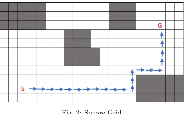
Fig. 3: Square Grid

(19)

2.2 Heuristics

In uninformed search strategies such as Breadth First Search, Depth First Search and Iterative Deepening Search, they do not take the distance to the goal into account. They perform search operations without having any information about reaching the goal state until they stumbled upon one[19]. The heuristic function provides an informed way to guess which neighbour of a node will lead to a goal. It is an estimate of the cost of the optimal(cheapest cost) path from node n to the goal node. The performance of heuristic search is commonly measured by the number of performed node expansions. Some of the commonly used functions for calculating heuristics are Manhattan distance, Euclidean distance and Octile distance.

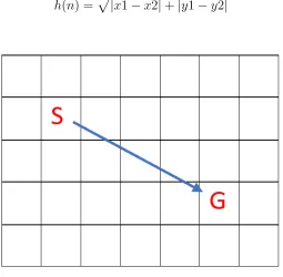
2.2.1 Manhattan Distance

Manhattan distance is often used to calculate the heuristic function for grid-based maps. The movement is restricted to only 4 directions(vertical and horizontal).

Fig. 4: Manhattan Distance

(20)

h(n) =|x1−x2|+|y1−y2| (1)

Manhattan distance provides a good estimate of the time to reach the destination on an open map. However, if the shortest path to the destination is circuitous, then the Manhattan distance becomes a poor estimate.

2.2.2 Euclidean Distance

The Euclidean distance is the straight-line distance between two points in the search space. Since the cost is calculated based on the direct movement by the agent from the starting point to the goal point, Euclidean distance produces accurate results in case of no obstacles. As Euclidean distance is shorter than Manhattan distance or the Diagonal(Octile) distance, we will get shorter paths.

h(n) = p|x1−x2|+|y1−y2| (2)

(21)

2.2.3 Octile Distance

Octile distance is the extension of Manhattan distance that allows diagonal movements[1]. It is commonly used in grid-based maps.

Fig. 6: Octile Distance

The Octile distance is calculated using the following formula,

h(n) = max((x1-x2), (y1-y2)) + (√2−1)∗min((x1−x2),(y1−y2))

For our experiments, we used 1.4 as the value of the square root of 2, as it is the the commonly used value for experiments.

(22)

2.3 A* algorithm

A* is a greedy search algorithm that can be used to find solutions to many prob-lems with pathfinding being one of them. It is the most popular and widely used AI pathfinding informed search algorithm[14]. In a square grid having many obstacles with a given starting node and a goal node, A* finds all the possible paths to reach the goal node. This is done based on certain functions such as g(n), h(n) and f(n).

(23)

the g cost, represented by g(n) and the estimated movement cost to move from the node n to the goal node gives us the h cost, represented by h(n). The sum of the two movement costs g(n) and h(n) gives us the total cost f(n). Based on the f cost, the node which is to be expanded next is chosen. In the A* search, two lists are maintained: the open list and the closed list. The open list stores the nodes that are to be expanded and the closed list stores the nodes that have already been expanded.

In Algorithm 1, the search begins by adding the start node to the open list. The total cost f(n) is calculated by the following formula,

f(n) = g(n) + h(n)

The nodes adjacent to the start node are added to the open list, and the node with the lowest f cost is selected from the open list to be expanded next. The expanded node is then removed from the open list and added to the closed list. While the open list is not empty, the next node with the lowest f cost is selected. If the current node was the goal node, the process terminates and back-traces the path from the goal node to the start node. If the current node was not the goal node, it is removed from the open list and added to the closed list. Then all the possible neighbours of the current node is checked if it is present in the closed list and the open list. If the neighbour nodes are not present in either of the lists, it is then added to the open list and the process continues.

(24)

the time efficiency of the algorithm. In this thesis, we have analyzed the different usages of the data structures and how it has impacted on the results.

2.4 Properties of A* Algorithm

2.4.1 Optimality

There are several search algorithms for solving the problem of pathfinding, but not all the algorithms guarantee finding the least cost path from the start node to the goal node. A* search algorithm always finds all the possible least cost paths from the start node to the goal node. This path is called an Optimal path. If A* returns a solution, that solution is guaranteed to be optimal(least cost) if all the cost esti-mates(heuristics) are optimistic[15]. Among all the optimal algorithms that begins from the start node and uses the same heuristic h, A* expands the minimal number of paths[7].

2.4.2 Admissibility

A search heuristic h(n) is an estimate of the cost of the optimal path from the node n to the goal node. A* is optimal if h(n) is an admissible heuristic, that is, provided that h(n) never overestimates the cost to reach the goal[8][26]. Admissible heuristics are by nature optimistic because it assumes the cost of solving the problem is less than it actually is. Since g(n) is the exact cost to reach n, it is clear that f(n) never overestimates the true cost of a solution through n. The heuristic function h(n) is admissible if for every node n,

h(n)<=h*(n)

(25)

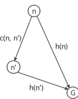
2.4.3 Consistency

A heuristic function h(n) is consistent if for every node n and every successor n’ generated by an action a[18],

h(n) <= c(n,a,n’) + h(n’)

Fig. 7: Consistency Diagram

This is a form of triangle inequality, which depicts that each side of a triangle cannot be longer than the sum of the other two sides. This implies that f(n) never decreases along a path from the root. Considering f* to be the cost of the optimal solution path. A* expands all nodes n with f(n) <f*, and may expand some nodes right on the goal contour before selecting a goal node. The optimality of the A* algorithm can be proved by the following theorems.

Theorem 1If the heuristic is consistent, f value along any path is non-decreasing[7].

(26)

have already been visited and added to the closed list.

Theorem 2 If the heuristic is admissible and consistent, A* could find an optimal

path[7].

The heuristic is said to be admissible when only those nodes whose f values are less(or equal) to the optimal cost path C*, that is, f(n) is less than or equal to C* are expanded. Based on both the theorems, we can prove that our implementation of A* is admissible and consistent, so it provides us an optimal solution.

2.5 A* Operations

The A* algorithm maintains two lists for performing its operations. One is the open list and the other is the closed list. The open list keeps track of those nodes that need to be examined, while the closed list keeps track of those nodes that have already been examined. The open list performs operations such as, insertion, deletion, contains and update. For each iteration, the node with the lowest f-cost is removed from the open list(deletion), and the presence of their neighbour nodes are checked in the open list before adding them(contains). Then those neighbour nodes are added to the open list(insertion). After inserting the nodes to the open list, they are sorted based on the f-cost(update). In this thesis, we focus on how these operations impact on the performance of the A* algorithm.

2.5.1 Open List

(27)

added to the open list. This process is done repeatedly in the main loop until the current node is the same as the goal node.

The performance of the algorithm mainly depends on the number of insertions, deletions, contains and update done in the open list. As the data structures have a major impact on the time complexity of the algorithm, in our research, we have used difference data structures: Min-Heap and Buckets for the implementation of the open and closed list.

2.5.2 Closed List

Comparing to the open list, the closed list does not perform as many operations. The nodes which are expanded are added to the closed list to make sure that those nodes do not have to be expanded again by the agent. Before every insertion of the node in the open list, the closed list is checked for the presence of that node in it. Since the closed list does not perform much operations, it does not necessarily impact the performance of the algorithm.

2.6 Data Structures

In this chapter, we discuss about the various data structures used for the imple-mentation of open and closed list. Among the various data structures, some of the commonly known ones are the array(sorted and unsorted), hash table, Min-Heap and buckets. The time and memory required for performing the operations of the open list determines the efficiency of the A* algorithm. In this thesis, we have used Min-Heap and bucket data structure for the implementation.

2.6.1 Array

(28)

array takes O(1) as it is stored in the last location in the array. For the deletion of the node, it takes O(n) as it has to scan the unsorted array to find the node to be deleted. It takes O(n) for the checking the presence of the node in the open list and updating it, as it has to scan through the array to find the node.

In the sorted array, the number of operations required for inserting a node in the array takes O(n) as it has to sort the array every time a node is added. However, for the deletion of the node, it only takes O(1) because the array is already sorted and the location of the node with the lowest f-cost will be at the end of the array. When we use binary search for checking whether the node is in the array, we require O(log n) operations. If the node is already in the open list, it takes O(log n) to find the node and O(n) to update the node in the list.

2.6.2 Hash Table

In the hash table, the values are stored as index which is a key/value pair. However, in case the keys are larger, we have to convert the large keys into smaller keys by using hash functions. By using the key, we can access the element in O(1) time. Hence insertion of a node will take O(n). Hash tables become quite inefficient when there are collisions; when two keys are hashed to the same slot(index). Due to this collision, the scanning of the array list for the node consumes more time and leads to O(n) operations for removing the node from the array [16].

2.6.3 Min-Heap

(29)

For inserting a node to the heap, the new node should be placed at the last posi-tion just beyond the rightmost node at the bottom level of the tree or as the leftmost position of a new level, if the bottom level is already full. After inserting it at the last position, the value of the new node is compared to the value of its parent node to verify if its value is larger than the parent node. If not, the positions will be swapped. This insertion process takes O(log n).

For removing a node from the heap, we delete the node at the first position(root) of the tree and replace the position with the node at the left position at the bottom-most level. After replacing, we compare the value of the node with its children node to check if the value is smaller than its children. If not, we the positions will be swapped. Hence, the deletion of the node from the heap takes O(log n).

For checking if the open list contains the node, it takes O(n) as it has to scan through the entire tree. If the node is already in the open list, it takes O(n) to find it and O(log n) to update its value in the open list.

2.6.4 Multilevel Buckets

(30)

2.7 Summary

From the above discussions about the various data structures that can be used for the implementation of the open list, it is difficult to narrow down to one specific data structure that would perform well in all the four operations of the open list and the closed list. Each data structure has its own pros and cons in every operation of the open list.

Data Structure Insert Delete Contains Update

Unsorted Array O(1) O(n) O(n) O(n)

Sorted Array O(n) O(1) O(log n) O(n)+O(log n)

Hash Table O(1) O(n) O(1) O(1)

Buckets O(1) O(k) or O(n/k) O(n) O(n) or O(n)+O(n/k)

Min-Heap O(log n) O(log n) O(n) O(n)+O(log n)

Table 1: Time Complexity Comparison of Different Data Structures

In the above table, when we look at the sorted and unsorted array, the insertion operations takes only O(1) in the unsorted array as it is easier to insert a node in an unsorted list whereas it takes O(n) in the sorted array since the array list is sorted every time an element is inserted into the array. However, the deletion operation takes O(n) in the unsorted array and O(1) in the sorted array since in the sorted list, it is easier to locate the element compared to the unsorted list where we need to compare the value of each element to find the lowest valued node.

(31)

seems to take more time to perform insertion and deletion compared to the sorted array, unsorted array and the hash table, which is O(log n).

(32)

Min-Heap and Buckets

3.1 Motivation

Based on our research, we came to know that there are various ways in which pathfind-ing problems can be solved. Different algorithms have been proposed and many improvements have been made to them to optimize the path and reduce the time and space complexities. Some of the popular search algorithms such as Dijkstra’s algorithm and A* algorithm have also been modified to serve this purpose. For our research, we focused on improving the performance of the A* search algorithm. When it comes to A* algorithm, the use of heuristics have made a noticeable improvement in finding optimal(lowest cost) paths. Among the commonly used methods for cal-culating the heuristic function, in our research, we have used Octile distance which gives a shorter path compared to Manhattan distance, as the Octile distance allows the movement of the agent in 8 possible directions(north, south, east, west, northeast, northwest, southeast and southwest), whereas Manhattan distance allows only 4-way movement(east, west, north and south). For our experiment, we have assigned the step cost of diagonal movement to be 14 and the step cost of horizontal and vertical movement to be 10.

(33)

structure has its own advantages and disadvantages, our focus is on Min-Heap and buckets. In the following example, we have taken a square grid with a start node and a goal node.

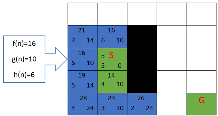
Fig. 8: An example for pathfinding using A* algorithm

In Fig 8, the white nodes represent the traversable(unblocked) nodes and the black nodes represent the block/obstacle in the grid. Initially, we begin our search from the start node that is marked as S in Fig 8. The start node is first added to the open list, and the closed list will be empty. After expanding the start node, the neighbours of the start node are added to the open list if they are not already in the open list, and the start node is added to the closed list as shown in Fig 9. The blue nodes represent the neighbour(adjacent) nodes which are added to the open list. Among the nodes added to the open list, the node with the lowest f cost is selected for expansion.

(34)

As shown in Fig 10, after the node with f value 14 is selected to be expanded, the f values of its adjacent nodes are calculated and added to the open list if they are not already in the open list or the closed list. From the existing nodes in the open list, the node with the smallest f value is again selected for the next expansion.

(35)

This process is continued until the current node is the same as the goal node. Once the current node is the same as the goal node, we return the final optimal(least cost) path found. There are possibility of situations where the obstacles are higher in a map that no path can be found from the start node to the goal node. As we move closer to the goal node, the f cost is increased but the h cost(which is an estimated cost of reaching the goal node from the current node) is decreased.

In Fig 10, the green nodes represent the optimal(least cost) path found from the start node to the goal node. As the agent moves towards the goal, the g cost of the nodes increases while the h cost decreases with becoming zero at the goal node as seen in Fig 11. It can also be seen that there are some nodes which are not expanded in the grid. Since the A* algorithm always chooses the nodes with the lowest f value, the nodes whose f values are much higher will be ignored; it means those paths are longer and costlier to travel.

(36)

path using the A* algorithm that requires a large number of insertions and deletions from the open list and the closed list. For this purpose, a data structure which can reduce the number of operations required for the insertion and deletion has to be used. This motivated us to use the commonly used Min-Heap data structure for A* algorithm and compare it with the Bucket data structure which was mainly intro-duced for the Dijkstra’s algorithm.

When we insert a new node into the open list using the Min-Heap data structure, the node gets added to the last position at the bottom-level of the tree and is then compared with its parent; this process is called up-heap. Likewise, for removing a node from the open list, we perform the down-heap operation where the leaf node is moved to the first position(root) and the node in the root position(node with the lowest f cost) is removed. From this it is clear that the insertion and the deletion operations performed in the open list takes O(log n) using Min-Heap. This led us to consider the bucket data structure where the insertion might take O(1) in the best-case scenario and O(k) for deletion, where k is the size of the bucket. We compared the performance of both the data structures by measuring it based on various factors such as runtime, memory, number of operations and the number of buckets.

3.2 Min-Heap

(37)

3.2.1 Operations of Min-Heap

The four main operations of the open list such as: Insertion, Deletion, Contains and Update, and the two operations of closed list such as Insertion and Contains, can be performed using the Min-Heap data structure.

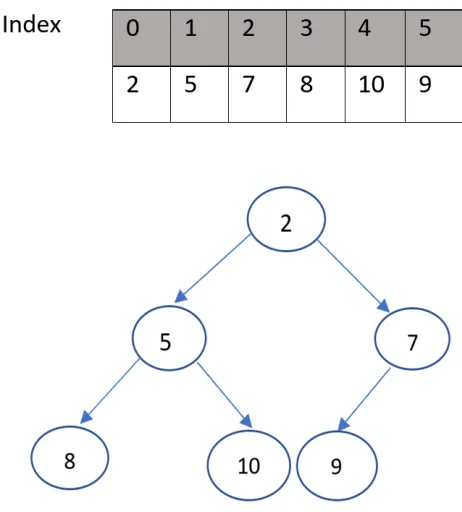
In Fig 12, we have taken an array of 6 elements which will be built into a Min-Heap. The elements in the array are stored in an unsorted manner. Each node has an array index to identify its position. The array index starts from location 0. The first element of the array, 2, is added to the first location of the Min-Heap. When adding the second element of the array to the heap, the second node(child node) is compared to the first node(parent). Since 5 is greater than 2, it is added to the second location in the heap. Likewise, other elements are added to the heap. Every time a node is added/removed from the heap, we check if the value of the current node is greater than its parent node.

(38)

If not, we perform the up-heap operation for insertion and down-heap operation for deletion. In the following we explain in detail how the operations are performed based on Min-Heap data structure.

Insertion:

When inserting a node into the open list, according to the Min-Heap data struc-ture, the new node is added to the position p just beyond the rightmost node at the bottom level of the tree or as the leftmost position of a new level, if the bottom level is already full. Every time a new node is added to the last position of the tree, its f cost is compared to the f cost of its parent. Min-Heap is a complete binary tree, where the parent node should always be smaller than its children nodes. When the condition is not satisfied, the position of the parent node gets switched with its child node. This swapping is continued until the condition is met.

Fig. 13: Example of Min-Heap data structure

(39)

node, the positions of both the nodes will be swapped. In the above example, since the child(12) is greater than its parent(7), the position of the nodes will remain the same. If the child node was smaller than the parent node, the child node’s position would have been swapped with the parent node and the current child node will again be compared with its parent node. This takes O(log n) operations for inserting the new node to the end of the heap as a leaf node and comparing its value to its parent node and swapping positions until it satisfies the condition of the binary tree.

Deletion:

When deleting a node from the heap, the leaf node at the last position p at the rightmost position at the bottom-most level of the tree is removed. To preserve the entry from the last position p, we add it to the root r of the tree. The value of the current node added to the root of the tree is compared to the value of its child node. If the value of the current node is greater than the child node, the positions of both the nodes get swapped. This process is continued until the tree satisfies the conditions of the binary tree.

(40)

from the tree and the first position is replaced with the element 12 from the last bottom-most position of the tree.

After replacing, the down-heap operation is performed where the parent node is compared to the child node to check if the parent node is lesser than its child node as shown in Fig 15 and Fig 16. This is continued until the heap satisfies the condition.

(41)

Based on the down-heap operation, the check is performed for verifying the values of the parent node and the child node. In Fig 15, since the value of the node in the first position, 12, is greater than its child node, which is 5, their positions get swapped in the tree. Then the current node, 12, is again compared with its child nodes whose values are 8 and 10. Since it is greater than the child node, the positions get swapped again until we get a binary tree.

The deletion operation takes O(log n) operations to remove a node from the tree as it has to remove the first node of the tree and replace its position with the node from the bottom-most level of the tree, and compare the values of the nodes with its child nodes and perform swapping wherever necessary.

Contains:

(42)

is done by comparing the node to the already existing nodes in the heap with the help of some attributes like a pointer to its predecessor or a specific location of the node in the map. If the node is not present, we then add the node to the heap. This operation takes O(n) as it has to check the entire tree from top or from bottom to locate the node we are searching for.

U pdate:

In the update operation, we check the heap for the existence of the node in the data structure and update its value if its value is smaller than the existing value. We search for the node in the heap(contains) and replace the node with the updated new value which is lesser than the current value. That is, we perform the contains operation for finding the current node in the tree and when the node is found, we compare the value of the current node with the already existing node. If the value of the current node is lower than the value of the already existing node(duplicate) node, we replace or update the node with its new lowest value.

This operation is expensive compared to the other operations of the open list, as it involves searching for the node in the entire tree(contains) and then updating the value of the node with its new lowest value found. The contains operation takes O(n) and updating its value takes O(log n).

3.3 Buckets

(43)

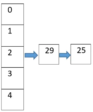
As an example, we have taken an unsorted array of 8 elements which are as-sumed to be the f values of the nodes we come across while searching for the final optimal(least cost) path based on the A* search algorithm using the bucket data structure. As shown in Fig 16, we have an unsorted array of 8 elements(0-7) which will be added to the buckets. For these 8 elements we have taken 5 buckets with each bucket holding values of different ranges.

Suppose, the first bucket will store values between 0 and 10, second bucket will store the values between 11 and 20 and so on. The bucket size keeps growing based on the number of values present within the chosen range for each bucket. Like the Min-Heap data structure, the four operations(insert, delete, contains and update) of the open list are also performed using buckets. In the following, we discuss in detail about the four operations.

(44)

Insertion:

As we know, the operation of insertion is to insert a new node which has the possi-bility to be expanded, into the open list. We created different buckets for storing the nodes, with each bucket holding a certain range of values it allows the nodes to be inserted. Arraylists were created for storing the nodes in the buckets as it does not require a fixed size to be declared when creating an object. Every time a node is to be inserted into a bucket, we calculated the position of the bucket where the node should be inserted based on the bucket interval.

Fig. 19: Example of Bucket data structure

(45)

As shown in Fig 18, we have an unsorted array of 8 elements. We created 5 buck-ets for storing these 8 elements. The first bucket stores the values between 0 and 10, the second bucket stores values between 11 and 20 and so on. The first element of the array, 29, is added to the third bucket as it falls between the range 21-30, as shown in Fig 20. Likewise, the second element of the bucket, 25, is added to the third bucket which holds the range 21-30. Since the insertion of the node into the open list is straight forward(no swapping is required) by buckets, it only takes O(1) operations for inserting a new node into the bucket.

The nodes can also be stored separately in buckets with one node in each bucket. But storing the nodes this way would require a larger number of buckets when deal-ing with large sized maps. Instead, we can set a range of values based on the f values of the nodes to store the nodes falling under the range. Either way, the insertion in the bucket takes less operations compared to the Min-Heap.

Deletion:

(46)

the node into the open list, it takes O(1) operations as we do not have to perform the bubble-up process like in Min-Heap for sorting the list. Whereas, when removing the node from the list, we need to scan through the array to find the node with the lowest f value if the bucket has more than one value stored in it. This operation takes O(k), where k is the size of the bucket. This k depends on the number of nodes added to the bucket and the number of buckets used.

However, the operations required for deletion of the node from the open list in buckets is still cheaper than the Min-Heap, where it requires O(log n). For example, in Fig 20, the nodes in the buckets are not sorted. So when deleting the least cost node from the bucket, we need to scan the array to find the node as shown in Fig 20. In the third bucket, there are 3 nodes: 29, 25 and 21. Among the 3 nodes, 21 will be removed as it is the least cost. For removing 21 from the list, it will take O(3) as the bucket size is 3.

Contains:

(47)

update operation will be performed for updating the value. This Contains operation takes O(n) to scan through the buckets to find the node. The number of operations required for performing this Contains operation is O(n) for both the data structures, Min-Heap and Buckets.

This bucket data structure was mainly introduced for solving the problems of Di-jkstra’s algorithm which does not perform the contains operations as it is performed in A* algorithm.

U pdate:

Update operation is performed for updating the f value of the already existing node in the bucket. Initially, we need to locate the node in the buckets for which we are updating the value. The existence of the node in the bucket is first checked by per-forming the contains operation and getting the position of the node in the bucket. After finding the node, we compare the f values of the current node to the already existing node(duplicate). If the value of the current node is lesser than the value of the existing node, its value will get replaced.

This shows that the updating of the node in the bucket requires performing the scanning(contains) first and then replacing the values of the node in the bucket. For the scanning of nodes in the bucket, it requires O(n) operations and then replacing the value of the node in the bucket takes O(log n), since after the value of the node is updated, the nodes in the bucket have to be sorted based on the new lowest value.

3.4 Summary

(48)

(49)

Experiments and Results

4.1 Implementation Specifications

The implementation and testing of our project was done using Java and Eclipse IDE. The main goal of our thesis is to compare the different data structures for imple-menting the open list in the A* algorithm. We began by setting the start node and the goal node in a random map with obstacles, where the agent has to find the least cost path from the start node to the goal node. Among the several search algorithms for pathfinding, we chose to perform our research on the A* algorithm which is the most popular informed search algorithm. This algorithm maintains two lists, open list and the closed list. The operations performed in these two lists determines the performance of the algorithm.

(50)

4.2 Experimental Setup

For our thesis, we performed our implementations on squared-grid maps as it pro-duces better results. In our environment, the agent is allowed to move in 8 di-rections(horizontal, vertical and diagonal). The movement cost for horizontal and vertical movement is 10, and the diagonal movement cost is 14. The heuristics were calculated using the Octile distance.

Fig. 22: Map Size 512x512

(51)

parameter to vary.

4.2.1 Search Parameters

Before running our experiments, we first need to determine the different map sizes we are going to be using to run our tests. Secondly, we need to determine the percentage of obstacles in the maps. We have used maps of sizes ranging between 40x40 and 560x560. Through our experiments, we found that when the percentage of obstacles goes above 40 percent, the chances of finding a path from the start node to the goal node reduces. Hence, we varied the obstacle percentages between 0% to 40% in our maps. In our system, we have made the start node and the goal to be manually changed and varied obstacle densities for every map. Since we are going to be com-paring the performance of different data structures for implementing the open list of the A* search, there are certain factors we need to consider. Min-Heap and buck-ets are the two data structures we are going to be comparing and running our tests on.

The parameters we need to consider when comparing the performance of two data structures can be the different sizes of maps, the percentage of obstacles in the map, the number of operations each data structure takes for performing insert, delete, con-tains and update, the time taken to find the least cost path, the number of nodes expanded for finding the least cost path, the memory required for the open list and the closed list etc. Additionally, we have made it possible in our system to change the number of buckets used for storing the nodes in the open list. This is one of the important parameters to consider when calculating the operations required for inser-tion and deleinser-tion of nodes using bucket data structure. Based on these parameters, we ran our tests in different data structures separately.

(52)

4.3 Performance Evaluation

For comparing the different data structures based on certain parameters, we gathered the results of the time taken to run the algorithm using different data structures, the number of nodes expanded and added to the closed list, the length of the path found from the start node to the goal node, the number of operations performed by the open list and the closed list and the memory required for storing the lists(maximum size of the open list and the closed list).

4.3.1 Time

Time is evaluated based on the duration taken to complete the process of finding the least cost path beginning from the start node to the end of reaching the final node and returning the optimal(least cost) path found. Determining the time taken to find the path shows the efficiency of the search algorithm. As we have implemented our algorithm in Java, the execution time may have some variations each time we run the program.

(53)

The java performance may get affected by the applications running in the back-ground, as well as by the VM(Virtual Machine) driven by the JIT(Just In Time) optimizer, garbage collection, thread scheduler, etc[12]. To get a precise execution time we have to shut down all the other processes running in the background and run our program a couple of times. We ran our program with the same parameters for about 30 times to get an average execution time. As shown in Fig 23, the execution time reduced from 1800ms and maintained between 1500ms and 1600ms after running the program for more than 10 times. We tested this with the same parameters for different data structures, and for both the data structures the execution time was higher for the first 5 times we ran the program and then maintained the average runtime for the remaining times.

4.3.2 Number of Nodes Expanded

As we have implemented the A* algorithm using different data structures, we have considered the different parameters to look at when determining the performance of the data structures. Keeping track of the number of nodes expanded is one of the factors to be considered, as the A* algorithm will always choose the best node with the lowest f value in the open list. Based on the efficiency of the data structures, the number of nodes expanded may vary and it may affect the number of operations it takes. However, since we use the A* algorithm, we do not require to check the number of nodes in the final path, as the number of nodes in the final path will always be the same. We have used the same parameters for both the data structures and kept track of the number of nodes in the open list and the closed list.

4.3.3 Path Length

(54)

of consistency and admissibility. Although this parameter seem to be not quite re-quired to evaluate the data structures, it will still be useful for verifying the results produced. As the nodes in the final path will be the same for both the data structures.

Fig. 24: Path length of the data structures

Since the path does not change for different data structures, we can verify after running the program if both the data structures have produced the same path. This way the path length can be considered as a necessary parameter for performance evaluation.

4.3.4 Number of Operations

(55)

In the Min-Heap data structure, the insert operation of the open list takes O(log n) times as the node is inserted at the last position of the bottom-most level of the tree and it has to perform bubble-up operation to satisfy the condition of the binary tree: the parent node should always be smaller than the child nodes. Similarly, the delete operation takes O(log n) for deleting the node with the lowest f value in the open list as it performs the bubble down process. As for the contains, we compare the current node with the nodes in the open list to avoid duplicate node to be inserted into the open list. This takes O(n) operations for checking the entire tree to locate the node we are searching for. The update operation is called O(n) for checking the entire tree for the node and O(log n) for updating the f value of the node if found.

For the bucket data structure, the insertion of node into the open list is quite straight-forward as it does not have to perform bubble-up as in Min-Heap. Therefore it takes O(1) for performing insertion in the buckets. However, deletion of the node from the open list takes O(k) operations, where k is the size of the bucket . The size of the buckets are not fixed as it depends on the number of buckets used and the f values of the nodes. For insertion, we insert the nodes into an unsorted arraylist, whereas, for deleting in order to remove the node with the lowest f value, we scan through the list to remove the node with the lowest f value at the head of the list since the A* algorithm performs the deletion of node from the open list by first in first out(FIFO) method. However, the number of operations required for deleting the node from the open list by buckets is still lesser than Min-Heap where it takes O(log n).

4.3.5 Number of Buckets

(56)

at the insertion of the nodes into the open list, the nodes are inserted into the bucket in unsorted manner. Even if we increase or reduce the number of buckets used, it will still take only O(1) operations for inserting the node. On the other hand, for deletion, the number of operations may vary based on the number of buckets used as the size of the bucket increases based on the total number of nodes added to the bucket.

The performance of the bucket can be measured by varying the size of the bucket(k). Based on the map sizes and the obstacle density, varying the size of the bucket might be useful in finding the optimal size of the bucket, which might improve its perfor-mance.

4.4 Results and Analysis

For measuring the performance of the data structures, we ran our tests in maps of different sizes and varied the percentage of obstacles in every map. The sizes of the maps that we generated are ranging from 40x40 to 560x560. The start node and the goal node was chosen randomly in each map and we set the start and the goal node as far as possible, and maintained the same start node and the goal node for every test we ran in different maps with different obstacle percentages to be fair. Since the distance between the start and goal node has major impact on the time taken and the number of operations. We compared the results of the two data structures, Min-heap and Bucket, with the same map specifications.

(57)

path became harder. The results of the tests were compared based on the number of operations, runtime, memory usage and the obstacle density.

4.4.1 Runtime

Fig. 25: Runtime of Map Sizes from 40x40 to 300x300

(58)

For calculating the runtime, we ran the tests on the maps that we generated by varying the percentage of obstacles in it. The runtime was calculated based on the duration taken to find the least cost path from the beginning of the start node to the end of reaching the final node and returning the least cost path that was found. The tests were performed on both the data structures with the same specifications(start node, goal node, obstacle percentage and map size).

Fig. 26: Runtime of Map Sizes from 360x360 to 560x560

(59)

changed the start node and the goal node with 0% obstacles, and ran our tests a couple of times again to verify if this was the reason.

As we increased the size of the map in our test environment, the time taken for finding the least cost path also increased. We added the length of the final path which was found since it was useful in determining the correctness of the results pro-duced by the two data structures, as the A* search algorithm finds the least cost path irrespective of the data structure used for creating the open and closed lists. For example, the path length of the least cost path for the map 520x520 in Fig 25 is 381 for both the data structures.

Fig. 27: Runtime of Map Size: 40x40 with Obstacles: 5% to 40%

(60)

ob-stacle percentage went above 50%. When we increased the percentage of the obob-stacle to 40%, the min-heap data structure took the maximum time for the 40x40 map. As the path length increased, the runtime also got longer.

We noticed that in almost all the cases, the bucket data structure performed bet-ter than the min-heap. It was also noted that the differences in runtime between the data structures were smaller in the 40x40 map with 5% to 30% obstacles, but it increased only when the obstacle percentage increased to 40%.

Fig. 28: Runtime of Map Size: 200x200 with Obstacles: 5% to 40%

(61)

As shown in Fig 28, the number of operations taken to find the least cost path in a 200x200 map with 0% obstacles is approximately 85000. This number was increased when the obstacle percentage was 40% and hence took longer runtime. When running the tests on larger maps, we found that the difference in the runtime between the two data structures was huge as the map size was bigger, and the bucket data structure was performin much better compared to min-heap.

Fig. 29: Runtime of Map Sizes: 40x40 to 560x560

(62)

Similar tests were run for 512x512 map with obstacle percentage ranging between 5% to 40%. The time taken for finding the least cost path was varying based on the map structure and the obstacle density. When we look at Fig 29, the runtime for map with 15% and 20% obstacle density was higher than when there was 25% obstacle density, this is due to the selection of the start node and the goal node, and the obstacles in between them.

Obstacle Percentage Heap Runtime(ms) Bucket Runtime(ms) Path Length

5% 105 92 38

10% 125 120 54

30% 238 235 66

40% 398 345 72

Table 2: Runtime Comparison of 40x40 Map With Different Obstacle Density

When the obstacle density was 15%, there might have been much obstacles in the path towards the goal node but not the surrounding places, so the algorithm might have to look for traversal nodes which might have taken longer time for calculating and finding the least cost path.

Obstacle Percentage Min-Heap Runtime(ms) Bucket Runtime(ms) Path Length

5% 17970 16063 166

10% 18348 17320 166

30% 19728 18521 145

40% 20891 20211 251

(63)

structures, we can say that the time taken for finding the optimal(least cost) path was much higher when the obstacle density was increased to 40% and the path length was also higher compared to the other maps. However, in every test, it was clear that the Min-Heap was taking more time in finding the least cost path compared to the Buckets. This might be the result of the number of operations being performed by the Min-Heap, which are lesser when using Buckets.

Fig. 30: Runtime of Map Size: 512x512 with different Obstacle Density

(64)

Obstacle Percentage Min-Heap Runtime(ms) Bucket Runtime(ms) Path Length

10% 309566 297595 234

15% 583756 529474 243

20% 606026 400064 256

25% 439189 431343 238

30% 499060 347583 240

35% 662399 628840 260

40% 980071 912960 300

4.4.2 Number of Operations

Since calculating the runtime alone was not sufficient to come to a conclusion of which data structure was performing better, it is also required to measure the performance of the data structures based on the various factors which could affect the execution of the runtime[12]. We calculated the number of operations taken by the data structures for performing the operations of the open list. We counted the number of operations of the open list: insert, delete, contains and update, and totalled it to get the total number of operations performed by each data structure.

(65)

Fig. 31: Number of Operations of Map Sizes: 40x40 to 300x300

(66)

parent node to check if the parent node is smaller than the child node. This process involves more than one number of swapping. Therefore, for each insertion or deletion, there might be multiple number of swapping performed.

Fig. 32: Number of Operations of Map Sizes: 360x360 to 560x560

(67)

Obstacle Percentage Min-Heap Operations Bucket Operations Path Length

5% 377591 205683 163

10% 376155 239907 156

30% 401502 325608 175

40% 402834 347826 178

Table 5: Number of Operations of 280x280 Map With Different Obstacle Density

When conducting these tests, we found that the number of operations for Con-tains was almost the same in both the data structures, buckets and min-heap. This is because, in the Contains operation, the existence of the current node in the open list or the closed is checked by comparing it to each node present in the open list and the closed list. Table 5 shows the number of operations taken by the Min-Heap and the Buckets in a 200x200 map with different obstacle density ranging between 5% to 40%.

(68)

The same operations(insert, delete, contains and update) are performed using both Min-Heap as well as Buckets. Therefore, the major difference in the total num-ber of operations taken by the data structures is due to the numnum-ber of insertion and the number of deletions performed. The insertion in the buckets is straight forward, whereas in the min-heap it has to perform the swapping(upheap for insertion and down heap for deletion). However, for the deletion, the buckets are scanned in order to find the node with the lowest f cost in the open list. Therefore, the total number of operations are also higher in the min-heap compared to the buckets.

In Fig 33, it is clear that the number of operations taken by the Min-Heap grew larger as the size of the map grew larger. Whereas, with the Buckets, the number of operations did not take such drastic changes. The total number of operations(insert, delete, contains and update) taken by the two data structures are shown in Table 6 along with the length of the final path for different density of obstacles in the map.

Fig. 34: Number of Operations of Map Size: 512x512 with Obstacles

(69)

operations taken between the data structures were smaller compared to the Fig 34, where when the map size was 520x520 and 560x560, the difference was huge. The de-tailed number of operations taken by each data structures is shown in Table 6. From the table and the graphs, we can see that the Bucket data structure was using lesser number of operations for performing the operations of the open list and the closed list compared to the Min-Heap. We verified this by running our test in different map sizes with different obstacle densities. We set the same start node and goal node for both the data structures.

Obstacle Percentage Min-Heap Operations Bucket Operations Path Length

10% 482204 427879 234

15% 518670 502438 243

20% 696802 618670 256

25% 627879 602246 238

30% 505968 460863 240

35% 627879 599030 260

40% 771274 734268 300

Table 6: Number of Operations of 512x512 Map With Different Obstacle Density

4.4.3 Memory

(70)

As shown in Fig 35, the size of the open list is the same for Min-Heap and Buckets, though it is lesser than the size of the closed list. There was a difference of one or two in the open list and the closed list between both the data structures, but it can be ignored as it was very small. This is due to the fact that both the data struc-tures followed the Last In First Out(LIFO) rule where the redundant nodes were not traversed[4]. In majority of the cases, the size of the open list was smaller than the size of the closed list. However, there were times when the size of the open list was almost the same as the size of the closed list.

(71)

As the size of the map grew bigger, the maximum size of the open list and the closed list also got bigger as the distance between the start node and the goal node would be larger so it has to expand more nodes, which is, adding more nodes to the open list and the closed list.We verified the results by checking the length of the final path found by the Min-Heap and the Buckets.

Fig. 36: Memory required for Map Sizes: 360x360 to 560x560

(72)

oper-ations performed by each data structure.

The differences in the memory requirement of the data structures were not high when we ran our tests on smaller sized maps, as the number of nodes expanded would be less. So, we ran the tests on larger maps like 480x480 and 560x560, as shown in Fig 36, in which the differences between the memory requirement of the open list and the closed list was larger. Sometimes the differences in the memory requirement for the open list and the closed list were almost the same or close enough depending on the optimal(least cost) path which was chosen.

Fig. 37: Memory required for Map Size: 512x512 with different Obstacle Density

(73)

However, in the closed list, when the obstacle percentage was 10%, 20% and 35%, the difference in the memory requirement between the data structures were larger.

Fig. 38: Memory required for Map Size: 512x512 with different Obstacle Density

The memory requirement of the closed list was considerably lesser when the ob-stacle percentage was 25%. Whereas, when we increased the obob-stacle density to 30% and 40%, the memory requirement of the closed list became much higher. This can be due to the different paths to traverse when finding the optimal(least cost) path. That is, since the percentage of obstacles became higher, it got more difficult to find the optimal(least cost) path, so the agent has to traverse through redundant nodes to find the final path.

4.5 Summary

(74)

(75)

Conclusion

In this thesis, among the several search algorithms introduced for pathfinding, we fo-cused on improving the performance of the A* search algorithm. While we explored the different ways for improving the performance of the A* algorithm, we found that the A* algorithm for pathfinding was affected by the data structures used for im-plementing the open lists. The commonly used data structure for imim-plementing the open list is the Min-Heap. The insertion and deletion operations in Min-Heap takes O(log n) times to insert nodes into the open list and O(log n) times to delete the nodes from the open list as it has to perform bubble-up and bubble-down process for satisfying the conditions of the binary tree.

(76)

node with lowest value. However, the contains operation takes O(n) for both the data structures. We considered the various factors for evaluating the performance of the data structures such as time, number of nodes expanded, number of buckets used, path length and the number of operations. Based on these factors we compared the results to find which data structure was performing better with A*.

In our experiments, we differed the sizes of maps and the percentage of obstacles in the map and found that the possibility of finding a path from the start node to the goal node becomes harder when we increase the percentage of obstacles above 40 percent. The path found using the Min-Heap and buckets were also the same under the same parameters used, but the number of nodes expanded by the buckets was one lesser than the Min-Heap. We ran our tests a number of times to find the average execution time of finding the path from the beginning of the search till finding the final node and returning the path.

(77)

Future Work

For our thesis, we found better heuristics by allowing the agent to move in 8 directions by setting the horizontal and vetical cost as 10 and the diagonal cost as 14. Addition-ally, for improving the performance of the A* algorithm in terms of the operations performed in the open list, we used the bucket data structure. Although the buckets produced better results compared to the Min-Heap, the number of operations taken for deleting the node from the open list can grow significantly high for larger maps. In this case, the overall performance of the data structure may get affected and may lead to Min-Heap outperforming the buckets.

(78)

[1] Yngvi Björnsson and Kári Halldórsson. Improved heuristics for optimal path-finding on game maps. AIIDE, 6:9–14, 2006.

[2] Adi Botea, Bruno Bouzy, Michael Buro, Christian Bauckhage, and Dana Nau. Pathfinding in games. Schloss Dagstuhl-Leibniz-Zentrum fuer Informatik, 2013.

[3] Adi Botea, Martin M¨uller, and Jonathan Schaeffer. Near optimal hierarchical path-finding. Journal of game development, 1(1):7–28, 2004.

[4] Qing Cao. Exploiting problem structure in pathfinding. 2018.

[5] Xiao Cui and Hao Shi. A*-based pathfinding in modern computer games. IJC-SNS, 11(1):125, 2011.

[6] Xiao Cui and Hao Shi. An overview of pathfinding in navigation mesh. IJCSNS, 12(12):48–51, 2012.

[7] Rina Dechter and Judea Pearl. The optimality of a* revisited. In AAAI, pages 95–99, 1983.

[8] Rina Dechter and Judea Pearl. Generalized best-first search strategies and the optimality of a. Journal of the ACM (JACM), 32(3):505–536, 1985.

[9] Samuel Erdtman and Johan Fylling. Pathfinding with hard constraints: Mobile systems and real time strategy games combined, 2008.

(79)

Pha*: finding the shortest path with a* in an unknown physical environment.

Journal of Artificial Intelligence Research, 21:631–670, 2004.

[11] George HL Fletcher, Hardik A Sheth, and Katy B¨orner. Unstructured peer-to-peer networks: Topological properties and search performance. In International Workshop on Agents and P2P Computing, pages 14–27. Springer, 2004.

[12] Andy Georges, Lieven Eeckhout, and Dries Buytaert. Java performance evalua-tion through rigorous replay compilaevalua-tion. In ACM Sigplan Notices, volume 43, pages 367–384. ACM, 2008.

[13] Andrew V Goldberg and Craig Silverstein. Implementations of dijkstras algo-rithm based on multi-level buckets. In Network optimization, pages 292–327. Springer, 1997.

[14] Peter E Hart, Nils J Nilsson, and Bertram Raphael. A formal basis for the heuristic determination of minimum cost paths. IEEE transactions on Systems Science and Cybernetics, 4(2):100–107, 1968.

[15] Patrik Haslum, Blai Bonet, H´ector Geffner, et al. New admissible heuristics for domain-independent planning. In AAAI, volume 5, pages 9–13, 2005.

[16] Ward Douglas Maurer and Theodore Gyle Lewis. Hash table methods. ACM Computing Surveys (CSUR), 7(1):5–19, 1975.

[17] Colin JH McDiarmid and Bruce A. Reed. Building heaps fast. Journal of algo-rithms, 10(3):352–365, 1989.

[18] Masoud Nosrati, Ronak Karimi, and Hojat Allah Hasanvand. Investigation of the*(star) search algorithms: Characteristics, methods and approaches. World Applied Programming, 2(4):251–256, 2012.

(80)

[20] Li-Yen Shue and Reza Zamani. An admissible heuristic search algorithm. In

International Symposium on Methodologies for Intelligent Systems, pages 69–75. Springer, 1993.

[21] Nathan R Sturtevant. Benchmarks for grid-based pathfinding. IEEE Transac-tions on Computational Intelligence and AI in Games, 4(2):144–148, 2012.

[22] Nathan R Sturtevant. Choosing a search space representation. Game AI Pro: Collected Wisdom of Game AI Professionals, 1:253–258, 2013.

[23] Anders Strand-Holm Vinther, Magnus Strand-Holm Vinther, and Peyman Af-shani. Pathfinding in two-dimensional worlds. no. June, 2015.

[24] Ko-Hsin Cindy Wang, Adi Botea, et al. Fast and memory-efficient multi-agent pathfinding. InICAPS, pages 380–387, 2008.

[25] F Benjamin Zhan. Three fastest shortest path algorithms on real road networks: Data structures and procedures. Journal of geographic information and decision analysis, 1(1):69–82, 1997.