Dynamic Time Series Analysis Using Logistic Function

ABSTRACT

SangPil Hwang. Dynamic Time Series Analysis Using Logistic Function. (Under the

direction of David A. Dickey.)

This paper investigates a set of autoregressive time series models whose coefficients

have the form of a logistic function. The transfer function type models give additional

flexibility over the fixed coefficients models and include them as a special case. NLAR

models with the AR(1) coefficient being a hyperbolic tangent function work well for

modeling series which have asymmetric stochastic volatility or changing amplitude

Dynamic Time Series Analysis Using Logistic Function

by

SangPil Hwang

A dissertation submitted to the Graduate Faculty of North Carolina State University

in partial fulfillment of the requirements for the Degree of

Doctor of Philosophy

STATISTICS

Raleigh

2004

APPROVED BY:

David A. Dickey Sastry G. Pantula

Chair of Advisory Comittee

Biography

SangPil Hwang was born in ChangWon, the Republic of Korea on Feburary 1, 1967.

He entered Department of Economics at Seoul National University in 1985 and took

his B.S. in Economics in 1989. He worked for the Bank of Korea from 1992 to 2000.

He joined Department of Statistics, North Carolina State University for the pursuit

Acknowledgements

I would like to express my deepest gratitude and biggest appreciation to my advisor

Dr. David A. Dickey. I am also grateful for precious instruction and helpful

sugges-tions from Dr. Sastry G. Pantula, Dr. Bibhuti B. Bhattacharyya and Dr. Matt Holt.

Contents

List of Tables vi

List of Figures vii

1 Introduction 1

2 Transfer function type models 13

2.1 some nonlinear models . . . 13

2.2 simulation . . . 41

2.3 application . . . 43

3 Nonlinear autoregressive model 94 3.1 NLAR(1) model . . . 94

3.2 simulation . . . 117

3.3 further analysis . . . 123

3.4 application . . . 129

4 Conclusion 205

List of Tables

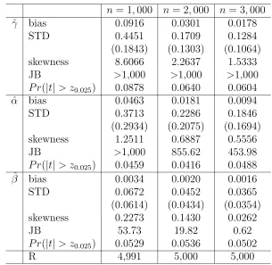
2.1 Distribution of ˆγ,α,ˆ and ˆβ for model (2.1) . . . 66

2.2 The summary of yearly precipitation and stream flow(1949-2001) . . . 68

2.3 Major Hurricane or tropical storm passing through both regions . . . 69

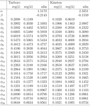
2.4 The coefficient estimates from the fitted models . . . 70

3.1 Estimation of α and β for model (3.1) where f(y) = y . . . 150

3.2 Distribution of ˆα and ˆβ for model (3.1) where f(y) = y . . . 153

3.3 Comparison of ARMA and nonlinear estimation for model (3.1) where f(y) = y . . . 157

3.4 Estimation of α and β for model (3.1) where f(y) = |y| . . . 159

3.5 Distribution of ˆα and ˆβ for model (3.1) where f(y) = |y| . . . 162

3.6 Comparison of ARMA and nonlinear estimation for model (3.1) where f(y) = |y| . . . 166

3.7 The distribution of ˆα and ˆβ whereβ = 0 n = 1,000 . . . 168

3.8 Distribution of ˆα and ˆβ for model (3.2) where f(y) = y . . . 169

3.9 Distribution of ˆα and ˆβ for model (3.2) where f(y) = |y| . . . 173

3.10 The mean of model (3.1) with γ = 0.99, 0.999 and 1.00, α = 1.0, and β = 0.8 . . . 177

3.11 Estimation of α and β with γ fixed at 0.99 wheref(y) = y . . . 179

List of Figures

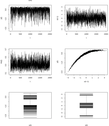
2.1 y_t and x_t where (a) (γ, α, β, σ) = (1.0,0.8,0.5,0.04) . . . 72

2.2 y_t and x_t where (b) (γ, α, β, σ) = (1.0,−1.0,−0.8,0.04) . . . 73

2.3 (a) the log transformed stream flow series of Goldsboro(dotted line) and

Kinston(solid line), (b) prediction(dotted line) and actual series(solid

line) for Kinston . . . 74

2.4 The cross-correlation of ∇y_t and ∇x_t . . . 75

2.5 (a) the log transformed stream flow series of Goldsboro, (b) ρ(dx_t−2)

vs time, (c)1−ρ(dx_t−2) vs time . . . 76

2.6 (a) phase spectrum and (b) squared coherency of two log transformed

stream flow series at a high flow period(solid line) and a low flow

pe-riod(dotted line) . . . 77

2.7 The response deviations and the changes in ρ(dx_t−2) from the

equi-librium state by the given impulse of (a) AR(1), (b) AR(2), and (c)

AR(5), at a high flow(solid line) and a low flow(dotted line) . . . 78

2.8 (a) the log transformed stream flow series of Kinston(dotted line) and

Fort Barnwell(solid line), (b) prediction(dotted line) and actual

se-ries(solid line) for Fort Barnwell . . . 79

2.9 (a) the cross-correlation of∇y_t and∇x_t, (b) the cross-correlation ofy_t

and x_t . . . 80

2.10 (a) 1−ρ₁(dx_t−2)−ρ₂(dx_t−2) vs time, (b)ρ₁(dx_t−2) vs time, (c)ρ₂(dx_t−2)

vs time . . . 81

2.11 SOI and recruitment series . . . 82

2.12 Scatterplot of recruitmenty_twith lagged SOI data,x_t−h, h= 0,1,4· · ·,10 83

2.13 The cross-correlation of y_t and x_t . . . 84

2.14 (a) ρ(x_t−5) vs time, (b) ρ(x_t−5) vsx_t−5 . . . 85

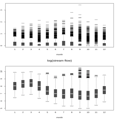
2.15 Boxplot of rainfall and stream flow in Tarboro(on a daily basis) . . . 86

2.16 Boxplots of rainfall and stream flow in Kinston(on a daily basis) . . . 87

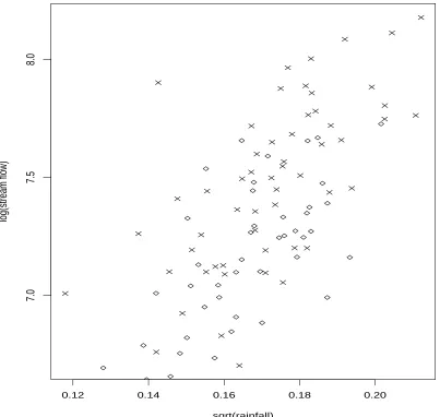
2.17 Scatterplot of yearly rainfall and stream flow in Tarboro and

Kin-ston(daily average): ♦ Tarboro and× Kinston . . . 88

2.18 QQ plots of rainfall and stream flows in Tarboro and Kinston . . . . 89

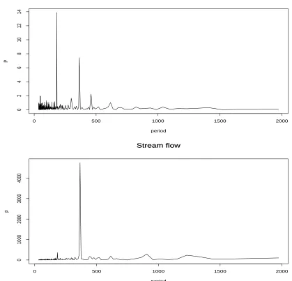
2.20 Periodograms of rainfall and stream flows in Kinston . . . 91 2.21 The cross-correlations of rainfall and stream flows in Tarboro(solid line)

and Kinston(dotted line) . . . 92

2.22 The phase spectrum of rainfall and stream flows in Tarboro and Kinston 93

3.1 y_tandρ(y_t−1) of series generated by (a) (γ, α, β) = (0.99,1.0,0.8) where

f(y) = y . . . 181

3.2 y_t and ρ(y_t−1) of series generated by (b) (γ, α, β) = (0.99,−3.0,0.1)

wheref(y) =y . . . 182

3.3 y_t and ρ(y_t−1) of series generated by (c) (γ, α, β) = (0.99,−1.0,−1.2)

wheref(y) =y . . . 183

3.4 y_t and ρ(y_t−1) of series generated by (d) (γ, α, β) = (0.99,1.0,0.8)

wheref(y) =|y|. . . 184

3.5 y_t and ρ(y_t−1) of series generated by (e) (γ, α, β) = (0.99,−3.0,0.1)

wheref(y) =|y|. . . 185

3.6 y_t and ρ(y_t−1) of series generated by (f) (γ, α, β) = (0.99,−1.0,−0.8)

wheref(y) =|y|. . . 186

3.7 Examples of series generated by (γ, α, β, σ) = (0.99,0.8,0.45,0.1)

un-der (a)η_t=e_t (b) η_t= 0.95η_t−1 +e_t where f(y) =y . . . 187

3.8 The trend of mean withσ2 = 1.0 where f(y) = y . . . 188

3.9 The trend of mean withσ2 = 0.25 where f(y) = y . . . 189

3.10 The areas where t tests of α = α₀ and β = β₀ have empirical

re-jection rates not significantly different from 0.05 based on binomial

test. f(y) = y and nonlinear estimation convergence rates bigger than

99.5%; (a) σ= 1.0 and (b) σ= 0.5 . . . 190

3.11 The areas where t tests of α = α₀ and β = β₀ have empirical

rejec-tion rates not significantly different from 0.05 based on binomial test.

f(y) = |y| and nonlinear estimation convergence rates bigger than

99.5%; (a) σ= 1.0 and (b) σ= 0.5 . . . 191

3.12 The trend of y_t and ρ(y_t−1); (a)c= 4.0, (b)c= 1.0, (c)c= 0.0. From

the left, γ = 0.9, γ = 1.0. For ρ(y_t−1), the solid line is at γ = 0.9 and

the dotted line is at γ = 1.0. . . 192

3.13 The trend of y_t and ρ(y_t−1); (d) c=−0.2, (e) c=−1.0, (f) c=−4.0.

From the left,γ = 0.9, γ = 1.0. Forρ(y_t−1), the solid line is atγ = 0.9

and the dotted line is at γ = 1.0. . . 193

3.14 Examples of series generated by (a) (γ, α, β) = (0.99,1.0,0.8), (b)

(γ, α, β) = (1.0,1.0,0.8) where f(y) =y . . . 194

3.15 Examples of series generated by (a) (γ, α, β) = (0.99,1.0,0.8), (b)

(γ, α, β) = (1.0,1.0,0.8) where f(y) =|y| . . . 195

3.16 The distribution of ˆα; (a) before unit root test, extreme observations

eliminated, (b) after unit root test. From the top, n = 1,000 and

3.17 The distribution of ˆβ; (a) before unit root test, extreme observations

eliminated, (b) after unit root test. From the top, n = 1,000 and

n= 3,000 repectively . . . 197

3.18 The areas where t tests of α=α₀ and β =β₀ have empirical rejection

rates not significantly different from 0.05 based on binomial test.

Non-linear estimation convergence rates bigger than 99.5%. σ2 = 1.0 and

f(y) = y; (a) α=α₀, (b) β =β₀ . . . 198

3.19 The areas where t tests of α=α₀ and β =β₀ have empirical rejection

rates not significantly different from 0.05 based on binomial test.

Non-linear estimation convergence rates bigger than 99.5%. σ2 = 1.0 and

f(y) = |y|; (a) α=α₀, (b) β =β₀ . . . 199

3.20 Stream flows in Goldsboro; (a) original series(y_t), (b) scatter plot ofy_t

andy_t−1, (c) autocorrelation ofy_t, (d) partial autocorrelation ofy_t, (e)

prediction(y_t: solid line, prediction: dotted line), (f) ρ(y_t−1) vsy_t−1 . 200

3.21 Stream flows in Kinston; (a) original series(y_t), (b) scatter plot of y_t

andy_t−1, (c) autocorrelation ofy_t, (d) partial autocorrelation ofy_t, (e)

prediction(y_t: solid line, prediction: dotted line), (f) ρ(y_t−1) vsy_t−1 . 201

3.22 Weekly soybean prices in North Carolina; (a) soybean prices, (b)

pe-riodgram of soybean prices, (c) scatter plot ofy_t and y_t−1, (d) boxplot

of y_t, (e) autocorrelation ofy_t, (f) partial autocorrelation of y_t . . . . 202

3.23 Prediction of Soybean prices; (a) prediction of prices(dotted line), (b)

ρ(y_t−1) vs time, (c) ρ(y_t−1) vsy_t−1 . . . 203

3.24 The estimated conditional standard errors(

ˆ

Chapter 1

Introduction

Dynamic time series analysis based on nonlinear models has become a topic of

interest lately. Here we will analyze time series whose coefficients involve the logistic

function. The models studied include a transfer function type model and a nonlinear

extension of the autoregressive model.

The usual transfer function has the form

y_t =

∞

i=0

γ_ix_t−i+z_t

= γ(B)x_t+z_t

where _i|γ_i|<∞.

We assume the input process x_t and noise process z_t are both stationary and are

mutually independent. The coefficients γ₀, γ₁,· · · describe the weights assigned to

past values ofx_t used in predictingy_t and

γ(B) =

∞

i=0

where B is the backshift operatorB(x_t) =x_t−1(Shumway and Stoffer, 1999).

The model allows y_t to depend on current and past values of the explanatory

variableX. For this standard model, the coefficients are fixed, neither they nor their

estimates change with time. We extend this to a model which has flexible weights,

reflecting a different impact of explanatory variables at different times.

We first consider a simple nonlinear transfer function model where the weight is

expressed using a logistic function. Our model is

y_t =γρ(x_t−1)x_t−1+e_t

where ρ(x_t−1) = _exp( 1

α+βxt−1)+1.

Thus, ρ(x_t−1) is a function of the explanatory variable X. The model can be

extended to, for example,

y_t=γ₁ρ(x_t−d)x_t−1+γ₂(1−ρ(x_t−d))x_t−2+e_t

where ρ(x_t−d) = _exp(α+βx1

t−d)+1 and d= 1,2,· · ·, or

y_t = γ₁[1−ρ₁(x_t−d)−ρ₂(x_t−d)]x_t+γ₂ρ₁(x_t−d)x_t−1

+ γ₃ρ₂(x_t−d)x_t−2+e_t

where ρ₁(x_t−d) = exp(α1+β1xt−d) 2

i=1exp(αi+βixt−d)+1

and ρ₂(x_t−d) = exp(α2+β2xt−d) 2

i=1exp(αi+βixt−d)+1

. d =

0,1,2,· · ·.

Also, variants of

where ρ(x_t−d) = _exp(α+βx1

t−d)+1 and d= 0,1,2,· · ·, are considered.

The idea of the model with two lagged Xs is to allow the relative importance of

x_t−1 andx_t−2 to vary with the magnitude ofX. For example, it may be that whenX

is small, the coefficient of x_t−2 receives relatively little weight as compared to x_t−1.

This model is a simple variant of smooth transition regression(STR) model

intro-duced in the literature(Bacon and Watts, 1971; Granger and Ter¨asvirta, 1993).

y_t = (c₁₁+φ₁₀x_t+φ₁₁x_t−1+· · ·+φ_1px_t−p)

+ (c₁₂+φ₂₀x_t+φ₂₁x_t−1+· · ·+φ_2px_t−p)F(x_t−d) +e_t

where F(x_t−d) is a continuous function which may be either even or odd and d =

0,1,2,· · ·. For example, F(x_t−d) may be a cumulative distribution function such as

a N(µ, σ2), or an odd, monontonically increasing function with F(−∞) = 0 and

F(∞) = 1. Where F(x_t−d) changes very sharply, it could be viewed as a threshold

model with 2 regimes.

Here, we focus on the changing behavior of the coefficients rather than the regime

shifting. In this way, the nonlinear estimation could be more efficient and the model

is easily extended to three or more weight models. The estimation with more weights

is implemented easily as well.

The model has worked well in fitting to a string of log transformed daily flows

for the Neuse River in North Carolina in which Y is downstream flow and X is a

flow at an upstream location. In a period of high upstream flow, water would move

downstream faster. On the other hand, the water upstream could take longer to clear

issue.

Another goal of this paper is to investigate the possibility of allowing the second

moment properties of a univariate time series to change dynamically by using constant

variance innovations but dynamically changing difference equation coefficients. This

also can be accomplished through the use of the logistic function. This gives somewhat

different dynamic effects than the well known ARCH models in that the conditional

innovation variance changes in ARCH models.

ARIMA models are the most common time series models for data fitting and

forecasting. In these models y_t represents the observation at time t, µrepresents the

long term mean and e_t represents the innovation, that is, e_t is an uncorrelated mean

0, variance σ2 sequence consisting of the portion of y_t that can not be forecast from

the past. The general model is

y_t−µ−φ₁(y_t−1−µ)− · · · −φ_p+d(y_t−p−d−µ) = e_t−θ₁e_t−1− · · · −θ_qe_t−q

where φ₁,· · ·, φ_p+d, θ₁,· · ·, θ_q are fixed but unknown parameters. They are not

ran-dom. The behavior of the data generated from this model is dependent on the roots

of the “characteristic equation”mp+d_−φ

1mp+d−1−· · · −φp+d= 0. It is assumed that

d of these roots are 1 and that the remainingproots are less than 1 in magnitude. If

d = 0, the model is called ARMA and has the property that a convergent weighted

sum of thee_tsequence exists which, when used asy_t−µ, solves the difference equation

above.

Furthermore, if d = 0, estimates of the parameters based on linear (if q = 0) or

If d = 0, the series is typically referred to as “stationary” meaning that y_t−µ has

mean 0 and lag j covariance that is a function of j only. If d and q are both 0, the

model is autoregressive of order p,AR(p). Low order autoregressive models are often

used for modeling.

Stationary models have autocorrelations that are bounded by an exponentially

decaying function of the lag number. This quickly decaying correlation seems

incon-sistent with many observed time series. The traditional method of dealing with this

has been to difference the data at least once, and then fit an ARMA model to the

dif-ferences, that isdis taken to be 1 or more. In the class of ARIMA(p,d,q) models, one

linear difference equation with fixed parameters is assumed to govern the behavior of

the series at all times.

Over the past 20 years, various models that allow more flexibility have been

in-troduced. They can be divided into nonparametric, semiparametric, and parametric

groups in general. In the parametric group, where a specific functional form is

as-sumed, usually with some parameters to be estimated, we have

(i) the polynomial model, for example, the quadratic

y_t =δ+βZ_t+Z_tCZ_t+e_t

where C is a symmetric matrix of parameters. Z_t consists of independent

ex-planatory variables or lagged variables,

(ii) the smooth transition regression(STR) model

where F is a function for capturing the transition aspect of the model such as

a normal CDF or a logistic function,

(iii) the flexible Fourier form

y_t =δ+βZ_t+Z_tCZ_t+

q

j=1

{c_jsin(j(γZ_t)) +d_jcos(j(γZ_t))}+e_t

which is the polynomial model with sine and cosine terms added,

(iv) neural networks

y_t =α+

q

j=1

β_jφ(γ_jZ_t) +e_t

whereφis a squashing function, such as a cumulative distribution function or a

logistic function andZ_tconsists of independent explanatory variables or lagged

variables.

(Granger and Ter¨asvirta, 1993).

In the area of the nonlinear autoregressive(NLAR) models, amplitude-dependent

exponential autoregressive(EXPAR) models were independently introduced by Jones

(1976) and Ozaki and Oda(1978), and have become widely known. The EXPAR

model is

y_t=

q

j=1

[α_j+β_jexp(−δy_t2₋₁)]y_t−j +e_t

where δ >0.

Also, the autoregressive conditionally heteroscedastic(ARCH) model of Engle(1982)

and subsequent variants GARCH, EGARCH etc, are very popular. These models

al-low the variance to change in a dynamic way by letting the variance at timet satisfy

In this paper, we begin by proposing a minor adjustment to the AR(1) model.

This adjustment appears to provide quite a bit of flexibility in terms of the types of

data structure it can provide.

The usual autoregressive order 1 model with mean 0 satisfies

y_t=ρy_t−1+e_t

where ρ and σ2, the variance ofe_t, are constant.

Our proposed model retains the constant innovations variance and uses dynamic

coefficients to model changing variances in the observations. The modification is to

replaceρby a modified logistic function of pastY values, namely, the random variable

γρ(y_t−1).

y_t=γρ(y_t−1)y_t−1+e_t

where ρ(y_t−1) = exp(α+βf(yt−1))−1

exp(α+βf(yt−1))+1. Here f(y) =|y| orf(y) =y,|γ| ≤1, and β >0.

The modified logistic function we are using is also called a hyperbolic tangent.

tanhz = sinhz

coshz =

exp(2z)−1

exp(2z) + 1

where z = 1₂(α+βf(y)). The range of tanhz is (-1,1).

Notice that |γρ(t)|<|γ|. So, the model can produce local autocorrelation

coeffi-cients quite close to±1 if|γ|is near 1. This allows the model to generate data which is

locally nonstationary in appearence but in the long term tends to be mean reverting.

The model is useful for explaining series which have asymmetric stochastic volatility

than an exponential decay. A model whereρ(y_t−1) has the form exp(α+βf(yt−1))−1

exp(α+βf(yt−1))+1 gives

more interesting features such as mentioned previously, with 2 or more regimes, than

does a model using the form _exp( 1

α+βf(yt−1))+1.

The model can be considered as a variant of the logistic smooth threshold

autore-gressive(LSTAR) model such that

y_t = γρ(y_t−1)y_t−1+e_t

= γexp(α+βf(yt−1))−1

exp(α+βf(y_t−1)) + 1yt−1+et

= γy_t−1−2γy_t−1 1

exp(α+βf(y_t−1)) + 1 +et.

A gradual transition between the different regimes is obtained by a smoothly changing

logistic function, which changes from 0 to 1 depending on f(y_t−1). This can also

be thought of as a very simple form of the single neural network model mentioned

previously.

The STAR model has been used a lot to analysis regime-switching behavior of

series. The STAR model for a univariatey_t, which is observed at t= 1−p,1−(p−

1),· · · −1,0,1,· · ·, T −1, T, is given by

y_t=φ₁x_t[1−G(s_t;γ, c)] +φ₂x_tG(s_t;γ, c) +_t

wherex_t= (1,x˜_t)with ˜x_t= (y_t−1,· · ·, y_t−p)andφ_i = (φ_i,0, φ_i,1,· · · φ_i,p), i= 1,2. t= 1,· · ·, T. The model allows exogenous variables z_1t,· · ·, z_kt as additional regressors.

The _t’s are assumed to be a martingale difference sequence with E[_t|Ω_t−1] = 0 and

E[2_t|Ω_t−1] =σ2.Ω_t−1 ={y_t−1, y_t−2,· · ·, y_1−p−1, y_1−p}.

be-tween 0 and 1. Usually, the logistic function

G(s_t;γ, c) = (1 + exp{−γ(s_t−c)})−1

where γ >0 and the exponential function

G(s_t;γ, c) = 1−exp{−γ(s_t−c)2}

where γ > 0 are used. s_t could be a lagged endogenous variable, an exogenous

variable, a time trend or a function of them. The resultant models are called the

logistic STAR(LSTAR) and the exponential STAR(ESTAR) model respectively.

The conditions under which STAR models generate series that are stationary are

not well known(Chan and Tong, 1986; Tong, 1990; Franses and van Dijk, 2000). The

stationarity and ergodicity of the series are generally pre-assumed. Testing unit roots

in TAR models has been discussed in Enders and Granger(1998). Tong(1990) has

proved that the nonlinear least square(NLS) estimates of the stationary and ergodic

LSTAR model are consistent and asymptotically normal. Specification, estimation,

and evaluation of STAR models are introduced in detail in Ter¨asvirta(1994) and

Eitrheim and Ter¨asvirta(1996).

Recently, various extensions of the basic STAR model have been suggested. The

multiple STAR(MRSTAR) model is obtained by encapsulating two different two

regime STAR models(van Dijk and Franses, 1999).

y_t = [φ₁x_t(1−G₁(s_1t;γ₁, c₁) +φ₂x_tG₁(s_1t;γ₁, c₁)][1−G₂(s_2t;γ₂, c₂)] + [φ₃x_t(1−G₁(s_1t;γ₁, c₁) +φ₄x_tG₁(s_1t;γ₁, c₁)]G₂(s_2t;γ₂, c₂) +_t

The model allows for a maximum of four different regimes. It can be extended to

The flexible coefficient STAR model(Medeiros and Veiga, 2000) can be derived

from the MRSTAR. It is obtained by assuming the transition variables s_1t and s_2t

are linear combinations of lagged dependent variables, i.e., s_it = α_tx˜_t, i = 1,2, and

imposing the restriction φ_1,j −φ_2,j −φ_3,j+φ_4,j = 0 for j = 1,· · ·, p. The model can

be rewritten as

y_t=φ∗₀x_t+φ∗₁x_tG₁(α₁x˜_t;γ₁, c₁) +φ∗₂x_tG₂(α₂x˜_t;γ₂, c₂) +_t

where φ∗₀ = φ₁, φ∗₁ = φ₂ −φ₁ and φ∗₂ = φ₃ −φ₁(van Dijk, Ter¨asvirta, and Franses,

2002).

If one of the transition variables is taken to be time t, MRSTAR leads to

time-varing STAR(TVSTAR) model. The model is useful for analyzing the time series

which display both nonlinearity and structural instability(Franses and van Dijk, 2000;

van Dijk, Ter¨asvirta, and Franses, 2002).

In addition, the fractionally integrated STAR(FISTAR) model which combines the

features of long memory and nonlinearity into a single model has been suggested(van

Dijk and Franses, 2000) and STAR-GARCH model where the errors have GARCH

structure have been used for forecasting(Chan and McAleer, 2002).

We pay attention to the first order LSTAR model

y_t=φ₂y_t−1 + (φ₁ −φ₂)y_t−1 1

exp(α+βf(y_t−1) + 1) +et

where φ₁ = −γ and φ₂ = γ with |γ| < 1. A series with a strong persistent

auto-correlation like a long memory process is generated when |γ| is near 1 and we prove

ergodicity of the series, and consistency and asymptotic distributions of parameter

We can incorporate serially correlated errors into the model easily and still get

the properties above.

y_t = γρ(y_t−1)y_t−1+η_t,

and

η_t=δ₁η_t−1+· · ·+δ_kη_t−k+e_t.

NLAR(1) with serially correlated errors can be displayed as a LSTAR with many

regimes.

Usually, for threshold models, it is not easy to estimate many regimes at once

including the identification of order p and the delay factor d. The parameters of

our suggested model can be easily estimated by using the Gauss-Newton algorithm,

and one-step-ahead prediction is easily obtained from the fitted model. There is a

possibility that the usual STAR fitting process, because of its generality, does not work

well for the data generated by our suggested NLAR models(Granger and Ter¨asvirta,

1993; Ter¨asvirta,1994).

Estimation problems(non-convergence) are fairly common for some parameter

set-tings. However, we find that setting γ set to a value near, but less than 1 gives good

convergence and provides good prediction mean square errors, even if the true γ is

not near 1. It will be shown through simulation that the fitting is fairly robust with

respect to the assumed γ.

Finally, we deal with the model with γ = 1.

whereρ(y_t−1) = exp(α+βf(yt−1))−1

exp(α+βf(yt−1))+1. When the parameter space of|γ|is not restricted to

|γ|<1, e.g., γ = 1, it is not easy to obtain the theoretical distribution of parameter

estimates. In fact, it appears that no single distribution applies, even for large

sam-ples, across the full range of possible (α, β) values. The Monte Carlo study suggests

that similar distributional results to those of parameter estimates with |γ| near but

less than 1 are obtained using only those series which reject a unit root, and we find

a region in which the normal approximation works reasonably well. The region is

analogous to the stationarity region in standard ARIMA models in which standard

behavior of estimators seems to hold. This extension to the case γ = 1 distinguishes

Chapter 2

Transfer function type models

2.1

some nonlinear models

We will study some time series models of the transfer function type here. A simple

case to begin with is

y_t =γρ(x_t−1)x_t−1+e_t (2.1)

where ρ(x_t−1) = _exp( 1

α+βxt−1)+1. In this model, xt could be a sequence of fixed values

or a random process. The e_t are independent draws from aN(0, σ2) distribution and

are independent of X. Here, γ is a scale adjustment. An intercept could be added

and x_t−1 replaced by (x_t−1 −µ). Notice that ρ(x_t−1) depends on the explanatory

variable X(see Figure 2.1 and 2.2). This model can be estimated by nonlinear least

squares.

is a function of the observations andθ.The least squares estimator of θ₀ is the θ that

minimizes

Q_nl(θ) = 1

n

n

t=1

(y_t−f_t(θ))2

where f_t(θ) = γρ(x_t−1)x_t−1. Thus, atθ =θ₀

1

n

n

t=1

2(y_t−f_t(θ))f_t(θ) = 0.

The functionQ_n(θ), up to a scalar constant, is the negative of the logarithm of the

likelihood in the case of maximum likelihood estimation for the model with normal

independente_t.

The Gauss-Newton algorithm gives a one step adjustment based on an initial

estimate ˆθ_a.

ˆ

θ_(a+1) = ˆθ_a+ (F_nk (ˆθ_a)F_nk(ˆθ_a))−1F_nk (ˆθ_a)ˆe_a

whereF_t(θ) is thek dimensional vector of first derivatives off_t(θ),t= 1,2,· · ·, n, and

F_nk(θ) = [F₁(θ), F₂(θ),· · ·, F_n(θ)]

is the n× k matrix of first derivatives. ˆe_a = ˆe_a(ˆθ_a) is a vector of residuals using

current estimates.

For θ = (γ, α, β), F_nk(θ) will have the form

⎛ ⎜ ⎜ ⎜ ⎜ ⎜ ⎜ ⎜ ⎜ ⎜ ⎜ ⎜ ⎜ ⎜ ⎝

ρ(x₀)x₀ −γρ(x₀)(1−ρ(x₀))x₀ −γρ(x₀)(1−ρ(x₀))x2₀

ρ(x₁)x₁ −γρ(x₁)(1−ρ(x₁))x₁ −γρ(x₁)(1−ρ(x₁))x2₁

ρ(x₂)x₂ −γρ(x₂)(1−ρ(x₂))x₂ −γρ(x₂)(1−ρ(x₂))x2₂ ..

. ... ...

ρ(x_n−2)x_n−2 −γρ(x_n−2)(1−ρ(x_n−2))x_n−2 −γρ(x_n−2)(1−ρ(x_n−2))x2_n−2

ρ(x_n−1)x_n−1 −γρ(x_n−1)(1−ρ(x_n−1))x_n−1 −γρ(x_n−1)(1−ρ(x_n−1))x2_n−1

So, F_nk (θ)F_nk(θ) will be

n

t=1

ρ2(xt−1)x2t−1 γρ2(xt−1)(1−ρ(xt−1))x2t−1 γρ2(xt−1)(1−ρ(xt−1))x3t−1

γρ2(xt−1)(1−ρ(xt−1))xt2−1 γ2ρ2(xt−1)(1−ρ(xt−1))2x2_t−1 γ2ρ2(xt−1)(1−ρ(xt−1))2x3_t−1 γρ2(xt−1)(1−ρ(xt−1))xt3−1 γ2ρ2(xt−1)(1−ρ(xt−1))2x3_t−1 γ2ρ2(xt−1)(1−ρ(xt−1))2x4_t−1

.

We need F_nk(θ) to be nonsingular everywhere in some neighborhood of the true

parameters. Obviously, we have to exclude the possibility of γ = 0. If β = 0, F_nk(θ)

is singular and it violates the rank qualification(Gallant, 1986). Thus, in practice,a

failure of the estimates to converge could be caused by γ or β being 0. When β is

0, ρ(x_t−1) is constant and it becomes impossible to break the product of constants

γρ(x_t−1) into meaningful components based on observed data. Column 2 of F_nk(θ)

becomes a constant multiple of column 1. Of course, we must also assume that X

takes on enough values so thatX and X2 are not linearly dependent. Note also that,

as a practical matter, the logistic function, for certain α and β, and range of X,

can be almost flat(i.e., constant) so that an analyst should always hold the constant

coefficient model as a possible model when non-convergence is encountered. Threshold

models with 2 regimes could be considered as competitors whenβ approaches infinity.

When β = 0, the matrix will satisfy the rank qualification. Thus, there will be

1

nFnk (θ)Fnk(θ) and a limit matrix provided 1_n

_n

t=1xjt−1 converges forj = 2,3,4.

Mak-ing this assumption, we write the limit as

B(θ₀) = lim

n→∞

1

nF

nk(θ0)Fnk(θ0)

Thus, we are assuming β₀ = 0.

Also, in our model, we have only one local minimum at θ = θ₀. This is called

identification condition in Gallant(1986). For the uniqueness of θ₀, we show

S(θ) = lim

n→∞

1

n

(f_t(θ)−f_t(θ₀))2

has a unique minimum at θ =θ₀.

Note

1

exp(α+βx) + 1 =

1

exp(α₀ +β₀x) + 1.

only if

exp(α+βx) + 1 = exp(α₀+β₀x) + 1.

Thus, if β =β₀, αmust equalα₀. Ifβ =β₀, thenxmust be α−α1

β−β1, that is, the curves

cross at only one x. So, if γ =γ₀, the curves,

f(x) = γ 1

exp(α+βx) + 1

and

f₀(x) = γ₀ 1

exp(α₀+β₀x) + 1

cross at only one x, that is, the curves are equal only if α =α₀ and β = β₀. Note if

γ =γ₀ = 0, then they are equal even ifα =α₀, etc.

Setting f(x) = f₀(x), we have, assuming γ₀ = 0,

γ γ₀ =

exp(α+βx) + 1

On the left is a constant. On the right is a function of x which can only be

constant if α =α₀, and β = β₀. Thus, we must have α = α₀, β =β₀, in which case

the right is the constant 1 and γ =γ₀.

In conclusion, under all combinations of θ = (γ, α, β) that have β = 0 and γ = 0,

S(θ) = 0 is obtained only when α=α₀, γ =γ₀ and β=β₀. Hence a unique minimum

exists at θ =θ₀.

To begin with, we suppose x_t to be a sequence of fixed values or conditionally

fixed as in classical theory. Under the conditional approach, x_t is ancillary in the

sense that the joint distribution of x_t does not depend on model parameters. In the

case of fixed Xs, it is reasonable to assume that |x_t|< c <∞.

The consistency of ˆθ_n is obtained using theorem 6 in Jennrich(1969). With x_t

fixed and e_t from an IID (0, σ2), if a unique minimum exists at θ = θ₀, then ˆθ_n is a

strongly consistent estimator of θ₀.

We quote theorem 6 from Jennrich(1969) in our notation.

Assume

(i) A sequence of real valued responses y_t has the structure

y_t=f_t(θ₀) +e_t

where the f_t are known continuous functions, and θ₀ is in a compact subset Θ

(ii) The tail cross product [f, f] of f = (f_t) with itself exists and

(f(θ)−f(θ₀))2dF(x)

has a unique minimum at θ =θ₀. We define [f, f] and x below.

Let ˆθ_n be a sequence of least squares estimators. Under assumptions (i) and (ii),

ˆ

θ_n and ˆσ2_n are strongly consistent sequences of estimators for θ₀ and σ2(Jennrich,

1969).

For the assumptions, let x = (x_t) and y = (y_t) be two sequences of real numbers

and let (x, y)_n =n−1n_t=1x_ty_t. If (x, y)_n converges to a real number, its limit (x, y)

will be called the tail product of x and y. Let g and h be two sequence valued

functions on Θ. If (g(α), h(β))_n → (g(α), h(β)) uniformly for all α and β in Θ, let

[g, h] denote the function on Θ×Θ which takes < α, β > into (g(α), h(β)). This

function will be called the tail cross product of g and h (Jennrich, 1969).

Jennrich(1969) proved if ˜g and ˜hare bounded and continuous functions on X×Θ,

g_t = ˜g(x_t, θ) and h_t = ˜h(x_t, θ), where x₁, x₂,· · · is a sequence of vectors in X whose

sample distribution functionF_napproaches a distribution functionF completely, then

(g(α), h(β))_n →

˜

g(x, a)˜h(x, a)dF(x)

uniformly for all α and β in Θ. Hence the tail cross product [g, h] exists.

In our case, f is a bounded and continuous function on X × Θ where x_t is a

bounded sequence of real numbers and |γ|< M <∞.

We assume the sample distribution functionF_n(x) approaches a distribution function

F(x) completely. Thus the tail cross product [f, f] exists. With the identification

con-dition shown before, the assumptions in Jennrich’s theorem are all satisfied. Hence,

ˆ

θ_n is a strongly consistent sequence of estimators for θ₀.

For the asymptotic distribution of ˆθ_n,theorem 7 in Jennrich(1969) could be used.

In addition to assumption (i) and (ii) from theorem 6, assume

(iii) Forθ = (θ₁,· · ·, θ_k), the derivatives [f_t(1)(θ),· · ·, f_t(k)(θ), f_t(11)(θ),· · ·, f_t(1k)(θ),

f_t(k1)(θ),· · ·, f_t(kk)(θ)] exist and are continuous on Θ and that all tail cross

prod-ucts of the form [g, h] whereg, h=f, f(j)_{, f}(jr)_{, exist.}

(iv) The true parameter vector θ₀ is an interior point of Θ and the matrix B(θ₀) is

nonsingular, where B(θ₀) = lim_{n→∞ n}1F_nk (θ₀)F_nk(θ₀).

Then, under assumption (i),(ii),(iii) and (iv),

n1/2(ˆθ_n−θ₀)−→d N[0, B−1(θ₀)σ2]

(Jennrich, 1969).

We have already shown assumptions (i) and (ii) are satisfied.

With L_t=α+βx_t−1, we have

∂f_t(θ)

∂γ =

1

exp(L_t) + 1xt−1,

∂f_t(θ)

∂α = −γ

exp(L_t)

(exp(L_t) + 1)2xt−1,

∂f_t(θ)

∂α2 = −γ

exp(L_t)(1−exp(L_t))

∂f_t(θ)

∂β = −γ

exp(L_t)

(exp(L_t) + 1)2x

2

t−1

∂f_t(θ)

∂β2 = −γ

exp(L_t)(1−exp(L_t))

(exp(L_t) + 1)3 x

3

t−1,

∂f_t(θ)

∂γ∂α = −

exp(L_t)

(exp(L_t) + 1)2xt−1,

∂f_t(θ)

∂γ∂β = −

exp(L_t)

(exp(L_t) + 1)2x

2

t−1,

∂f_t(θ)

∂α∂β = −γ

exp(L_t)(1−exp(L_t))

(exp(L_t) + 1)3 x

2

t−1

where the derivatives are not 0.

All derivatives are bounded and continuous functions where x_t is a bounded

se-quence of real numbers and |γ| < M < ∞. Thus all tail cross products exist and

assumption (iii) is satisfied. Assumption (iii) is needed to get asymptotic normality

of ˆθ_n using the central limit theorem. For assumption (iv), our conditions γ = 0 and

β = 0 ensure the existence of a nonsingular B(θ₀). Hence, according to theorem 7

in Jennrich, the sequence of least squares estimators will be asymptotically normally

distributed.

Fuller(1996) showed one-step Gauss-Newton estimator has a limiting normal

dis-tribution. We introduce theorem 5.5.4 in Fuller(1996) in our notation.

We write the model as

y_t=f_t(θ₀) +e_t

where the e_t are IID (0, σ2) random variables or are (0, σ2) martingale differences.

For the model, the vector sequence {[F_t(θ₀)e_t, e_t]} satisfies

E{|[F_t(θ₀)e_t, e_t]|2+ν|A_t−1}< M_F <∞, E{[F_t(θ₀)F_t(θ₀)e2_t]|A_t−1}=F_t(θ₀)F_t(θ₀)σ2

a.s., for allt, whereδ >0 and M_F is a positive constant.

A_t−1 is the σ-field generated by

{x₁,x₂, ...,x_t, e₁, e₂, ..., e_t−1}.

x_t could be fixed or random.

Let ˜θ be the one-step Gauss-Newton estimator of θ₀ given by

˜

θ = ˆθ+ (F_nk (ˆθ)F_nk(ˆθ))−1F_nk (ˆθ)ˆe.

Assume

(i) There is an open set S such that S is in Θ, θ₀ ∈S, and

p lim

n→∞

1

nF

_{(θ)F(θ) = B(θ)}

is nonsingular for all θ inS, where F(θ) is the n×k matrix withtj-th element

given by f_t(j)(θ).

(ii) plim_n→∞ 1

nG(θ)G(θ) = L(θ) uniformly in θ on the closure ¯S of S, where the

elements of L(θ) are continuous functions of θ on ¯S, and G(θ) is an n×(1 +

k+k2+k3) matrix witht-th row given by

f_t(θ), f_t(1)(θ),· · ·, f_t(k)(θ), f_t(11)(θ),· · ·, f_t(1k)(θ),

wheref_t(j)(θ), f_t(jr)(θ), f_t(jrs)(θ) denote the first, second and third partial

deriva-tive of f_t(θ) with respect to j, jr, jrs-th element of θ.

(iii) The initial estimator ofθ₀, say, ˆθ, satisfies (ˆθ−θ₀) = O_p(a_n), where lim_n→∞a_n=

0.

(iv) n−1/2n_t=1F_t(θ₀)e_t −→d N[0, B(θ₀)σ2] and a2_n =o(n−1/2).

Then

˜

θ−θ₀ = (F(θ₀)F(θ₀))−1F(θ₀)e+O_p{max(a2_n, a_nn−1/2)}

and

n1/2(˜θ−θ₀)−→d N[0, B−1(θ₀)σ2].

(Fuller, 1996).

We know ˆθ_n is a strongly consistent estimator of θ₀. Now, we assume the initial

estimator to be consistent where (ˆθ −θ₀) = O_p(n−1/2)(condition (iii)). An initial

consistent estimator can be obtained through a random search of n values of θ for

the oneθ∗_n which minimizes Q_n(θ)(Jennrich, 1969).

In our case, f_t(θ) = γρ(x_t−1)x_t−1 is continuously differentiable with respect to θ,

and F_nk (θ)F_nk(θ) is nonsingular except for the case γ = 0 or β = 0. We assume the

true θ, θ₀ has γ = 0 and β= 0 as well.

As before, we suppose x_t to be a sequence of fixed values or conditionally fixed as

in classical theory. Then, all sample variation enters only via the random variables

Under this assumption, F_t(θ₀) has (conditionally) all fixed values and the

condi-tions for the model are satisfied with e_t from a N(0, σ2) distribution. E(|e_t|2+ν) <

M <∞ is enough for e_t.

Specifically,

F_t(θ₀) = [ρ₀(x_t−1)x_t−1,−γ₀ρ₀(x_t−1)(1−ρ₀(x_t−1))x_t−1, −γ₀ρ₀(x_t−1)(1−ρ₀(x_t−1))x2_t−1]

where ρ₀(x_t−1) = _exp( 1

α0+β0xt−1)+1.

Thus, under given A_t−1,

E{[F_t(θ₀)e_t, e_t, e_t2]|A_t−1} = [0,0, σ2].

E{|[F_t(θ₀)e_t, e_t]|2+ν|A_t−1} = E{[ρ2₀(x_t−1)x2_t−1

+ γ₀2ρ2₀(x_t−1)(1−ρ₀(x_t−1))2x2_t−1

+ γ₀2ρ2₀(x_t−1)(1−ρ₀(x_t−1))2x4_t−1

+ 1](2+ν)/2[e2_t](2+ν)/2|A_t−1}

= [ρ2₀(x_t−1)x2_t−1+γ₀2ρ₀2(x_t−1)(1−ρ₀(x_t−1))2x2_t−1

+ γ₀2ρ2₀(x_t−1)(1−ρ₀(x_t−1))2x4_t−1+ 1](2+ν)/2

E{[e2_t](2+ν)/2|A_t−1}.

WithE(|e_t|2+ν_{)< M < ∞,E{|[F}

t(θ0)et, et]|2+ν|At−1}< MF <∞.

Now, for condition (i), plim_n→∞ 1

nF(θ)F(θ) = B(θ) =

1

n

ρ2₀(xt−1)x2t−1 γ0ρ2₀(xt−1)(1−ρ0(xt−1))x2t−1 γ0ρ2₀(xt−1)(1−ρ0(xt−1))x3t−1

γ0ρ2₀(xt−1)(1−ρ0(xt−1))x2t−1 γ02ρ₀2(xt−1)(1−ρ0(xt−1))2x2_t−1 γ2₀ρ2₀(xt−1)(1−ρ0(xt−1))2x3_t−1 γ0ρ2₀(xt−1)(1−ρ0(xt−1))x3t−1 γ₀2ρ₀2(xt−1)(1−ρ0(xt−1))2x3_t−1 γ2₀ρ2₀(xt−1)(1−ρ0(xt−1))2x4_t−1

where ρ₀(x_t−1) = _exp(α 1

0+β0xt−1)+1. In the case of fixed Xs, it is reasonable to assume

that |x_t| < c < ∞, and that n−1xj_t, j = 2,3,4, converges to some appropriate nonzero constant.

Condition (ii) is also satisfied with X fixed.

With L_t=α+βx_t−1, we have

∂f_t(θ)

∂γ =

1

exp(L_t) + 1xt−1,

∂f_t(θ)

∂α = −γ

exp(L_t)

(exp(L_t) + 1)2xt−1,

∂f_t(θ)

∂α2 = −γ

exp(L_t)(1−exp(L_t))

(exp(L_t) + 1)3 xt−1,

∂f_t(θ)

∂α3 = −γ

Cexp(L_t)

(exp(L_t) + 1)4xt−1,

∂f_t(θ)

∂β = −γ

exp(L_t)

(exp(L_t) + 1)2x

2

t−1

∂f_t(θ)

∂β2 = −γ

exp(L_t)(1−exp(L_t))

(exp(L_t) + 1)3 x

3

t−1,

∂f_t(θ)

∂β3 = 2γ

Cexp(L_t)

(exp(L_t) + 1)4x

4

t−1, ∂f_t(θ)

∂γ∂α = −

exp(L_t)

(exp(L_t) + 1)2xt−1,

∂f_t(θ)

∂γ∂β = −

exp(L_t)

(exp(L_t) + 1)2x

2

t−1,

∂f_t(θ)

∂α∂β = −γ

exp(L_t)(1−exp(L_t))

(exp(L_t) + 1)3 x

2

t−1,

∂f_t(θ)

∂α2∂γ = −

exp(L_t)(1−exp(L_t))

(exp(L_t) + 1)3 xt−1,

∂f_t(θ)

∂α2∂β = −γ

Cexp(L_t)

(exp(L_t) + 1)4x

2

t−1,

∂f_t(θ)

∂β2∂γ = −

exp(L_t)(1−exp(L_t))

(exp(L_t) + 1)3 x

3

t−1,

∂f_t(θ)

∂β2∂α = −γ

Cexp(L_t)

(exp(L_t) + 1)4x

3

∂f_t(θ)

∂γ∂α∂β = 2

exp(L_t)(1−exp(L_t))

(exp(L_t) + 1)3 x

2

t−1

where the derivatives are not 0 and where C = 1−4 exp(L_t) + exp(2L_t). Thus we

have L(θ) such that plim_n→∞ 1

nG(θ)G(θ) converges uniformly in θ on the closure ¯S

of S as in condition (i). All tail cross products exist for each term in the matrix.

To show condition (iv) is satisfied, we need to show that for any k-dimensional

vector λ, λ= 0,

λ[n−1/2F_nk (θ₀)e_n] =

n

t=1

n−1/2

k

j=1

λ_jf_t(j)(θ₀)e_t

converges in law to a univariate normal distribution. Fuller(1996) proved it using

theorem 5.3.4 for general nonlinear model.

Theorem 5.3.4 in Fuller(1996) gives a central limit theorem for martingale

differ-ences as follows.

Let{Z_tn : 1≤t ≤n, n≥1}denote a triangular array of random variables defined

on the probability space (Ω, A, p), and let {A_tn : 0≤t ≤n, n≥1} be any triangular

array of sub-σ-fields of A such that for eachn and 1≤ t≤ n, Z_tn is A_tn-measurable

and A_t−1,n is contained in A_tn. For 1≤k≤n,1≤j ≤n, and n≥1, let

S_kn =

k

t=1

Z_tn,

δ_tn2 = E{Z_tn2 |A_t−1,n}, V_jn2 =

j

t=1

δ_tn2 ,

and

Assume

(i) E(Z_tn|A_t−1,n) = 0 almost surely for 1≤t ≤n,

(ii) V_nn2 s−_nn2 −→p 1,

(ii) lim_n→∞s−_nn2_jn₌₁E{Z_jn2 I(|Z_jn| ≥s_nn)|A_t−1,n} = 0 for all >0. I(A) denotes

the indicator function of a set A.

Then, as n→ ∞,

s−_nn1S_nn −→d N(0,1)

(Fuller, 1996).

Note that n−1/2_F

nk(θ0)en is already normal with et from an IID N(0, σ2)

distri-bution. We quote the proof in our notation. Let

Z_tn =n−1/2

k

j=1

λ_jf_t(j)(θ₀)e_t

and let A_t,n be A_t,0≤t≤n, n≥1. Then

E{Z_tn|A_t−1,n}= 0

almost surely and

V_nn2 =

n

t=1

E{Z_tn2 |A_t−1,n}=σ2λ[n−1F_nk (θ₀)F_nk(θ₀)]λ.

Also