works. (Under the direction of Dr. Wenye Wang.)
Wireless Sensor Networks (WSNs) have emerged as a new information-gathering paradigm based on the collaborative efforts of large number of sensors. Sensor nodes are low-cost, low-power devices that are equipped with acoustic, seismic, infrared, video, or audio sensors. WSNs come in a wide variety forms covering different geographical areas of interest to collect and transmit real-time data to a gateway node. The existing and potential applications of WSNs span a wide range, including real-time target tracking, homeland security, battlefield surveillance, and biological or chemical attack detection.
Many of these WSN applications requires energy-efficient and reliable communi-cation services to report of conditions within a region where the environmental conditions changes due to an observed event. Although WSNs provide redundant detection and re-porting, this does not guarantee end-to-end reliability. For real-time applications such as monitoring where decision, control and update processes are based on the received data, reliable packet delivery is an important issue. An elegant reliability solution should benefit by constructing an energy-efficient topology, in order to be effective within this resource-constraint networking domain. Moreover, solutions should be flexible enough to support wide range of applications where WSNs are lack of centralized coordination and have dif-ferent types of sensors such as audio, video sensors which bring unique characteristics and challenges coupled with the limitations of wireless environments.
by Nurcan Tezcan
A dissertation submitted to the Graduate Faculty of North Carolina State University
in partial fullfillment of the requirements for the Degree of
Doctor of Philosophy
Computer Engineering
Raleigh, North Carolina 2008
APPROVED BY:
Dr. Injong Rhee Dr. Ioannis Viniotis
Dr. Wenye Wang Dr. Arne A Nilsson
DEDICATION
To my dear parents Nuriye and Remzi Tezcan;
BIOGRAPHY
ACKNOWLEDGMENTS
Early in the process of completing my thesis, it became quite clear to me that a researcher cannot complete a Ph.D. thesis alone. Although the list of individuals I wish to thank extends beyond the limits of this format, I would like to thank the following people for their dedication and support:
My Ph.D. adviser, Dr. Wenye Wang, for her enthusiasm and inspiration. Her insights have strengthened this study significantly. I will always be thankful for her wisdom, knowledge, and deep concern.
My cordial thanks also extend to Dr. Ioannis Viniotis, Dr. Arne Nilsson, Dr. Injong Rhee for being on my dissertation defense committee. Their invaluable comments and enlightening suggestions have helped me to achieve a solid research path towards this thesis. I would also like to acknowledge the members of Networking of Wireless Information Systems (NetWis) laboratory due to the excellent atmosphere they created. I am especially thankful to Avesh Agarwal, Fei Xing, Ming Zhao, Shawqi Kharbash, and Yi Xu for their friendship and support.
I wish to thank everybody with whom I have shared experiences in life. Special thanks to my friends Aysegul Ergin, Yagiz Sutcu, Orcun and Ebru Kepez, Inci Ozdemir, Esra Cakir, Gulsen Altun, Namik Temizer, Berke Yelten, Funda Gunes, and Rabia Sarica for helping me get through the difficult times, and for all the support and caring they provided.
I would also like to acknowledge and thank to my dear family, my parents Nuriye and Remzi Tezcan, my sisters, Nur and Cansev, for their understanding and support during these years. At times, it has been good to know they have just been a phone call or an email away.
TABLE OF CONTENTS
LIST OF TABLES . . . viii
LIST OF FIGURES . . . ix
1 Introduction . . . 1
1.1 Research Objectives and Solutions . . . 4
1.1.1 Asymmetric and Reliable Transport Protocol in Wireless Sensor Net-works . . . 4
1.1.2 Two-tiered Scheduling for Energy Efficient in Wireless Sensor Networks 5 1.1.3 Self-organization of Wireless Sensor Networks . . . 6
1.1.4 Experimental Study on Critical Factors Limiting Reliability in Home Wireless Sensor Networks . . . 7
1.2 Thesis Outline . . . 8
2 ART: An Asymmetric and Reliable Transport Mechanism for Wireless Sensor Networks . . . 9
2.1 Motivation and Related Work . . . 9
2.2 Preliminary Definitions . . . 13
2.2.1 Network Description . . . 13
2.2.2 Energy Model . . . 14
2.2.3 Reliability Definitions . . . 15
2.3 Energy-Aware Sensor Classification . . . 16
2.3.1 Node Classification Algorithm . . . 17
2.3.2 Coverage Set Update . . . 21
2.4 ART Protocol Operations . . . 22
2.4.1 Reliable Query Transfer . . . 23
2.4.2 Reliable Event Transfer . . . 24
2.4.3 Distributed Congestion Control . . . 25
2.4.4 Timeout and Retransmissions . . . 27
2.5 Performance Evaluation . . . 29
2.5.1 Performance Metrics and Simulation Setup . . . 29
2.5.2 Simulation Results . . . 31
2.6 Summary . . . 37
3 TTS: Two-Tiered Scheduling for Effective Energy Conservation for Wire-less Sensor Networks . . . 38
3.1 Motivation and Related Work . . . 38
3.2.1 Coverage and Connected Dominating Sets . . . 41
3.2.2 Two-Tiered Scheduling Problem . . . 42
3.3 TTS: Two-Tiered Scheduling Mechanism . . . 44
3.3.1 Establishment of Coverage Tier . . . 44
3.3.2 Establishment of the Connectivity Tier . . . 44
3.3.3 Updating Coverage and Connectivity Tiers . . . 47
3.3.4 Walk Through the Algorithms By an Example . . . 47
3.4 Performance Evaluation . . . 49
3.4.1 Simulation Results . . . 49
3.5 Summary . . . 54
4 Self-Organization of Wireless Sensor Networks . . . 56
4.1 Motivation and Related Work . . . 56
4.2 Self-organization Algorithms for Omni-directional Sensors . . . 62
4.2.1 Definitions and Target Applications . . . 62
4.2.2 A Distributed Coverage Calculation Algorithm . . . 64
4.2.3 Comparison of Distributed and Centralized Coverage Set Establishment 72 4.2.4 Simulation Results . . . 74
4.3 Self-organization for Directional (Multimedia) Sensors . . . 76
4.3.1 Definitions and Target Applications . . . 77
4.3.2 A Distributed Algorithm for Multimedia Sensors Self-Orientation . . 79
4.3.3 Simulation Results . . . 88
4.4 Summary . . . 94
5 Experimental Study on Critical Factors Limiting Reliability in Home Wireless Sensor Networks . . . 95
5.1 Indoor Wireless Sensor Network Applications . . . 96
5.2 Motivation and Related Work . . . 98
5.3 Experimental Methodology . . . 101
5.3.1 Hardware and Software . . . 102
5.3.2 Metrics . . . 104
5.3.3 Home Layout . . . 105
5.4 Factors and Effects . . . 106
5.4.1 Physical Diversity . . . 107
5.4.2 Node Density . . . 108
5.4.3 Home Layout . . . 110
5.4.4 External Interferes . . . 113
5.4.5 Transmit Power . . . 114
5.4.6 Reporting Frequency . . . 115
5.5 Dissecting PDR . . . 117
5.5.1 Time Characteristics of PDR . . . 117
5.5.2 Contribution of Collision and BER to PDR . . . 118
5.6 Improving Event Reliability in Home Wireless Sensor Networks . . . 120
5.7 Key Findings . . . 126
5.8 Summary . . . 127
6 Conclusion . . . 128
6.1 Research Contributions . . . 128
6.2 Future Research Directions . . . 131
LIST OF TABLES
Table 2.1 Comparison of existing transport protocols. . . 12
Table 2.2 ART simulation parameters. . . 31
Table 3.1 TTS notations. . . 41
Table 3.2 An example: node information in the sink. . . 48
Table 5.1 Summary of critical factors studied that limiting reliability. . . 100
Table 5.2 List of sensor nodes. . . 102
LIST OF FIGURES
Figure 2.1 Successfulevent detection ratio and eventdetection delay at the sink node. 11
Figure 2.2 Classification of sensor nodes in ART.. . . 18
Figure 2.3 Walking through algorithm 2.1. . . 20
Figure 2.4 Example of query loss. . . 24
Figure 2.5 Example of event-alarm loss. . . 26
Figure 2.6 Retransmission and congestion control behavior. . . 28
Figure 2.7 E-Node ratio of coverage set vs. network density (T∆U = 10 sec).. . . 32
Figure 2.8 Effect of update interval on network lifetime.. . . 33
Figure 2.9 End-to-end (E2E) delay and packet loss: ART and MLR. . . 34
Figure 2.10Effect of congestion control mechanism. . . 36
Figure 3.1 Logical view of coverage and connectivity-tiers. . . 42
Figure 3.2 Sleep schedules of coverage and connectivity-tiers.. . . 43
Figure 3.3 Walk through the centralized algorithms by an example. . . 48
Figure 3.4 Percentage of on-duty nodes vs time.. . . 50
Figure 3.5 Performance of two-tiered scheduling mechanism. . . 51
Figure 3.6 Network lifetime. . . 52
Figure 3.7 Residual energy distribution.. . . 54
Figure 4.1 Illustration of distributed coverage problem. . . 62
Figure 4.2 Illustration of distributed coverage problem. . . 65
Figure 4.4 Signaling diagram while constructing dominating coverage set. . . 71
Figure 4.5 Percentage of on-duty nodes under different node densities. . . 73
Figure 4.6 Performance of the redundant discovery and elimination algorithms.. . . 75
Figure 4.7 Two dimensional representation of a wireless multimedia sensor network. . . . 78
Figure 4.8 Illustration of two dimensional field of view (FoV) of a multimedia sensor node. . . 79
Figure 4.9 Three major steps in self-orientation of multimedia sensors. . . 80
Figure 4.10An example showing the perimeter test for sensor s1. . . 81
Figure 4.11Pseudo code of perimeter test. . . 82
Figure 4.12Pseudo code of neighbor-distance test. . . 83
Figure 4.13An example showing the neighbor-distance test for sensors1. . . 84
Figure 4.14An example showing the obstacle-distance test condition for sensor s1. . . 84
Figure 4.15Pseudo code of obstacle-distance test. . . 85
Figure 4.16The general approach of self-orientation algorithm. . . 86
Figure 4.17An example showing the area A′ that should be monitored using oF oV s. . 88
Figure 4.18Multimedia coverage. . . 90
Figure 4.19Multimedia coverage ratios. . . 90
Figure 4.20Highly-occluded sensing field. . . 91
Figure 4.21Overlapping FoV ratio. . . 92
Figure 4.22Messaging overhead. . . 93
Figure 5.1 Tmote Sky with PIR sensor connected. . . 101
Figure 5.2 First home layout (H1), three bedroom apartment. . . 104
Figure 5.3 Second home layout (H2), one bedroom apartment. . . 105
Figure 5.5 Effect of time of the day on individual link performance. . . 109
Figure 5.6 Effect of node density: average PDR in a room with 3 nodes, 6 nodes and 9 nodes. . . 110
Figure 5.7 Effect of home layout: average PDR in H1 and H2. . . 111
Figure 5.8 Effect of external interferes (AP, electrical devices, etc.). . . 112
Figure 5.9 Effect of interferes on individual link performance (H1). . . 112
Figure 5.10Effect of transmit power. . . 114
Figure 5.11Effect of transmit power on individual link performance. . . 115
Figure 5.12Effect of reporting frequency.. . . 116
Figure 5.13Number of dropped packets in four different nodes. . . 117
Figure 5.14 Isolated link performance vs performance under neighbor sensor interference.118 Figure 5.15Relation between PDR, RSSI and LQI.. . . 121
Figure 5.16Example snapshot of PIR sensor reading.. . . 122
Figure 5.17Oscope packet structure. . . 123
Figure 5.18PDR and EDR relation.. . . 124
Figure 5.19Performance of event reliability scheme on PDR and EDR in H2. . . 125
Chapter 1
Introduction
With the development of micro electromechanical systems (MEMS), sensors can be made smaller and cheaper [5]. This along with the advances in low power VLSI, digital signal processing and low manufacturing costs have lead to the development of wireless sensor networks (WSNs). These technologies allow for development of small and inexpensive wireless sensor nodes, which can be easily distributed over a large geographic area. The nodes can collect information and relay that information to a center where the information is processed to make an appropriate decision [5]. Due to the large number of nodes, sensor networks can provide coverage of a very large area through the scattering of thousands of sensors.
to the sensor nodes.
WSNs may operate on harsh environments in which transmission distance is very short, and the communication link is highly asymmetric. Also sensors have low mobility and limited processing capability. Actually, the most important constraint is that the battery lifetime of a sensor node is crucial. Since the network may be deployed in inaccessible or hostile environments, battery replacement of a sensor node is undesirable, even not possible. When a sensor network is deployed, one important question of energy-efficient and reliable data transport, affects the overall performance of the application, thus becoming particularly challenging. Providing redundant detection and reporting does not guarantee end-to-end reliability. For real-time applications such as monitoring where decision, control and update processes are based on the received data, reliable packet delivery is an important issue. Second issue is the energy-efficient self-organization of sensors such that active sensors can cover the whole sensing field, i.e., capable of detect each and every event using their limited sensing ranges. Preserving sensing coverage is also particularly challenging and should be addressed in large number of sensor networks having circular or directional sensing views.
The major communication challenges for the realization of energy-efficient and reliable communications in WSNs can be outlined as follows:
• Scalability: WSNs are composed of large number of sensor nodes. Proposed solutions should be designed to consider the large number of sensors, deployed in high density to unattended geographical areas such as a battlefield or an arctic region that have harsh and noisy medium for wireless transmission.
• Energy constraint: One of the most important constraints on sensor nodes is on the energy budget. Each node has a battery-limited energy which can not be replaced or re-charged in most cases. Hence, this necessitate energy-awareness in the design of the protocols.
(iii) reduce the overhead of retransmissions and control packets and (iv) regulate the excessive traffic which will also avoid probable congestion.
On the other hand, WSNs may be densely deployed which results in overlapping sensing regions. To reduce unnecessary traffic, an efficient way is to classify the sensors to find the set of essential ones for reliability especially large scale networks in terms of the number of nodes. In case of topology changes, essential ones may rotate in time. It may increase the overhead in large scale networks. However, this challenge may be tackled by the central control of the sink.
• Asymmetric data traffic: Data flow for downstream (sink-to-sensor) and upstream (sensor-to-sink) traffic is not symmetric in WSNs. For the upstream data flow, all sensor nodes report their perceptual data to the sink node, when they detect an event. Unlike upstream, downstream flow can be characterized as point-to-multipoint and demand-driven.
The asymmetric data flow also requires asymmetric message size and format in each direction. Since sensor nodes have limited capability and power, the messages re-porting the sensed data are much more smaller in size than the messages sent by the sink. Sink may send control code, query-data or query messages depending on the application. Furthermore, messages sent by sink must received in-sequence while single-packet sensor messages have no such restriction. This asymmetric characteristic also makes the traditional transport layer solutions inappropriate in use in WSNs.
Multimedia sensors are powerful multi-dimensional sensors that can capture a direc-tional view, usually called Field of View (FoV) which is coupled with unique challenges in the coverage design. To avoid missing events in the sensor field, we have to consider sensing coverage for omnidirectional and multimedia sensors in our design.
In this thesis, our objective is to design and analyze energy-efficient and reli-abledata transport solutions for WSNs that can be used in centralized and self-organized manner. As the first step of our research, we propose an asymmetric and reliable trans-port (ART) mechanism, that specifically address and leverage the characteristics of WSNs. In ART, we propose a novel method providing end-to-end event and query reliability us-ing energy-aware algorithms. Second, we focus on designus-ing an effective two-tiered node scheduling scheme (TTS) to reduce energy consumption due to communication and being idle. By this way, only the nodes maintaining the functionality stay active whereas others are scheduled to sleep, e.g., switching to power saving mode. Third, the problem of self-organization is addressed that can establish the communication among nodes via discovery mechanism, preserve sensing coverage, and reliably transfer the sensing measurements to the sink. For this purpose, we design two new algorithms where nodes can self-calculate their sensing coverage and self-oriented for wireless sensor and multimedia networks. Fi-nally, a case study of questioning and improving the reliability of home WSNs is presented and performance of ART in home wireless sensor networks are investigated. The results are promising and provide a basis for future investigations of home WSN applications that requires reliable communication services.
1.1
Research Objectives and Solutions
Here we summarize our objectives which we aim to achieve during the course of this thesis and proposed solutions.
1.1.1 Asymmetric and Reliable Transport Protocol in Wireless Sensor Networks
to elaborate on the following question: ”What is the information to be delivered reliably on WSN?”
In conventional reliability context, transport service has no additional knowledge on the semantics of the information, thus reliability solutions are per transport message segment based (shortly, message-level). In such transport solutions, end-to-end reliability ensures that each message is individually received by the intended end point successfully. However in WSNs, information of interest is carried into an event which is usually transfered with more than one transport message segment due to the overlapping sensing ranges of many sensor nodes.
Due to above reasoning, a conventional message-level reliability would involve reliable delivery of many redundant event messages in a WSN. This is a very fundamental challenge not only from the perspective of energy conservation, but also from the perspective of delivery latency under congested network conditions. In message-level reliability, many redundant event reports have to be retransmitted even in case of congestion which can make the network more unstable, energy wasting, and potentially non-operational. Hence, a reliable delivery mechanism must provide reliability by operating with the least possible number of transport segment messages in a WSN. In order to achieve such an objective both for queries and event report messages, we propose an Asymmetric Reliable Transport (ART) mechanism adapting to the inherent characteristics of upstream (sensors-to-sink) and downstream (sink-to-sensors) traffic. Simulation experiments have validated that, under the 100% reliable event and query delivery ART performs significantly better than message-level reliability scheme in terms of latency and packet loss [72, 75].
1.1.2 Two-tiered Scheduling for Energy Efficient in Wireless Sensor Net-works
The fundamental challenge of scheduling is to maximize the number of sleeping nodes to conserve more energy while maintaining the functionality which are connectivity and coverage in a typical WSN. Besides existing works, we can decompose the two functionalities, coverage and connectivity, such that connected dominating backbone can be built among sensors providing the coverage. Such a decomposition allows us to schedule more nodes to be in power-savings mode, thus conserving more energy.
We then present a two-tiered scheduling approach foreffective energy conservation in wireless sensor networks. The effectiveness of this mechanism relies on dynamically updated two-tiered scheduling architecture. We aim to prolong network lifetime, while preserving the major requirements of wireless sensor networks: coverage and connectivity. In this approach, sensors are periodically scheduled into sleep in two phases using weighted greedy algorithms that can be deployed either centralized or distributed. First, we establish acoverage-tier by selecting a set of sensors that fully covers the sensing field. Thus, sensors that are not selected for the coverage-tier, are put into sleep immediately. However, the coverage-tier sensors do not necessarily stay active all the time when events are not reported. Therefore, a second tier, called connectivity-tier, is formed to deliver data traffic to a sink node. Thus sensors, essential to coverage-tier but not in connectivity-tier may periodically sleep and become active only for sending new sensing measurement and receiving queries from the sink to preserve coverage for energy savings. In addition, periodically rotating the coverage and connectivity tiers is performed in order to maximize network lifetime and achieve fairness of energy consumption [70, 71].
1.1.3 Self-organization of Wireless Sensor Networks
metrics such as the size of intersection or union of the overlapping regions with its neighbors. Even though such metrics are logically correct, it is hard to verify the size of asymmetric overlapping regions for a sensor having limited processing and storage capacity. Hence, the question of “how to calculate coverage distributively?” remains an open issue.
However, sensing coverage calculation using circular sensing ranges, e.g., temper-ature sensors, seismic sensors are not applicable to multimedia sensors having directional sensing view. More recently, the availability of low-cost multimedia devices has fostered the use of low resolution multimedia sensors for many sensor network applications such as environmental monitoring, and health care, providing detailed visual information from multiple disparate viewpoints. Therefore, the problems relating multimedia sensor nodes to monitor their coverage performance, provisioning self-configurable sensor orientations is an attractive research topic that is addressed in the context of this thesis.
To self-organize the wireless sensor networks, we construct a scalable topology under stringent energy, coverage and reliability constraints. Self-organized sensor networks can use the distributed coverage calculation scheme to achieve full coverage and eliminate the redundant nodes. Sensors are densely deployed in many sensor applications. The num-ber of sensors deployed is usually higher than optimum required due to the lack of precise sensor placement, especially when the interest region is inaccessible. Thus it is possible to turn some sensors off while guaranteeing the complete coverage of the interest region. By this way, the energy dissipation in sending/receiving and idle time can be significantly reduced and by updating the sleeping nodes, network lifetime can be prolonged [74].
1.1.4 Experimental Study on Critical Factors Limiting Reliability in Home Wireless Sensor Networks
end-to-end reliability. In the near future, many homes will be equipped with wireless sensor networks that can send collected data to the outside network instantaneously under high reliability requirements.
However, homes are disadvantageous networking environments where several ob-stacles may render wireless communication impossible between node pairs [51]. Addition-ally, successful home sensor networks deployments are hindered by the resource constraints of the underlying sensor nodes including power, computation, and communication qual-ity [31]. These limitations render the sensor nodes highly unreliable and susceptible to frequent failures [6]. Sensors must operate with enough reliability to yield high-confidence data suitable for such mission-critical health care applications. In addition, due to limited and irregular sensing ranges, placement of sensors becomes an important and challenging problem which may impact the accuracy of the collected data. Therefore, high end-to-end reliability becomes a vital requirement for health care applications in home environments. We have deployed wireless sensor networks into two different homes investigating the crit-ical factors on reliability of data transport. We then implement our reliability solution to improve the end-to-end reliability of home sensor networks. The results are promising and provide a basis for future investigations of home WSN applications that requires reliable communication services.
1.2
Thesis Outline
Chapter 2
ART: An Asymmetric and Reliable
Transport Mechanism for Wireless
Sensor Networks
In this chapter, a new asymmetric reliable transport mechanisms for wireless sen-sor networks (WSNs) is presented. An extensive set of simulations is performed in order to quantify the impacts of several network parameters on the overall network performance. This study was first presented in [75, 72]. In Section 2.2, we present the network de-scription and concept of reliability. We introduce a new classification algorithm in detail in Section 2.3. In Section 2.4, we present the design of reliability and congestion control schemes for event and query delivery. Performance evaluation is discussed in Section 2.5.
2.1
Motivation and Related Work
sameeventfrom the area of interest, this message-level reliability usually poses significantly high and unnecessary communication costs.
Consider an example of WSN applications for border surveillance. Many sensor nodes are scattered through a restricted area near a national border to monitor illegal border-crossing activity. Intruders in the area are detected; sensors report them immediately via event messages. Also, a centralized authority (through sink node) may further query the sensors for an up-to-date reading of their measurements, or update them to change detection parameters. In this example, eacheventsuch as border-crossing, must be reported successfully, but not necessarily every message. Further, every message from the sink must be reliably delivered to the entire sensing field, again not necessarily every node to achieve reliable information delivery between sensors and the sink.
In WSNs, a reliable delivery mechanism must provide reliability by handling the least possible number of messages in order to achieve significant energy conservation and low delivery latency under congested network conditions. Thus, we carefully define event reliability andquery reliability as follows.
Event reliabilityis defined to be achieved when every critical event report message is received by the sink node. This is the necessary and sufficient condition for sensor-to-sink direction reliability. Query reliability is defined to be achieved when every query of the sink is received by those sensors that cover the entire sensible terrain within the area of deployment, which is necessary and sufficient for sink-to-sensor direction reliability.
100 150 200 250 300 30 40 50 60 70 80 90 100
Number of Sensor Nodes
Event Detection Ratio (%)
Event rate − HIGH Event rate − MEDIUM Event rate− LOW
(a)
1000 150 200 250 300
2 4 6 8 10
Number of Sensor Nodes
Event Detection Delay (sec)
Event rate − HIGH Event rate − MEDIUM Event rate − LOW
(b)
Figure 2.1: Successful eventdetection ratio andevent detection delay at the sink node.
minimum latency occurs shifts for different numbers of sensor nodes. Note that, event loss can be either due to query-loss, where received data would not indicate the latest queried information, or packet-loss.
We have observed that in a network of 250 m x 250 m grid with 200 nodes, the number of events successfully detected by the sink decreases from about 98% when the event rate is about 0.3 events/sec to about 80% when the event rate is increased to 1.0 event/sec. Also, we have observed that the event detection delay jumps from about 0.02 sec for the 200 node scenario to 1.8 sec illustrating the effect of broadcast storm. Therefore, event and query reliability is a critical problem for data services in WSNs.
The reliable transport problem in wireless packet-data networks has been studied in several research works many of which are aimed to improve the performance of TCP over wireless links and ad hoc networks [80]. In [68], a new transport protocol, Ad hoc Transport Protocol, is proposed for operating conditions in ad hoc networks. However, it is designed for point-to-point data transport for mobile nodes, thus consisting procedures such as connection initiation and rate based transmission which cannot be used in WSNs due to energy constraint of sensors.
Table 2.1: Comparison of existing transport protocols.
PSFQ RMST ESRT GARUDA ART
Reliability Downstream Upstream Upstream Downstream Both HopbyHop HopbyHop End2End HopbyHop End2End
NACK NACK - NACK ACK/NACK
Energy-aware - - Yes - Yes
Loss Rec. Yes Yes - Yes Yes
Cong. control No No Yes No Yes
Pump Slowly, Fetch Quickly (PSFQ) [78] is the first transport protocol proposed for downstream reliable data transmission from source to the sensor nodes. This protocol is based on a set of operations including hop-by-hop error recovery, in-network caching and sending repair request via NACKs (Fetch) that is faster than the source transmission rate (Pump). Also, a hop-by-hop error recovery mechanism is used for message loss recovery. Although PSFQ achieves in-sequence transmissions, with specific reference to a re-tasking application, it cannot handle single packet losses, and it also does not consider losses due to the congestion. GARUDA[52] is another important work focusing on reliable downstream data delivery based on a virtual infrastructure, that is, a set of local and designated loss recovery servers. This solution also supports multiple reliable semantics such as delivery to sensors in a sub-region of the field. Fast loss recovery is down by using a two-phase loss recovery strategy: the first one involves the core nodes recovering from all lost packets, and then the recovery of lost packets at the non-core nodes.
diffusion. It is a selective NACK-based protocol, which is used for transfer large amount of data from sensors to the sink. The receiver sensors are responsible for detecting whether a fragment needs retransmission, thus achieving reliable data transfer.
To the best of our knowledge, ART is the first bidirectional transport protocol for reliable event and query transmission in WSNs. The proposed protocol addresses the reliability requirements for both sensor-to-sink and sink-to-sensor data transfer. In addition, incorporating congestion control mechanism shows considerable performance improvement in terms of energy savings and balancing, which further improves network lifetime.
2.2
Preliminary Definitions
2.2.1 Network Description
LetS ={s1, s2, s3, . . . , sN} be the finite set of sensors which are distributed
ran-domly in a two-dimensional areaA. Each sensorsi has a uniqueid (such as MAC address).
We assume that each node is equipped to gather its location information via any lightweight localization technique for wireless networks [27]. Therefore, all sensor nodes and the sink know their location coordinates (xi, yi) and sensing range ri. We assume that all nodes
have similar processing and communication capabilities. Messages are sent in a multi-hop fashion.
Thesensing regionRi of a nodesiis the area with its center at (xi, yi) and radius
of ri. A subset of sensors,C⊆S is called acoverage setif the union of the sensing regions
of the si∈Ccovers the entire fieldAsuch that A⊆Ssi∈CRi.
The sensors are classified into essential (E) nodes and non-essential (N) nodes (more details about the classification algorithm is described in Section 2.3). This classi-fication process is proceeded by finding a coverage set, denoted by C. Let us denote the cardinality of coverage set C as N that is, N = ||C||. We consider a sensor node as an essential (E) node inCifsi ∈Cand it is denoted as s(iE); otherwise, it is an non-essential
(N) node,s(iN). At any time, a unique coverage set is selected using a weighted-greedy al-gorithm explained in Section 2.3. The coverage set is valid for a time interval calledupdate interval, denoted by T∆U. In other words coverage set is determined periodically for every
Also, we assume that sensors are able to monitor their residual energy because many electronic devices are equipped with energy monitoring functions. The energy level of sensorsi at the beginning of γth T∆U, denoted by ei(γ·T∆U), is calculated as:
ei(γ ·T∆U) =
Ei(γ·T∆U)
Ei(0)
, (2.1)
where Ei(0) is the initial energy corresponding to a fully charged battery [16], and Ei(γ ·
T∆U) is the residual energy of sensor si at the beginning of γth update interval. Hence,
ei(γ·T∆U) = 1 and ei(k·T∆U) = 0 correspond to full and empty battery respectively.
In this context, a wireless sensor network is modeled as a directed graphG(S, E), where S is the set of vertices (||S|| =N), representing the sensor nodes, and E is the set of edges, representing the communications links. We also consider the fact that links may be asymmetric due to radio irregularity [91]. A communication link is symmetric if there exists links fromvi to vj and vj to vi, which is determined by using the neighbor discovery
scheme given in [91].
2.2.2 Energy Model
The energy model of sensors is a function of reception energy consumption per bit
εr and the transmission energy consumption per bit εt [42]. If nodesi sends a data packet
of lengthlbits, an amount ofl·εtenergy will be deducted from sensors’ residual energy,Ei.
Let Ωup and Ωdown be the energy consumed in upstream (sensors-to-sink) and downstream (sink-to-sensors) directions, respectively. Then
Ωup=l
u·[Nt·εt+c·Nl·(εr+εt)] and
Ωdown=l
d·[Nr·εr+ (1−c)·Nl·(εr+εt)],
whereNt,Nr and Nl are the numbers of transmitted, received, and relayed packets during
one update interval T∆U on node si, respectively; lu and ld are the average lengths of
upstream and downstream messages, respectively; and c is the ratio of relayed upstream messages over all relayed messages. Hence, residual energy of a sensor si at the beginning
of the γth interval can be written as:
where Ei((γ −1) ·T∆U) is the residual energy at the beginning of the previous update
interval.
2.2.3 Reliability Definitions
WSNs distinguish themselves from other wireless networks through traffic charac-teristics, e.g., asymmetric data traffic from sensors-to-sink and sink-to-sensors. Reliability of such networks are categorized as event and query delivery reliability, whereas the least possible number of messages are transmitted in order to achieve energy conservation and low delivery latency. Therefore, we need to clearly define event and query reliability notions in WSNs for downstream and upstream data delivery.
Consider a group of sensors need to send a sequence of messages to the sink node, so, regarding an event. End-to-end reliable event transfer is achieved when the first
message indicating the event (sent by essential nodes) is successfully received by the sink. Note that sensors may send more than one message indicating the same event, even though the successful delivery of the first message is sufficient to achieve the reliable delivery of desired event. However, subsequent messages regarding the same event does not affect event reliability.
Letvk be the first message that reports eventk to the sink. Then, the probability
of successful transfer of an event k is given as follows:
P r(success of vk) = 1−
Y
s(E)i ∈C′
P r{χ(s(iE), so) = 0}, (2.3)
where C′ ⊆ C is the set of essential nodes having sensed the event k. χ(si, so) ∈ [0,1] is
a link state indicator function; χ(si, so) = 1 indicates a link between si and so is up and
enables communication, and χ(si, so) = 0 indicates a down link. Note that, χ(si, so) is
computed using independent failure probabilities of all links between si and soand it is a
function of the physical medium and the underlying link layer protocols in use.
ConsiderK events occur in an update interval and they have to be delivered reli-ably. Then the expected number of successfully delivered events isPK1 P r{success of vk}.
metric to be the ratio of successful delivered messages such that:
R(v) = 1
K ·
K
X
k=1
P r{success of vk}. (2.4)
Similarly, sink node has a sequence of queries, [q1, . . . , qk, qk+1, . . . , qK′], which are
sent to the sensor nodes. Then the End-to-end reliable query transfer is referred to as all queries are received by essential nodes successfully. The probability of the successful transfer of query kas:
P r(success of qk) = 1−
Y
s(E)i ∈C
P r{χ(so, s(iE)) = 0}. (2.5)
Note that we use only essential nodes in calculating P r(success of qk) because
sending query to essential nodes is sufficient to process the query in the entire field. If there is a number ofK′ queries to be sent duringT∆U. Thenquery reliability in an update
interval, denoted byR(q), is defined as:
R(q) = 1
K′ ·
K′
X
k=1
P r{success of qk}. (2.6)
Given event and query reliability definitions, we propose the new transport pro-tocol, ART, to achieve 100% query and event reliability. Next, we will explain the sensor classification algorithm and reliability mechanisms of ART, respectively.
2.3
Energy-Aware Sensor Classification
The reliability of ART is built upon the classification of sensors as essential (E) nodes and non-essential (N) nodes. We propose to select the E-nodes by using a periodic weighted greedy algorithm running on the sink based on residual energy of sensors. For each update, nodes having higher energy levels are selected as essential to achieve fair energy consumption among sensors.
reliability? In addition, we need to discuss whether a sink-based approach is a practical solution.
2.3.1 Node Classification Algorithm
For the first challenge, an ideal solution would be to find theminimum number of sensors that cover the entire field. However, it is an NP-hard problem similar to the well-known set cover problem. The goal in set cover problem is to cover a set with the smallest possible number of subsets given a ground set of elements [1, 61]. Due to this reason, we use a greedy approach to find anapproximating coverage set running in polynomial time.
For different purposes, previous studies focused on the problem of finding near-optimal coverage in WSNs [17, 26, 81] . In [26], a greedy approach is proposed to find a connected set of sensors whose sensing regions cover an entire field. Therefore, a near-optimal coverage set is selected to form a connected network. However, our approach is different in two aspects. First, we do not need a connected set, since N-nodes can still be used to forward packets. Second, we choose the coverage set of sensors to maximize the benefit in terms of coverage, i.e., the largest uncovered sensing region is covered with the least sensors. As a result, our approach is to cover the entire field with minimum number of sensors having maximum residual energy.
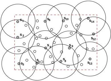
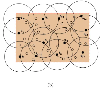
Figure 2.2(a) shows an example sensor network where sensors are deployed ran-domly on a rectangular areaA. E-nodes and N-nodes are illustrated in different formatted circular dots, i.e., E-nodes with dark circles in Figure 2.2(b). Sensing region boundary of an E-node is plotted with dashed-circles. The union of sensing regions covers the entire sensing field. Therefore, by selecting the E-nodes, we guarantee that (i) when an event occurs, it is detected by at least one E-node and (ii) when the sink sends a query to all E-nodes, the query affects the entire sensing field.
(a) An example randomly deployed WSN.
s
s
s
s
2
9
s3 5
6
8
s10
s1 s14
s
s6
s12
s13
(b) Same WSN after classification algorithm.
Figure 2.2: Classification of sensor nodes in ART.
w(i, Ri) =ei·[|Ri|], (2.7)
whereei is the energy level given in (2.1) and [|Ri|] is the area of sensing region Ri.
Then, we calculate thebenefit of selecting each sensor using the weight function. To do this, we first find the size of the area that can be covered by sensor si and has not
been covered yet. Consider the sensorsi with sensing region Ri. Let RC be the area that
sensors of Ccovered so far, i.e.,Ss
j∈CRj. Beneficial area ofsi is defined to be the region inside the sensing field which has not been covered, i.e., RC=Ri∩A)/RC. Hence, benefit
function for sensorsi is the total weight of its beneficial area, which is given as:
benef it(si) =w(i, (Ri∩A)/RC), (2.8)
whereRi is the sensing region of sensorsiand RCis the total region covered by the sensors
inC.
SinceAlgorithm 2.1is to find a near-optimal coverage set, let us take a look how the proposed algorithm approximates an optimal coverage set.
Lemma 1 Algorithm 2.1 gives a coverage set where the total weight of the entire field is
Proof 1 Let τ be the unit area and A be the size of the sensing field in terms of unit τ. Algorithm 2.1 terminates when the sensing area of size A is fully covered. Consider the worst case where all N nodes have the minimum overlapping sensing regions covering the field, then all nodes will be selected as E-nodes.
Let each unit area have apricedefined as follows:
price(τ) ={ei |τ ∈Ri, si∈C}.
Algorithm 2.1attempts to cover the entire field by maximizing the total weight, which is also equal to the summation of the price of each unit area in the sensing field, i.e., PA
j=1price(τj). At thejth iteration, the remaining uncovered area can be covered by a total
weight of at most A−OP Tj+1, where OP T is the total weight of the optimal solution. Then we can write:
Algorithm 2.1Selecting Essential Nodes
Input: S ={s1, s2, s3, . . . , sN} is the set of sensors which are distributed randomly onA.
A sensor hassi = (ri,Ri,ei, (xi, yi)) whereri is sensing range;Ri is sensing
region;ei is residual energy level; and (xi, yi) is location coordinates.
Output: Coverage set,C. I.Initialize
C :=∅
Let RC be total sensing region of C
II.Repeat
Let S−C={s1, s2, . . . , sn}be the candidates,
max benefit := 0; for each si∈S−C
Calculate the energy-benefit of si
benef it(si) := Paj∈(Ri∩A)/RCwi(aj);
if(ebenef it ≥ max benefit)
max benefit :=benef it;
temp:= si;
end if; end for;
C :=C∪temp; Until A⊆RC
s s 2 9 s10 s6 (a) s s s s 2 9 s 5 3 6 8 s10
s1 s14
s
s6
s12
s13
(b)
Figure 2.3: Walking through algorithm 2.1.
PA
j=1price(τj)≤P
A
j=1A−OP Tj+1 =OP T.HA,
where HA is harmonic number. Therefore,Algorithm 2.1 finds an E-node set that covers
the entire field at the cost of O(lnA)-f actor of the optimal solution.
Consider a network with a total number ofN sensors with sensing rangesr. When the sensors are placed such that overlapping sensing areas are minimum, size of sensing field will be at most √27N(r)2/2 under the assumption of full coverage [84]. Thus, the factor of the optimal total weight is obtained as O(ln(N)) for fixed sensing ranges. A loose bound of the running time of Algorithm 2.1 is polynomial with upper bound O(N2).
Finally, in Figure 2.3, we give an example showing howAlgorithm 2.1finds the coverage set. Figure 2.3 (a) shows an intermediate step of the algorithm while Figure 2.3 (b) depicts the final status. In the first step, all nodes are candidates and the coverage set Cis empty. Then, each run of Part II in Algorithm 2.1chooses an unselected node that has the maximum benefit. Figure 2.3 (a) shows the sensing field after the fourth run of Part II. In this example, sensor s9,s6,s2 ands10 are selected based on their benefits and added
to setC. In the next step, uncovered area is A/{R9∪R6∪R2∪R10}. In Figure 2.3 (a),
the next step until the entire sensing field is fully covered as shown in Figure 2.3(b).
2.3.2 Coverage Set Update
The second challenge is how to update the coverage set. E-nodes should be updated throughout the lifetime of the WSN for two reasons: (i) to handle the unexpected E-node failures, (ii) to acquire fairly distributed energy consumption among sensors.
In general, there are two methods to updating the coverage set. The first method is called global update where all E-nodes are re-selected independent from the current set. In particular, global update is the process of repeating classification algorithm with latest residual energy levels of sensors. By this way, sensors that have overlapping regions and was E-Nodes in the previous round might be an N-node in the next update because more energy has been consumed when they were E-node before. This is used to acquire fairly distributed energy consumption among sensors. However, such a global maintenance may incur high overhead if repeated in short periods and can not handle the unexpected E-node failures during an update interval.
The second method is on-demand local update which can handle E-node failures immediately. Local update is triggered when an unexpected E-node failure is detected by the sink. In this case, N-nodes covering the sensing region of failed E-node are assigned to be an E-Node by the sink. It may not be possible to find one N-node instead of failed E-node; however, it is much efficient instead of global update in any E-node failure.
In ART, we combine local and global such that, in case of an node failure new E-nodes are selected locally where global update will be performed for longer predetermined update intervals. Sink can monitor up-to-date energy reserves of sensors using a energy monitoring scheme [82]. Based on this remaining energy of sensors, a new essential set is formed by runningAlgorithm 2.1. After each global update, sink informs sensors of their type by using a control message. The effects of update interval on network lifetime and energy consumption is discussed in Section 2.5.
with node coordinate information need to be disseminated within the network towards a single node (e.g., sink node). In [1], it is shown that collecting information from a sink node is more power-efficient manner compared to spreading this information to each and every other node within the network. In addition, choosing the sink node as the target of data propagation is reasonable if we considers that the sink node has ample energy and com-puting power compared to individual sensor nodes. Having the global view of the network at the sink node provisions algorithms for closer-to-optimal coverage set determination as well.
Finally, using a centralized scheme can relieve processing load from the sensors in the field and help in extending the overall network lifetime by reducing energy consumption at individual nodes. The proposed greedy algorithm runs on the sink with an approximation ratio of lnN, providing very close-to-optimal coverage sets for most instances of the sensor deployments. Additionally, maintaining the node set selections (i.e., E-node updates) can be realized through low cost information diffusion methods.
2.4
ART Protocol Operations
ART is an asymmetric and reliable transport mechanism which provides end-to-end reliability in two directions based on energy-aware node classification and a congestion control mechanism. In this section, we describe the details of ART protocol operations, which includes three main functions:
1. Reliable query transfer 2. Reliable event transfer
3. Distributed congestion control
temporarily squelching the traffic of N-nodes. Note that, when there is no congestion, both E-nodes and N-nodes participate in relaying messages to the sink. However, only E-nodes are responsible in providing end-to-end event and query reliability by recovering the lost messages.
2.4.1 Reliable Query Transfer
Reliable query (sink-to-sensors) transfer is provided using negative acknowledg-ments sent from E-Nodes to the sink if there is a query loss. Since the queries sent by the sink are in order, sensors can detect the lost message by use of sequence numbers in the query messages. An NACK message is sent if a gap is detected, i.e., an out of sequence number, when sink sends a new query message to the E-Nodes. When an E-Node detects a gap in the sequence number of the new query, it sends an NACK back to the sink to recover the previous query. This procedure is described inAlgorithm 2.2.
However, lost query messages can be detected when E-Nodes receive a new query message. This may result in two problems. First, loss of the last query message can not be detected. Consider the last message qk with sequence number k is lost. E-Node may not
handle the lost message since there is no consecutive query. Second, the query transmission frequency might be very low such that lost queries can not be recovered before timeout. To differentiate the final query message, we use an extra Poll/Final (P/F) bit which can be set by the sink node. P/F bit is set either when a message is the last query or the next query will not be sent before timeout. And the sink retransmits this message until an ACK is received because ACK mechanism is used in reliable event transfer. Therefore, E-Nodes which receive a query with P/F bit set send an ACK to the sink, indicating the query is received successfully.
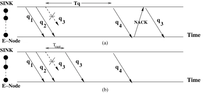
An example query transmission scenario is illustrated in Figure 2.4. In Figure 2.4 (a), the P/F bit is not used. When the sink sends queries 1, 2 and 3 consecutively where query 3 is lost. After query 3, the sink decreases the query transmission frequency and sends q4 after a time period Tq. In this case, q3 is recovered when q4 is received. If loss
recovery period (i.e.,Tq) is very long, even thoughq3can be recovered, long recovery period
Algorithm 2.2Reliable Query Transfer
Input: Given a sensor network G; Sink has a set of queries Q = [q1, . . . , qk, qk+1, . . .].
1. Sink: Send the in-sequence queries with sequence numbers 1,2,..k.
2. E-Node: Receive the messages for qk. Check the sequence number for loss detection.
3. E-Node: If a gap is detected in the sequence numbers, send an NACK to recover the lost message.
4. Sink: Retransmit qk−1 if a NACK is received.
5. E-Node: When the queries are successfully received, check P/F bit. If P/F bit is set, send an ACK to the sink. (details in Section 2.4.3)
Sink: Retransmits the message with P/F bit is set until the ACK is received.
at the sink. This method is very helpful when the query traffic pattern is not uniformly distributed in which case, the interarrival time between queries are not constant. Then the use of P/F bit makes the transport protocol flexible and reliable.
Tq q q 1 2 q 3 q 4 q 3 (a) NACK q q 1 2 q 3 q 4 q 3 (b) Time Time SINK E−Node SINK Tout E−Node
Figure 2.4: Example of query loss.
2.4.2 Reliable Event Transfer
each message may result inefficient use of battery power, which is considered to be a very scarce resource in WSNs.
For event reliability, we propose alightly-loaded ACK mechanism between the E-Nodes and the sink node given inAlgorithm 2.3. Each E-Node waits for acknowledgment for only the first message that reports an event, i.e., event-alarm. When a new sensing value is obtained, an E-Node decides if it reports an event or not. If it is anevent-alarm, it simply marks the message by setting theEvent Notification (EN) bit. Therefore, the sink node sends ACK for the only messages which are marked as event-alarm. EN bit, is used to force the sink to send acknowledgment. Event-alarm rate depends on the distribution of events detected in the sensing field. Similar to downstream communications, only the E-Nodes are responsible for waiting the acknowledgment and may retransmit if necessary.
As an example, in Figure 2.5 an event transfer scenario is illustrated wherev3 and v6 are event-alarm messages and their EN bits are set. In this example, the first event
alarm message is received by the sink, and the ACK is transmitted. However, next alarm message v6 is lost. Since the sender is responsible for loss detection and recovery, E-Node
retransmits v6 after retransmission timeouts shown in Figure 2.5. Therefore, loss recovery
is triggered only for event-alarm messages by the E-Node, which is very effective in energy saving as shown in Section 2.5.
2.4.3 Distributed Congestion Control
Given a WSN consisting of large number of nodes, congestion is an inevitable problem because a large number of sensors may transmit the sensed event at the same time. To detect and avoid congestion, several works has been proposed using different mechanisms in WSNs [33, 56, 79]. In [56], congestion is detected by monitoring the buffers
Algorithm 2.3Reliable Event Transfer Input: Given a sensor network G;
An E-Node is sending an event-alarm vkEA given timeouttout;
1. E-Node: Ifvk=vkEA, set the EN bit, send to the sink, then start timer and buffer vkEA
until an ACK is received.
Otherwise, send it to the sink, delete from the buffer. 2. Sink: Send an ACK if it receives a vEAk
d d d
d d d d d
d
ACK
2
1 3 4 5
6
6
7 8
SINK
Time
Tout
E−Node
Figure 2.5: Example of event-alarm loss.
of sensor nodes. When congestion is detected, sensors inform the sink node to decrease the reporting frequency of the network. A different method is that congestion detection is based on local channel monitoring and the congestion is propagated through hop-by-hop back-pressure messages upstream toward the source [79].
Unlike these existing solutions, in ART, congestion control is handled by the E-nodes in a distributed manner. It is based on monitoring the ACK packets of event reports. If an ACK is not received during a timeout period by the E-node, traffic of non-essential sensors is reduced by sending them congestion alarm messages, which will temporarily make them stop sending their measurements. When an ACK is received, congestion-safe message is announced to resume normal operation of the network.
It is possible that lost data packets may not indicate an accurate congestion for WSN because losses can be caused by link failures or congestion [68]. However, in ART we monitor only the event-alarm messages which report the sensed events. Congestion often occurs when events are reported by several sensors [79]. When an event is detected, many correlated event messages are sent to the sink, especially if the event is sensed in a large area and the network is dense, e.g., earthquake detection. Thus, monitoring the loss event-alarm messages is an efficient and simple way to detect congestion. Another advantage of this mechanism is its ease of use, since we already use a timer for retransmission of event-alarms. Thus, congestion timeout can be determined in accordance with retransmission timeout, which will be explained in Section 2.4.4. Each E-node decides and triggers the congestion control procedure without the centralized control of sink, based on receiving the ACK of an event-alarm.
temporar-ilypassive via congestion alarm messages. Being passive for a sensor here means not sending sensing measurements to the sink. First, an E-node, which detects a congestion, will broad-cast a congestion alarm (CA) message. After timeout period, if the congestion is still not relieved, an E-node will resend the CA by increasing thehop-count. This will continue until the congestion is relieved. From the N-nodes point of view, when they receive a CA message, they temporarily stop sending their sensing measurements and decrease the hop-count. The CA message is flooded until the hop-count is 0.
Note that N-nodes may receive multiple CA messages,CA= [CA1, CA2, ..], which are sent by an E-node sequentially until the congestion is relieved. EachCAj includes hop-count denoted by hop-count(j) = j. Because E-Nodes increase hop-count in every CA message, CA messages are flooded up to j-th neighbors of the E-node. When the ACK of an event is received, E-node sendscongestion safe (CS) message similar the CA to resume the normal operation of the network. Congestion safe message is sent with the hop-count value of the latest CA message by the E-node. Therefore, the number of sensors sending their measurements is reduced, thus regulating the excessive traffic for congestion control.
2.4.4 Timeout and Retransmissions
In ART, we use an asymmetric protocol, e.g., NACK for sink-to-sensor and ACK for sensor-to-sink communication. While using NACKs, the sink only retransmits if it receives an NACK for a query message. Therefore, no timer is used. However, while transferring events from sensors to the sink, E-nodes wait ACKs for event-alarm messages. When an E-node sends an event alarm message, it triggers the timer and waits fortimeout period to detect congestion or retransmit. Thus, timeout periods becomes particularly important and will be discussed in this section.
ART uses timeouts for both reliable end-to-end delivery and congestion control. We use congestion timeout (CTO) for congestion detection, which is dynamically deter-mined based onround trip time (RTT) similar to adaptive retransmission timeout in TCP. Assume that all sensors have an initialRT T that is the duration between the time when a message is sent and the time when the ACK of the message is received at the sender. Then,
CA sent
t0 t0+ RTT t1
sent CA(2)
CTO
t3 sent CA(3)
t
(1)
v(k) event−alarm
sent
retransmit
v(k) v(k)retransmit v(k)retransmit
t1+T∆t t2 t2+T∆t t3+T∆t
CTO CTO
Figure 2.6: Retransmission and congestion control behavior.
Thus, E-nodes can determine the RT T(sample) by comparing the time stamp received by ACK. Then, the estimated RTT is determined by exponential averaging as:
RT T(t) =α∗RT T(t−1) + (1−α)∗RT T(sample)
CT O(t) =η∗RT T(t),
whereα∈(0,1) is weight ratio, and η >1 indicates the coefficient of delay tolerance of the application.
Retransmission is done after eachretransmission timeout (RTO) when necessary. However in ART, we let RTO equal to CTO used for congestion detection. CA messages are sent when the timer expires. Clearly, it is not efficient to retransmit and send the CA message at the same time. Hence
RT O(t) =CT O(t) +ξ, (2.9)
where ξ is the one-hop transmission delay. Event alarm messages are retransmitted after
ξ of sending the CA message. Note that, different from other wireless and wired transport protocols, retransmission does not block the next data transmissions in WSNs. We continue sending next messages and retransmit the lost message if needed. The detailed time diagram of retransmission and congestion control in ART is shown in Figure 2.6 in which t is the time instant.
• t=t0: Suppose an E-node detects an event at timet0 and immediately reports it by
• t=t1: At timet1, CTO timer expires. As shown in Figure 2.6,CT O is greater than
the estimated RTT. When the timer expires, the first congestion alarm message is sent by the E-node. The N-nodes which receive theCA(1) do not send their measurements until they receive a congestion safe message.
• t=t1+T∆t: According to Algorithm 2.2, E-node waits until t=t1+T∆t. Then,
it retransmits the event-alarm. By retransmissions, the CTO timer is restarted.
• t = t2: During t = t1 +T∆t to t = t2, the E-node continues waiting for the ACK.
At time t2, since CTO timer expires, CA(2) is sent by increasing the hop-count.
Until receiving an ACK from the sink, retransmission and CA steps will be repeated consecutively similar ast=t1 andt=t1+T∆t.
In ART, only the first message with an event information needs to be acknowledged and retransmitted if necessary. Since this message has a setting bit EN bit, the sink will send an ACK for this message. In other words, event information is guaranteed to reach the sink node, whereas not every message is guaranteed, which is to achieve the objective of event reliability. Therefore, the number of retransmissions is decreased which in turn will reduce the energy consumption.
2.5
Performance Evaluation
The proposed ART protocol is implemented in the ns-2 [47] network simulator. We conducted several simulations using different scenarios in a static sensor network. The performance of ART is evaluated regarding the effectiveness of classification algorithm, energy balance, network lifetime, and node density.
2.5.1 Performance Metrics and Simulation Setup
We use the following metrics to characterize the performance:
• Network lifetime: It represents the maximum time interval that a network can main-tain its functionality. We consider a WSN as alive when every point in A is covered by at least one sensor.
• End-to-end delay: It is the time for a packet to arrive at transport entity of the receiver after transmitted by the transport entity of the sender.
• Packet loss ratio: It is the ratio of the number of packets lost to the number of packets generated.
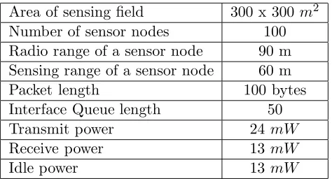
Simulations are performed for randomly placed sensor nodes in a rectangular re-gion. All sensor nodes have a sensing region of fixed range, r, associated with them. A communication edge exists between two sensors nodes if they are within their transmission range. A sensing field of 300 x 300m2 is used in simulations. We vary the number of sensors
which allows us to study the performance from very sparse to very dense networks. The number of sensors should be sufficient to cover the sensing field for given parameters. Note that only the density of sensors affects the performance of the node classification algorithm, thus there is no need to vary the size of the area.
In the basic scenario, 100 fixed sensor nodes having transmission range of 90 m and sensing ranges of 60 m are used. We use the energy model given in Section 2.2.2 where initial energy of sensors are 3 J.
Before we describe the performance results, we explain the application run on sensors and the sink. In the experiments, we use a mobile tracking application in which the movements of mobile nodes are reported to a sink. Mobility pattern of a mobile (phe-nomenon) node is generated using Gauss-Markov mobility model [77] at a maximum speed of 20 m/sec. An event is defined to detect the phenomenon node in the sensing area of a sensor.
Table 2.2: ART simulation parameters. Area of sensing field 300 x 300 m2
Number of sensor nodes 100 Radio range of a sensor node 90 m Sensing range of a sensor node 60 m
Packet length 100 bytes
Interface Queue length 50
Transmit power 24 mW
Receive power 13 mW
Idle power 13 mW
a continuous data delivery model, by sending periodic queries to the sensors. Similarly, we use query-reporting frequency, as a simulation parameter to maintain traffic load in downstream direction. Queries sent by the sink do not affect the scenario or sensing period in the simulation. The coordinates of the sink is the center of the sensing field and same for all experiments. CSMA/CA is used as the MAC protocol and AODV is used as the routing protocol [53].
2.5.2 Simulation Results
We start by illustrating the effectiveness of the energy-aware node classification algorithm (Algorithm 2.1), i.e., the size of coverage set for various network densities. We then discuss the effect of update interval, which is an important question to find the value of update interval for a given sensor network. We then show the effect of update interval on network lifetime. Further, performance gains of reliable event and query transfer service are shown over message-level reliable service. These gains demonstrate the unnecessary overhead that is generated when message-level reliability is concerned instead of event and query reliability which is guaranteed by persisted retransmissions for all experiments.
0 20 40 60 80 100 150 140 130 120 110 100 90 80 70 60 50 40 30 20 10 0
E-Node Ratios (%)
Time(sec) E-Node Ratios (%) over Time
N=100 N=150 N=200
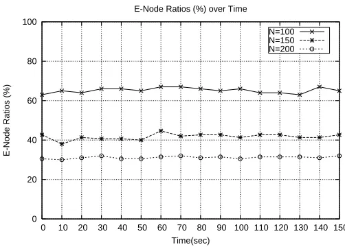
Figure 2.7: E-Node ratio of coverage set vs. network density (T∆U = 10 sec).
to find coverage sets regardless network density with a decreasing E-node ratio as the network density increases. Therefore, the weighted-greed algorithm for node classification is even more effective in reducing the cost of reliability in dense networks. Further, results in Figure 2.7 indicate that the ratio of E-nodes does not vary in time. In every 10 seconds, our algorithm finds a new coverage set which is independent from the previous set. This implies that no matter what changes occurred in an update interval, E-nodes can always be selected.
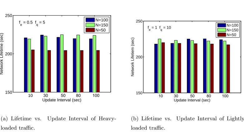
Effect of Update Interval on Lifetime. For performance evaluation of ART protocol, selecting a proper time interval is very important for a given network. A very large value may increase the communication cost, thus reducing residual energy. On the other hand, a very small update interval may cause high variance in sensors residual energy as E-nodes may drain out their battery much faster, thus partitioning the network. Thus, we study the effect of update interval on network lifetime.
sce-10 30 50 80 100
150 200 250
Update Interval (sec)
Network Lifetime (sec)
N=100 N=150 N=50 f
e = 0.5 fq = 5
(a) Lifetime vs. Update Interval of
Heavy-loaded traffic.
10 30 50 80 100
150 200 250
Update Interval (sec)
Network Lifetiem (sec)
N=100 N=150 N=50 fe = 1 fq = 10
(b) Lifetime vs. Update Interval of
Lightly-loaded traffic.
Figure 2.8: Effect of update interval on network lifetime.
nario in Figure 2.8 (a). Before and after 30, lifetime curve follows a non-decreasing and non-increasing trend, respectively. We observe the same trend in lightly loaded scenario of network with 100 nodes in Figure 2.8 (b). However, this time the peak value is 80 sec. This signifies that scenario with lightly-loaded traffic has longer update interval than the heavy traffic network.
In this experiment, we also present the performance of networks having different packet load. We generate different packet loads by varying the event-reporting (fe) and
query-reporting frequency (fq) parameters. In Figure 2.8, two different packet loads are
performed: (i) heavy: fe= 0.5 andfq = 5 and (ii) light: fe= 1 and fq= 10 sec.
0 0.5 1 1.5 2 2.5 3 3.5 4
100 200 300 400 500
End-to-End Delay
Node Density TTS fe=0.5
TTS fe=5 alwaysActive fe=0.5
(a) Effect of query/event reliability on E2E delay.
0 0.2 0.4 0.6 0.8 1
50 100 150 200
Packet Loss Ratio
Node Density ART fe=0.1 fq=2
MLR fe=0.1 fq=2 ART fe=0.5 fq=5 MLR fe=0.5 fq=5 ART fe=1 fq=10 MLR fe=1 fq=10
(b) Effect of query/event reliability on packet loss.
MLRfor various network densities and packet loads. Initial roundtrip time (RT T = 2 sec), coefficient of adaptive RTT (α = 0.125), coefficient of delay tolerance (η= 0.8) and one-hop transmission delay (ξ= 0.05 sec) are used as input parameters.
Figure 2.9 compares the performance of ART and MLR with respect to average end-to-end delay and packet loss ratio. We have simulated three types of traffic load scenar-ios: (i) heavy: fe= 0.1 andfq= 2 and (ii)moderate: fe= 0.5 and fq= 5 (iii) light: fe = 1
and fq = 10 sec. From Figure 2.9 (a), we find that the end-to-end delay is a function of
increasing network density. Notice that under all traffic loads, end-to-end delay of ART is 40% lower than MLR on average. The reasons for reduced delay are twofold: the advantage gained by having classified E-Nodes dealing with retransmissions reduces the amount of data sent, and the advantage gained by using event-based reliability to avoid ACK implo-sion. Also, end-to-end delay in ART degrades gracefully with decrease in traffic load. Even in heavy packet load, the delay in ART protocol remains below 5 sec. The packet loss ratio is shown in Figure 2.9 (b) where even at heavy load, ART yields less packet losses than MLR scheme.
0 2 4 6 8 10 12 14
50 100 150 200
End-to-End Delay
Node Density ART fe=0.1 fq=2
ART-noCC fe=0.1 fq=2
ART fe=0.5 fq=5
ART-noCC fe=0.5 fq=5
ART fe=1 fq=10
ART-noCC fe=1 fq=10
(a) Effect of congestion control on E2E delay.
0 0.2 0.4 0.6 0.8 1
50 100 150 200
Packet Loss Ratio
Node Density ART fe=0.1 fq=2
ART-noCC fe=0.1 fq=2 ART fe=0.5 fq=5 ART-noCC fe=0.5 fq=5 ART fe=1 fq=10 ART-noCC fe=1 fq=10
(b) Effect of congestion control on packet loss.