Development of Instrumental Techniques for Color Quality Control of Complex Colored Pattern.

(1)

CAO, RENBO. Development of Instrumental Techniques for Color Quality Control of Complex Colored Patterns. (Under the direction of Dr. Renzo Shamey.)

Marine Pattern (MARPAT) is a type of camouflage pattern used in the United States Marine Corps.

At present Pass/Fail assessment of the reproduced camouflage samples is performed subjectively by a few

experts under controlled conditions following specific procedures. However, there are lots of factors that

can affect the accuracy and precision of the assessment. Hence, a digital camera based imaging system

was developed to carry out Pass/Fail judgment of MARPAT camouflage samples. To achieve this goal,

three main tasks were performed.

The first task was to conduct a psychophysical experiment to establish Pass/Fail boundaries of

MARPAT samples by employing 4 expert observers who assessed 110 samples. Each observer repeated

the experiment three times. Intra- and inter-observer variability was analyzed. It was found that the

overall agreement between observers was less than 50%. MARPAT samples failed due to not only color

defects but also other appearance defects. Observers gave Fail responses mainly to Green and Coyote

colors, which are dominant colors of MARPAT pattern. The Pass/Fail threshold based on CIEDE2000

color difference using a psychophysical function is 2.2 and 1.9 for Green and Coyote, respectively.

The second task was to investigate the effect of noise on digital camera based colorimetry. Spatial

and temporal noise models were developed for five commercial cameras. Error propagation method

was employed to evaluate the effect of noises in the CIELAB color space. Ellipsoids at 95% confidence

level were obtained. Temporal noise was found to be significantly larger than spatial noise. Size of

ellipsoids of both noises exceed that of unit CIEDE2000 ellipsoid, which is approximately the threshold

of acceptability of solid color reproduction.

The last task was to calibrate a digital camera and perform Pass/Fail judgments using the developed

system. Color gamut of camouflage colors is limited compared with that of commercial color checkers

and accuracy of color correction using these color charts is not satisfactory considering low Pass/Fail

(2)

The mean, maximum and standard deviation of color conversion error (CIEDE2000) are approximately

0.41, 1.17 and 0.2 for 444 colors, respectively.

The developed imaging system is faster than a spectrophotometer, and is more consistent than

(3)

(4)

by Renbo Cao

A dissertation submitted to the Graduate Faculty of North Carolina State University

in partial fulfillment of the requirements for the Degree of

Doctor of Philosophy

Fiber and Polymer Science

Raleigh, North Carolina

2016

APPROVED BY:

Dr. Renzo Shamey Chair of Advisory Committee

Dr. H. Joel Trussell

(5)

To the loving memory of my grandfather.

To my parents, my sister, my grandmother and my girlfriend, who have stood behind me and supported

(6)

Renbo Cao comes from Xuanen, Hubei province, China. He received his Bachelor’s and Master’s degree

from Wuhan University and South China University of Technology, China, in 2008 and 2011 respectively.

In August 2011, he came to NC State to pursue a Ph.D. in color science. His interests cover fundamental

(7)

I would like to thank Dr. Renzo Shamey for first of all agreeing to be my advisor, and then his advice,

support, patience and guidance throughout this research.

I would like to thank Dr. H. Joel Trussell for sharing his knowledge in the field of digital image processing

and providing constructive comments as well as helping me to develop my mathematical skills .

I am thankful for Dr. Brand Fortner and Dr. Christopher G. Healey for their useful insights into making

this dissertation a reality.

I am thankful to all observers participated in various psychophysical experiments in the past four and

half years.

I am very grateful for the help received from Dr.Yu Lin in the preparation of this dissertation and valuable

suggestions in the research.

I am thankful for Cheng Chen and Han Jiang for providing Canon cameras used in the noise estimation

experiment.

Also thanks are due to the former and current group members: Dr. Gang Fang, Dr. Eunjou Yi, Dr.

Yuzheng Lu, Dr. Juan Lin, Dr. Weethima Sawatwarahul, Dr. Kiarash Arangdad, Mr. Charles Stewart, Mr.

Muhammad Zubair, Mr. Sajeesh kumar Kulappurath and Ms. Sonali Mandal.

Finally, I would like to thank my friends: Kun Fu, Nanshan Zhang, Xiaohang Sun, Yongxin Wang,

(8)

LIST OF TABLES . . . viii

LIST OF FIGURES . . . ix

Chapter 1 INTRODUCTION . . . 1

1.1 Problem Statement . . . 1

1.2 Dissertation Overview . . . 2

Chapter 2 Literature Review . . . 3

2.1 Human Color Vision . . . 3

2.1.1 Physiology of Human Color Vision . . . 4

2.1.2 Human Color Vision Theory . . . 11

2.2 Psychophysics in Color Science . . . 14

2.2.1 Threshold Experiments . . . 14

2.2.2 Matching Experiments . . . 16

2.2.3 Scaling Experiments . . . 16

2.2.4 Design of Psychophysical Experiments . . . 17

2.3 Colorimetry . . . 18

2.3.1 Basic Colorimetry . . . 18

2.3.2 Advanced Colorimetry . . . 25

2.4 Digital Still Camera Based Colorimetry . . . 29

2.4.1 Digital Camera Architecture and Pipeline . . . 30

2.4.2 Digital Camera Noise . . . 30

2.4.3 Digital Camera Color Calibration . . . 33

2.5 Conclusions . . . 46

Chapter 3 MARPAT Sample Analysis . . . 47

3.1 Overview . . . 47

3.2 MARPAT Camouflage Samples . . . 47

3.3 Methods . . . 49

3.3.1 Measurement of MARPAT Samples . . . 49

3.3.2 Variability Analysis Methods . . . 49

3.4 Results and Discussions . . . 50

3.4.1 Spectrophotometer Variability . . . 50

3.4.2 Intra-sample Variability . . . 52

Chapter 4 Establishment of PASS/FAIL Boundaries . . . 58

4.1 Introduction . . . 58

4.2 Method . . . 60

4.2.1 Psychophysical Experiment . . . 60

(9)

4.3.2 Establishment of Pass/Fail Boundaries . . . 73

Chapter 5 Digital Camera Noise Analysis . . . 116

5.2 Method . . . 118

5.2.1 Experimental Design . . . 119

5.2.2 Experimental Protocol . . . 121

5.2.3 Error Propogation Method . . . 123

5.3.1 Linearity of Camera Response . . . 125

5.3.2 Spatial Non-uniformity Analysis . . . 126

5.3.3 Noise Modeling . . . 129

5.3.4 Effect of Noise on Digital Camera Based Colorimetry . . . 136

Chapter 6 Digital Camera Calibration . . . .147

6.2 Method . . . 149

6.2.1 Experimental Design . . . 149

6.2.2 Segmentation of MARPAT Images . . . 153

6.2.3 Digital Camera Calibration Methods . . . 156

6.3.1 Camera Calibration Using CCDT and CCSG . . . 158

6.3.2 New Color Calibration Chart . . . 164

Chapter 7 Digital Camera PASS/FAIL Judgment . . . 172

7.1 Overview . . . 172

7.2 Intra-Sample Variability . . . 173

7.2.1 Analysis Procedure . . . 173

7.2.2 Results and Discussions . . . 173

7.3 Pass/Fail Judgment . . . 175

Chapter 8 Conclusions and Future Works . . . 182

8.2 Future Works . . . 184

BIBLIOGRAPHY . . . 188

APPENDICES . . . 205

(10)

A.3 Pass/Fail Terminology . . . 207

Appendix B Propagation of Noise . . . 211

B.1 Covariance of Noise in RGB Space . . . 211

B.2 Covariance of Noise in CIEXYZ Space . . . 212

(11)

Table 2.1 Classification of Scale Types. . . 18

Table 2.2 Classification of Digital Camera Noise. . . 32

Table 2.3 The polynomial regression coefficients . . . 37

Table 4.1 2×2 contingency table for two observers’ responses. . . 65

Table 4.2 Coefficient of fitted linear functions and the predicted color difference values for Pass/Fail boundary based on 75% and 50% agreement with current visual FAIL responses. . . 103

Table 4.3 Statistics of color difference between 110 samples and the standard. . . 104

Table 4.4 Percentage of pass and fail samples due to individual color that observer agreed in three trials. . . 104

Table 4.5 Number of observers’ contradictory comments for samples in three trails. . . 106

Table 4.6 The number of pass and fail samples based on the prediction of two methods. . . 108

Table 4.7 Color differences between colors under two illuminants with and without chro-matic adaptation. . . 113

Table 4.8 Coefficients of fitted linear functions and the predicted color difference values based on 75% and 50% agreement for FAIL responses. . . 114

Table 4.9 The number of pass and fail samples based on the predictions of two methods under IllDigiEye. . . 115

Table 5.1 Digital camera parameters and settings. . . 120

Table 5.2 The estimated coefficients of PRNU noise model for each camera. . . 129

Table 5.3 The estimated coefficients of temporal noise model for each camera. . . 136

Table 5.4 The length of the semi-axes of spatial and temporal noise ellipsoids of the yellow color center and the radius of the sphere with an equal volume to that of the ellipsoid.141 Table 6.1 The polynomial regression coefficients. . . 158

Table 6.2 Training and testing results (CIEDE2000) using CCSG color checker . . . 159

Table 6.3 Traing and testing results (CIEDE2000) using the CCDT color checker. . . 164

Table 6.4 Calibration results of all MARPAT colors using selected training data via different selection methods (MSE cost function). . . 167

Table 6.5 Calibration results of all MARPAT colors using selected training data via different selection methods (CIEDE2000 cost function). . . 168

Table 6.6 Training and testing results (CIEDE2000) using the new MARPAT color char. . 168

Table 6.7 Training and testing results (CIEDE2000) using the new MARPAT color chart. . 170

Table 7.1 The number of pass and fail samples based on the prediction of two methods. . . 178

Table 8.1 Summaries of the Pass/Fail judgement using difference methods. . . 184

(12)

Figure 2.1 The primary visual pathway. . . 5

Figure 2.2 Schematic diagram of the human eye. . . 6

Figure 2.3 Structure of primate retina. . . 7

Figure 2.4 Distribution of rods and cones cells in human retina. . . 8

Figure 2.5 Structure of LGN cells. . . 9

Figure 2.6 Human visual corte. . . 10

Figure 2.7 Visual stream from retina to visual cortex. . . 11

Figure 2.8 Visual stream from retina to visual cortex. . . 12

Figure 2.9 Schematic illustration of two-stage color theory. . . 13

Figure 2.10 Schematic illustration of three-stage color theory. . . 15

Figure 2.11 Schematic illustration of color matching experiment. . . 19

Figure 2.12 Procedure for deriving cone fundamentals as a function of field size. . . 21

Figure 2.13 Specification of components of the viewing field. . . 26

Figure 2.14 Schematic diagram of the CIECAM02 computation process. . . 29

Figure 2.15 Block diagram of the hardware components used in a typical digital camera. . . . 31

Figure 2.16 Overview of the ICC color management architecture. . . 35

Figure 2.17 Illustration of Trilinear interpolation. . . 39

Figure 2.18 Typical Architecture of an MLP Neural Network. . . 41

Figure 3.1 One repeat unit of MARPAT camouflage pattern . . . 48

Figure 3.2 Spectral power distribution (SPD) of the light sources. . . 50

Figure 3.3 Reflectance of BCRA tiles. . . 51

Figure 3.4 Spectrophotometric variability determined using BCRA tiles. . . 52

Figure 3.5 Intra-sample variability of 112 samples. . . 53

Figure 3.6 Histogram plot of the mean and maximum color difference and coefficient of variation (CV) of individual samples for SPIN and SPEX mode usingMethod 1. 54 Figure 3.7 Histogram plot of the mean and maximum color difference and coefficient of variation (CV) of individual samples for SPIN and SPEX mode usingMethod 2. 55 Figure 3.8 Intra-sample variability in terms of component differences of 112 samples. . . 56

Figure 3.9 Intra-Sample variability in terms of component differences of 112 samples. . . . 57

Figure 4.1 MARPAT camouflage samples including those selected (in red) for the psy-chophysical experiment. . . 60

Figure 4.2 MARPAT camouflage samples including those selected (in red) for the psy-chophysical experiment. . . 61

Figure 4.3 Illuminanting and viewing geometry of MARPAT samples used in visual evaluation. 63 Figure 4.4 Relationship between|φ|andχ2. . . 66

Figure 4.5 Intra-observer variability based onW D. . . 70

Figure 4.6 Intra-observer variability based onφ(ID VS. ID). . . 70

Figure 4.7 Intra-observer variability based onφ(ID VS. Mean). . . 71

(13)

Figure 4.10 Percentage of pass samples based on each color and the overall visual results. . 74 Figure 4.11 Distribution of pass and fail samples in the CIELAB color space. . . 74 Figure 4.12 Z-score and accumulative probability of standard norm distribution. . . 75 Figure 4.13 Total number of times each term was used by the four experts in three repetitive

trials for the 110 samples. . . 77 Figure 4.14 Reationship between the number of samples and proportion of responses of other

appearance defects. . . 78 Figure 4.15 Maximum Z-score value of other appearance defects for each sample and the

intra-sample variability of that sample in terms of CIEDE2000 calculated using the mean value of ID VS ID method. . . 79 Figure 4.16 Plot of colorimetric values for Khaki including the standard and unit CIEDE2000

ellipsoid. . . 80 Figure 4.17 Z-score value of responses for Khaki color failure and CIEDE2000 color

differ-ence values. . . 80 Figure 4.18 Percentage of the size of each color in one repeat MARPAT pattern. . . 82 Figure 4.19 The relationship between color difference of Khaki and that of other three color. 82 Figure 4.20 The number of times each term was used for color appearance evaluation of

Khaki color. . . 83 Figure 4.21 Z-score of responses of each term and component color difference for Khaki. . 84 Figure 4.22 Z-score values and color difference values of Khaki color. . . 86 Figure 4.23 Plot of colorimetric values for the Green color including the standard and unit

CIEDE2000 ellipsoid. . . 87 Figure 4.24 The Z-score value of responses for the Green color fail samples and the CIEDE2000

color difference values . . . 87 Figure 4.25 The relationship between color difference for Green colors and that of other three

colors. . . 88 Figure 4.26 The number of times each term was used for the color appearance evaluation of

Green colors. . . 89 Figure 4.27 The Z-score of responses for each term and the component color difference for

Green. . . 90 Figure 4.28 Z-score values and color difference values for Green color. . . 92 Figure 4.29 Plot of colorimetric values of Coyote colors including the standard and unit

CIEDE2000 ellipsoid. . . 93 Figure 4.30 Z-score value of responses for Coyote color fail rarings and the CIEDE2000

color difference values. . . 93 Figure 4.31 Relationship of color difference of Coyote and that of other three colors. . . 94 Figure 4.32 The number of times each term was used for the color appearance evaluation of

Coyote color. . . 95 Figure 4.33 The Z-score of responses for each term and the component color difference for

(14)

Figure 4.36 Z-score values and color difference values. . . 99

Figure 4.37 The number of times each term was used for the color appearance evaluation of Black color. . . 100

Figure 4.38 Z-score value of responses for the Black color fail ratings and the CIEDE2000 color difference values. . . 100

Figure 4.39 Fitted curve for different data. . . 102

Figure 4.40 Percentage of samples that received pass or fail rating from an observer(s) in three trials. . . 105

Figure 4.41 Distribution of data and their visual results in terms of proportion of FAIL ratings from two observers in location 1. . . 107

Figure 4.42 Convex hull, CIEDE2000 ellipsoid of Green and Coyote. . . 109

Figure 4.43 Color shifts from IllDLA to IllDigiEye without chromatic adaptation. . . 111

Figure 4.44 Color shifts from IllDLA to IllDigiEye with chromatic adaptation. . . 112

Figure 4.45 Color differences between samples and the standard under IllDLA and IllDigiEye.113 Figure 4.46 Fitted curve for different data under IllDigiEye. . . 114

Figure 5.1 Imaging system including ColorChecker. . . 119

Figure 5.2 Flowchart of the camera noise evaluation and its effect on colorimetric values experiment. . . 121

Figure 5.3 Flowchart for noise evaluation. . . 122

Figure 5.4 Linearity of the five cameras. . . 127

Figure 5.5 Spatial non-uniformity of five cameras. . . 128

Figure 5.6 Spatial noise estimated from dark images. . . 131

Figure 5.7 Spatial noise estimated based on CCSG images. . . 132

Figure 5.8 Temporal noise estimated based on CCSG images. . . 134

Figure 5.9 Temporal noise estimated based on CCSG images. . . 135

Figure 5.10 Mean ratio of temporal noise to spatial noise of 140 color patches. . . 137

Figure 5.11 Distribution of the difference of pixel values minus the mean value for the green channel. . . 137

Figure 5.12 Noise ellipsoids of a color center. . . 139

Figure 5.13 Noise ellipses of a color center. . . 140

Figure 5.14 The derivative of the cube root function. . . 142

Figure 5.15 Spatial noise ellipsoids of colors of CCSG. . . 143

Figure 5.16 Temporal noise ellipsoids of colors of CCSG. . . 144

Figure 5.17 Relationship between size of noise ellipsoids and Lightness, Chroma and Hue angle. . . 145

Figure 6.1 Color gamut of two color checkers and MARPART samples. . . 150

Figure 6.2 Distribution of colors of CCDT, CCSG and MARPAT samples in the CIELAB color space. . . 151

(15)

Figure 6.5 Standard MARPAT sample and segmentated image as well as the histrogram

plots of the Euclidean norm of RGB values in each cluster. . . 155

Figure 6.6 Best training and testing results using the MSE cost functions. . . 160

Figure 6.7 Best training and testing results using the CIEDE2000 cost functions. . . 161

Figure 6.8 Best training and testing results using MSE cost functions. . . 162

Figure 6.9 Best training results using CIEDE2000 cost functions. . . 163

Figure 6.10 CIELAB values and reflectance spectra of selected samples for MARPAT color calibration. . . 169

Figure 6.11 Histogram of color difference of color conversion using new MARPAT chart. . 170

Figure 7.1 Intra-sample (image) variability analysis flowchart. . . 174

Figure 7.2 Sixteen filtered sub-images of the standard camouflage sample. . . 174

Figure 7.3 Measurement and stability of the DigiEye light source. . . 175

Figure 7.4 Mean intra-sample (image) variability of all images. . . 176

Figure 7.5 Histogram plot of the mean, maximum color difference and coefficient of varia-tion of individual samples. . . 177

Figure 7.6 Comparsion of intra-sample variability using spectrophotometer and digital camera in terms of total color difference. . . 178

Figure 7.7 Color difference between samples and the standard under different conditions. . 179

Figure 7.8 Convex hull, CIEDE2000 ellipsoid of Green and Coyote. . . 181

(16)

INTRODUCTION

1.1 Problem Statement

Marine Pattern (MARPAT) is a type of camouflage pattern used in the United States Marine Corps [1,

2]. This pattern is formed of small rectangular pixels of color to mimic the dappled textures and rough

boundaries found in natural settings. Due to its micro-pattern rather than the old macro-pattern (big

blobs), it is also named as a ’digital pattern’.

At present pass/fail assessment of the produced camouflage samples is performed subjectively,i.e.

samples are visually examined by a few experts under controlled conditions following specific procedures.

However, several factors can affect the accuracy and repeatability of the assessment, such as the types of

light source, illuminating/viewing geometry and differences among expert observers themselves. Among

all these factors, variation caused due to differences among the experts is one of the most significant and

is difficult to control, if not impossible. This variation is due to the nature of human color perception [3,

(17)

Measurement of color using a spectrophotometer is an accurate and popular method for large solid

colors, however, this may not be applicable for camouflage samples from a practical standpoint since

some of the color spots on camouflage samples are smaller than the minimum aperture size of the

instrument, and the measurement process is time consuming. In addition, instrumental decisions which

are based on color difference equations do not correlate well with average experts’ visual assessment

results.

Thus a system able to accurately, precisely, promptly and ’intelligently’ assess the color quality of

complex color patterns is needed. The purpose of this research is to develop such as system based on

utilizing a digital camera.

1.2 Dissertation Overview

The dissertation is organized in the following way. Literature related to human color vision, psychophysics

and CIE colorimetry, as well as a review of digital still cameras for color assessment is reviewed in

the Chapter 2. Analysis of intra-sample variability of MARPAT samples and establishment of Pass/Fail

boundaries using the data collected from a psychophysical experiment is presented in Chapter 3 and 4,

respectively. Two types of noises (spatial and temporal noises) are modeled for five commercial cameras

and their effects on digital camera colorimetry is investigated in Chapter 5. The following two Chapters

(6 and 7) examine color calibration of a digital camera and Pass/Fail judgments of MARPAT samples

using the criteria obtained in Chapter 4, a new color chart for MARPAT camouflage is also developed.

(18)

LITERATURE REVIEW

2.1 Human Color Vision

Color is deeply embedded with how we make sense of the world. Speculation, exploration and debate

pertaining to the nature of color dates back to the ancient Greek era [6, 7, 8, 9]1. Modern color science

originates from the seventeenth century [6, 7, 8]. This was mainly due to the findings about the nature of

the light by Isaac Newton in 1730s. He discovered that white light splits into its component colors when

passed through a dispersive prism and the colors of objects relate to their spectral reflectance. Hermann

von Helmholtz put forth the thrichromatic theory between 1886 to 1896 based on results from physical

experiments like those that involved only color matching and precursors’ works. In the late nineteenth

century, opponent color theory was proposed by a German physiologist, Ewald Hering, on the basis of

observations from the color appearance experiments.

Significant knowledge about neurophysiological processes involved in color vision has been

(19)

lated since 1980s. But how the brain processes biologically produced signals and how color experiences

arise is still not fully understood. In this section, the physiology of human color vision is reviewed first,

then the basic color vision mechanism is summarized.

2.1.1 Physiology of Human Color Vision

When radiance from an object reaches the eye, the photopigments at the retina generate neural signals

which are processed by other parts in the visual pathway mainly through the optic nerve, lateral geniculate

nucleus as well as primary visual cortex as illustrated in Fig. 2.1 [10]. Finally color perception in the

brain occurs.

2.1.1.1 Eye

Color sensation first arises in the eye. The typical structure of a human eye is shown in Fig. 2.2 [11].

A description of eye and retina in an informative and instructive means can be found in further detail

elsewhere [12, 13, 14, 7, 10, 15]. The eye is structurally similar to a camera and its key components

includecornea, iris, pupil, lens, retina, fovea, optic nerve, maculaandoptic nerve.

• Iris and Pupil

The iris can control the amount of light entering into the eye by changing the size of pupil, which

can in practical situations vary from 3 mm to 8 mm providing the partial lightness adaption ability

of the eye. Pupil size is largely determined by the prevailing illumination level. The color of human

eye is determined by the melanin within the iris.

• Lens

The lens is a complex multi-layered structure whose shape can change offering the accommodation

ability of the eye to focus objects from different distances on the retina. Its refraction index is

(20)

(21)

Figure 2.2Schematic diagram of the human eye [11].

increase of age, lens will become harder and more yellowish, which can affect the perceived colors

[16, 17].

• Retina and fovea

Retina is the place where the optical image is formed in the eye, and the first site that processes

and transmits visual signals generated by photoreceptors. Retina is a thin layer consisting of many

types of visual neurons including photoreceptors, horizontal cells, bipolar cells, amacrine cells and

ganglion cells. It is approximately 5×5cmin size and 0.4mmin thickness, and one degree of visual angle on the retina is about 0.3mm. The vertical cross-section of the primate retina and the

principal connections among various neurons in the retina are shown in Fig. 2.3 [7, 14].

The layer that is near to the choroid and farthest from the pupil consists of the two broad types

(22)

Figure 2.3a) Vertical cross section through the primate retina. b) Diagram of the neurons and their principal connections in the primate retina.Light enters into retina from the bottom of the figure. C: cone; R: rod; MB: midget bipolar cell; DM: diffuse bipolar cell; S: S cone bipolar cell; H: horizontal cell; A: amacrine cell; MG: midget ganglion cell; PG: parasol ganglion cell; SG: S cone ganglion cell. Bipolar cells and ganglion cells colored red are off-center types; those colored green are on-center types[7, 14].

very sensitive to light and thus mainly function at low luminance levels. The vision when only

rods function is referred asscotopic vision. However, scotopic system is incapable of spectral

component discrimination and high resolution due to the fact that signals generated by rods are

converged at bipolar cells. This is also the reason why scotopic vision is very sensitive to light.

Rods are mainly present at the peripheral region of retina as shown in Fig. 2.4.a).

Cones operate at higher light intensities and are responsible for thephotopic vision.Mesopic vision

occurs when both rods and cones function. There are three types of cones based on their relative

spectral sensitivity to long, medium and short wavelength of light, which are, respectively, denoted

asL, MandScones. The ratio ofL, MandScones is usually given as 40 : 20 : 1, but in fact the

proportion varies widely amongst individuals due to the genetic variations [18, 19, 20, 21]. Cones

are mainly distributed at the center of retina which is called thefovea, howeverScones are absent

in the very center offoveaas Fig. 2.4 shows. The density of cones in fovea is extraordinarily high

(23)

perceptions.

Figure 2.4a)Density of rods and cones as a function of retinal eccentricity, b) and c) Representations of the reti-nal photoreceptor mosaic artificially colored to represent the relative proportions of L(colored red), M (green), and S (blue) cones in the human retina [10, 11].

Signals from cones and rods transmit tobipolar cellswith the regulation ofhorizontal cellsby

connecting photoreceptors and bipolar cells laterally to one another. It was found that there are

(24)

cone and giant) based on their morphology and connections [7]. The output of bipolar cells are

sent to theganglion cellswith the regulation of theamacrine cellswhich connect bipolar cells

and ganglion cells laterally to one another. Ganglion cells can be classified into three groups: the

midget cells, theparasol cellsand thesmall bistratified cells, all of which send their signals to the

lateral geniculate nucleusin the thalamus through theoptic nerve[14]. However, the complex

connections amongst these cells are still not fully understood.

One type of ganglion,intrinsically photosensitive retinal ganglion cells, was understood over the

past decade though it was initially found in the early 1920s. These were found to be the third class

of photoreceptor due to the presence of a unique photopigment, known as melanopsin [11]. Its

spectral responsivity is quite broad with the peak at around 480nm. It has been proposed that these

cells may influence color appearance perception and chromatic adaptation [22].

Figure 2.5a) Laminated structure of LGN and the projection diagram from ganglion cells. b) two types of ganglion cells.L and R means left and right eye. Different layers of LGN are labeled from 1 to 6[10].

2.1.1.2 Lateral Geniculate Nucleus

Information from retinal ganglion cells are projected into several centers in the brain, the one related

(25)

to LGN appears to be one-to-one correspondence. The laminated LGN comprises two broad groups

of cells:parvocelluar(4 layers, smaller cells) andmagnocellular(2 layers, larger cells) based on their

size as shown in Fig. 2.5 [10]. Parvocellular and magnocellular regions receive signals from midget and

parasol ganglion cells, respectively, and the corresponding pathway is called parvocellular pathway and

magnocellular pathway. The color vision, texture, fine form and fine stereo vision are more related with

parvocellular system, and the magnocellar system is very important for fast flicker, fast and low contrast

motion, while the brightness perception is determined by both systems [10, 23].

Figure 2.6Human visual cortex [12].

2.1.1.3 Visual Cortex

The human cortex can be divided into four regions (lobes) based on their relative location in the brain:

frontal, parietal, temporal and occipital as shown in Fig. 2.6. In primates, the axons of LGN cells project

to theprimary visual cortex (V1) in the occipital lobe at the back of the brain, and the encoding of

(26)

differences in relative density of neurons, axons and synapses and differences in the interconnections

to other regions in brain as shown in Fig. 2.7a), and the input and output of visual stream is shown in

Fig. 2.7b) [12]. Besides V1, there are at least 30 visual areas in the occipital lobe that make more than

300 interconnections [12, 7]. It is interesting to note that each of the left visual fields (retinal image) from

both eyes is represented in the right hemisphere of the brain and vice versa as shown in Fig. 2.1.

In summary, the overall typical visual stream of visual information from eye to visual cortex in the

brain is shown in Fig. 2.8 [12]. Although significant discoveries have been made about the physiology of

human color vision in the past, much is yet to be explored.

Figure 2.7Visual stream from retina to visual cortex [12, 7].

2.1.2 Human Color Vision Theory

With the accumulation of knowledge about human vision system, many theories have been proposed

in an attempt to explain color vision. The first ’trichromatic theory’ or Young-Helmholtz theory [24,

(27)

Figure 2.8Visual stream from retina to visual cortex [12].

photoreceptors in the eye, approximately sensitive to the red, green and blue regions of the light spectrum,

respectively, and the corresponding three images are sent to the brain to produce color perceptions. This

theory explains well some color experiences that arise from mixing lights in limited conditions in the

laboratory, especially in absence of any context effect. It is also the foundation of basic colorimetry, and

indeed trichromacy has a physiological basis. However, it does not account for some color phenomena

induced in more complex conditions, such as afterimage effect, unique hues, simultaneous contrast and

color deficiency.

Noting that some color pairs never coexist such as red and green, blue and yellow, Hering proposed

the opponent color theory, which states that there are three types of receptors that have bipolar responses

(28)

at Hering’s time, now it has been proved to be true due to the functional organization of neurons called

receptive fields [26]. Modern color theories are a reconciliation of the concepts of both trichromatic and

opponent theory and based on a large number of psychological, physiological and anatomical evidences,

which are also called zone theories and include two and three stage color theories [27, 28, 29, 18, 30, 31,

32, 33, 34, 35, 36, 37, 38].

2.1.2.1 Two-stage Color Theory

Figure 2.9Schematic illustration of two-stage color theory [27].

In the two-stage color theory, L, M and S cone signals are generated at the first stage by three types

of cones. These signals are then encoded in an opponent fashion in the following stage. L and M are

summed up to produce achromatic channel, though research shows that S signal may contribute to

luminance channel under some conditions [39]; the difference in L and M constructs red-green opponent

channel, and in L+M and S establishes yellow-blue opponent channel as shown in Fig. 2.9. This model

is developed to mainly explain threshold measurements of the detection and discrimination of visual

(29)

2.1.2.2 Three-stage Color Theory

A modern version of Judd’s three stage Müller zone theory is shown in Fig. 2.10 [40, 27]. The first

two stages are similar to the two-stage theory. In other words, the spectral sensitivity of three types of

cones are used to calculate L, M and S signals; color discrimination data can be employed to derive

the coefficient of opponent channels. The third stage combines the second stage signal to account for

the appearance data. Linear combination of (L-M) and (S-L+M) signals generates red channel, and that

of (M-L) and (L+M-S) signals produces green channel. Blue and yellow channels are formed by the

interaction of (M-L) and (S-L+M), (L-M) and (L+M-S), respectively.

2.2 Psychophysics in Color Science

Psychophysics is a quantitative investigation of the relationship between physical stimuli and the sensation

or perception it evokes [11, 41, 42, 43, 44]. The tools of psychophysics are very useful to understand and

model human color perception. The variation in psychophysical results can be very large if the experiment

is not carefully designed. There are three main classes of visual psychophysical experiments: threshold

experiments, matching experiments, and scaling experiments [45, 11, 42, 46, 43, 47, 48]. The first two

types of experiments aim to generate just noticeable difference (JND) profiles at varying intensity of the

stimuli, which is usually called discrimination data. The third type is to derive the relationship between

the perceptual magnitudes and physical measures of stimulus intensity.

2.2.1 Threshold Experiments

The common methods employed in threshold experiment are [11]:

• Method of adjustment

• Method of limits

(30)

(31)

Based on the frequency of the responses around a threshold, a psychometric function (PF) can be fitted

using some estimation approaches, such as maximum likelihood ratio. This is also the discipline of signal

detection and estimation theory.

2.2.2 Matching Experiments

The goal of matching experiments is to determine whether two stimuli look the same or not. This

technique is the underpinning of CIE Colorimetry. The usual methods used in this class of experiment

are [11]:

• Asymmetric matching

• Memory Matching

2.2.3 Scaling Experiments

Both matching and scaling experiments are based on the description of stimulus’ appearance. In terms

of the dimensionality of test stimulus, scaling techniques can be divided into unidimensional and

multi-dimensional scaling scope. The general methods for this technique are [11]:

• Rank order;

• Graphical rating;

• Category scaling;

• Paired comparisons;

• Magnitude estimation; and

(32)

2.2.3.1 Classifications of Scales

Hierarchy of the scales is also called levels of measurement. It can be categorized into four types as

shown in Table 2.1.

2.2.4 Design of Psychophysical Experiments

Due to uncertain nature of psychophysical techniques and our impressionable perception of colors which

are easily influenced by the context, it is critical to design a sound experiment. The following factors

should be considered [11]:

Observer age

Observer experience

Number of observers

Screening for color vision deficiencies

Observer acuity Instructions Context Feedback Rewards Illumination level Illumination color Illumination geometry Background condition Surround condition

Control and history of eye movements

Adaptation state

Complexity of observer task controls

Repetition rate

Range effects

Regression effects

Image content

Number of images

Duration of observation sessions

Number of observation sessions

Observer motivation

Cognitive factors

(33)

Table 2.1Classification of Scale Types [44].

Scale Type Operations Permissible Transformations

Nominal determination of equality y= f(x), any ono-to-one transformation Ordinal determination of greater or less than y=g(x), any monotonic transformation Interval determination of equality of intervals or

differences (distance)

y=ax+b, any linear transformation

Ratio determination of the equality of ratios y=ax, any constant scale factor

2.3 Colorimetry

Colorimetry is a science and technology used to measure the human color sensation and perception.

International Commission on Illumination (CIE) has established a series of useful standards over the

last 80 years [49]. In terms of the complexity of the scenario that humans deal with, colorimetry can be

divided into basic and advanced colorimetry. The first one is used to predict whether two color stimuli

evoked by two spectral power distribution appear the same or not under restricted conditions, while the

second one is employed to describe the appearance of color under different conditions [11, 49, 50, 7, 51].

2.3.1 Basic Colorimetry

Thanks to the simplicity of the first stage of color signal encoding in human color vision system, and

the Grassmann’s empirical laws of additive color mixing [52] in color matching experiments, and the

principles of univariance [53], this branch of color science has been quite successful, especially in color

reproduction, and it also provides the foundation of color appearance studies.

2.3.1.1 Color Matching and CIE Standard Colorimetric Observer

Color matching in this context refers to an experiment in which observers are required to match a test

(34)

the color can be defined by primaries’ intensities, and the three numbers are calledtristimulus values.

The data obtained by matching a series of monochromatic spectral lights spanning the whole visible

spectrum is known as theCIE 1931 standard colorimetric observerand theCIE 1964 supplementary

standard colorimetric observerdepending on the visual field size used. A prototypical color matching

experiment setting is shown Fig. 2.11. During the color matching experiment, if some colors cannot be

matched by additive mixing of the three primaries, they can be matched by superimposing one of three

primaries on the test light.

Figure 2.11Schematic illustration of color matching experiment [54].

• CIE 1931 Standard Colorimetric Observer

The CIE 1931 standard colorimetric observer was based on the works of W. D. Wright [55] and

J. Guild [56]. Although the primaries from the two independent groups were different, and only

a few observers were employed in each experiment, their results have a great coincidence with

each other after transforming into a common system, also called ¯r(λ),g¯(λ),b¯(λ)color matching

functions (CMFs). Considering the difficulty in the colorimetric calculation at the time the CIE

(35)

commonly used. The main features of the new functions are: ¯y2(λ) are the same as 1924 CIE

spectral luminous efficiency functionV(λ); the tristimulus values of an equienergy stimulus should

be equal; ¯z2(λ)is practically zero when wavelengthλ ≥577nm.

• CIE 1964 Supplementary Standard Colorimetric Observer

CIE 1931 CMFs are only recommended for small (1-4 degree) stimuli and are not accurate for

large fields of view (greater than 4 degree) due to the fact that the density of photopigments is

different in these two regions and the existence of the macular pigment in the fovea. The CIE 1964

supplementary standard colorimetric observer was proposed and standardized on the basis of the

study of Stiles and Burch [57], and Speranskaya [58]. The two datasets were transformed to a form

that resembles CIE ¯x2(λ),y¯2(λ),z¯2(λ)CMFs, and the subscript in functions is changed to 10 for

the CIE 1964 standard colorimetric observer. Another difference between CIE 2 and 10 degree

functions is that CIE 10 degree functions is a direct measurement of CMFs and thus they do not

depend on the measures ofV(λ), while the original 2 degree data is reported as the ratio of each

primary.

• Cone Fundamentals

Cone fundamentals are the spectral response functions of the long-, middle- and short-wavelength

sensitive cone receptors, measured in the corneal plane [49, 59]. This is widely used by scientists

in psychology and physiology community since the visual stimuli denoted by cone responses are

more related to bioelectrical signals. CIE proposed physiological based color matching functions

in 2005 [60]. Cone fundamentals can be measured using psychophysical method [61, 18, 62, 63].

Since the spectral sensitivities of three types of cones overlap extensively, some special procedures

are required to isolate and measure a single cone sensitivity for color normal observers. They can

also be estimated from monochromats and dichromats under the ’König’ assumption, which states

that although dichromatic observers lack one cone type the remaining cone types are the same as

(36)

Figure 2.12Procedure for deriving cone fundamentals as a function of field size [49].

degree color matching functions. As discussed previously, before reaching the photoreceptor light

must pass through the pigmented crystalline lens, macula lutea, and other preretinal media which

can absorb the radiance. If the optical density of these media is known, then it is possible to derive

color functions for any field size from the dilute photopigment spectral absorbance. CIE provides

an outline for this calculation as shown in Fig. 2.12.

• CIE Tristimulus values

The tristimulus valuest can be computed using the reflectancer of object and spectral power distribution of the light source as shown in Eq. 2.1.

(37)

wheretis a 3×1 vector,Ais an n×3 matrix denoting CIE CMFs or cone fundamentals,Lis an n×n diagonal matrix where the diagonal elements are the spectral power distribution (SPD) of illuminant, andris an n×1 vector.

In summary, color matching functions and cone fundamentals provide a very successful tool to

quantify and predict colors only on the basis that the viewing conditions are the same. There are many

factors that can influence the accuracy of CMFs resulting in individual differences in color matching as

listed below [49, 64, 65, 66, 67, 68]:

• Macular pigment density;

• Lens pigment density;

• Photopigment optical density;

• Variability in photopigment;

• Retinal inhomogeneity;

• Rod intrusion for large field size; and

• Chromatic aberrations.

2.3.1.2 CIE Illuminant

Light sources provide the electromagnetic energy required to evoke visual sensation. The specification

of the light is based on their spectral power distribution (SPD) or correlated color temperature (CCT),

which can be measured and in some cases are standardized by the CIE [51, 50, 49, 11]. These two

techniques correspond to the definition of light sources and illuminants. Light source is the actual

physical emitter of visible energy. Illuminants on the other hand are the tabulated data representing the

spectral power distribution of typical light source such as CIE illumiants A, D65, D50 and D75. Spectral

(38)

temperature of a black-body radirtor that has most nearly the same color as the source in question. CIE

standardized a series of illuminants including A, D50, D65, D75 and F series, and some standard sources

such as A and C. D50, D65 and D75 represent daylight with different CCTs.

2.3.1.3 CIE Color Difference Equations

A color difference equation is a mathematical model that aims to correlate color difference judgments

from a reasonably large number of subjects, expressed as visual difference, to the computed color

differ-ence, obtained under specific conditions (light source, standard observer, sample size and arrangement,

background,etc.) [69]. The ultimate goal is to generate a single-number shade pass/fail value for

evalu-ation of quality of colored stimuli. An accurate representevalu-ation of the average visual difference of two

stimuli and prediction of the magnitude of such differences is especially important for quality control

purposes.

To date, a large number of advanced color difference equations, based on different visual

discrimi-nation datasets, has been proposed. These formulas can be divided into two broad groups based on the

corresponding color spaces. The simplest color difference equation on the basis of CIEL∗a∗b∗ color

space, is the CIELAB, denoted as∆E_ab∗ , which is simply the Euclidean distance of the two colors in

that color space assuming that the space is visually uniform. However, it has been demonstrated that

CIELAB color space is not perceptually uniform [70, 71, 72, 73, 74, 75, 76, 77, 78, 79, 80]. Hence,

component modifications of CIELAB equation resulted in CMC (l:c) [74], BFD (l:c) [81, 82], CIE94 [83]

and CIEDE2000 [84]. These formulas have been optimized against specific datasets, and not surprisingly,

produce different predictions for color pairs located in different regions of the color space.

Although a great deal of progress has been made in the development of color difference formulas

based on CIEL∗a∗b∗ color space, including CIEDE2000, the prediction accuracy for several of the

classical datasets is still not high [85, 86, 87, 88]. Moreover the complexity of the models reduces their

industrial applications. A number of color difference formulas based on more uniform color spaces have

(39)

color differences, among others.

DIN99d was derived from DIN99 color space to improve its performance in the blue and near neutral

regions. In a previous work, it was found that DIN99d gave the best performance, among many formulas,

when assessing the color differences of the low chroma blue stimuli [93]. Oleari and his colleagues

[90, 91]proposed two color difference formulas, based on modification of Optical Society of America

Uniform Color Scales [94], which is considered to approximate a ’true’ uniform color space. The two

models were abbreviated as OSA-GP and OSA-Eu. A number of researchers, using different datasets,

have demonstrated that the performance of both models is comparable to that of CIEDE2000 equation

[95].

In recent years, color appearance models (please refer to section 2.3.2 for its definition), with

embedded uniform color spaces, are used to predict colorimetric properties and appearance of stimuli.

CIECAM02 model, because of its simple structure and good performance, is the most recent model

recommended by the CIE. Luo et al[92] proposed three color difference equations, CAM02-SCD,

CAM02-LCD and CAM02-UCS, by modifying CIECAM02, and examined their performance against

various datasets and found that their performance was encouraging [85, 86, 87, 88].

2.3.1.4 Metamerism

The official definition of metamerism is [49]:

Two specimens having identical tristimulus values for a given reference illuminat and

reference observer are metrameric if their spectral radiance distribution differ within the

visible spectrum.

The root cause of the metamerism effect is the projection of higher dimension reflectance spectrum

onto a three dimensional space. Metamerism is like a double-edged sword, it is the foundation of color

reproduction on one hand, but also causes some major problems,i.e.it affects the accuracy of camera

(40)

illuminant and observer metamerism [51, 49]. In tis study, the use of camera and expert observers results

in observer metamerism due to a change in the color matching functions employed. It is worthwhile to

determine the degree of this type of metamerism. CIE recommended a metric to measure the degree of

observer metamerism, called CIE special metamerism index: change in observer sometimes abbreviated

as observer metamerism index [49, 50]. Other commonly used ways are to calculate the metameric

mismatch volume [96, 97, 98, 99, 51, 100, 101, 102, 103] and Vora value which measures the angle of two

subspace determined by two ’color matching functions’ [104]. Wyszeckiet al[51] summarized several

methods to calculate the mismatch volume, of which metameric black and linear program methods are

most useful.

2.3.2 Advanced Colorimetry

As mentioned before, although CIE basic colorimetry has been quite successfully applied for over 80

years, it can only be used under limited viewing conditions. In reality, human color vision systems

deal with much more complex circumstances. Thus a more advanced model is required to predict the

appearance of visual stimuli. An appearance model may thus be defined as [11]:

... any model that includes predictors of at least the relative color appearance attributes of

lightness, chroma, and hue. For a model to include reasonable predictors of these attributes,

it must include at least some form of chromatic adaption transform. Models must be more

complex to include predictors of brightness and colorfulness or to model other

luminance-dependent effects such as the Stevens effect or the Hunt effect.

2.3.2.1 Color Appearance Phenomena

Color appearance is affected by the surround, and thus a clear and accurate definition and measurement

of components in the field of view is very important when attempting to describe appearance. Hunt [105,

(41)

Figure 2.13Specification of components of the viewing field [11].

• Stimulus

The stimulus is the component in the field of view where the appearance is of interest. It is typically

taken as a uniform color patch of about 2 degree angular subtense.

• Proximal field

The proximal field is the immediate environment of the stimulus considered, extending for about 2

degrees from the edge of the stimulus in all directions.

• Background

The background of a stimulus is the environment of the color element, extending typically for

about 10 degrees from the edge of the stimulus in all directions.

• Surround

(42)

• Adapting field

An adapting field is the total environment of the stimulus of interest, including all components

mentioned within the field of view in retina.

There are various phenomena that ’break’ the simple tristimulus system which are listed below [11, 8]:

• Simultaneous contrast;

• Crispening effect;

• Spreading effect;

• Bezold-Bruücke hue shift (Hue changes with luminance);

• Abney effect (Hue changes with colorimetric purity);

• Helmholtz-Kohlrausch effect (Brightness depends on illuminance and chromaticity);

• Hunt effect (Colorfulness increases with luminance);

• Stevens effect (Contrast increases with luminance);

• Helson-Judd effect (Hue of nonselective smaples); and

• Bartleson-Breneman effect (Image contrast changes with surround).

2.3.2.2 Color Appearance Models

The fundamentals of color appearance modeling includes understanding how the human visual system

adapts different viewing conditions including light, dark and chromatic adaption. This process is

ma-nipulated by various mechanisms at different levels of vision ranging from pure ’hardware’ in optical

pathway to high-level cognitive stages listed as follows [11]:

(43)

• Rod-cone transition;

• Receptors’ gain and subtractive controls; and

• High-level adaption.

Amongst all above factors, sensory mechanism-receptors’ gain and subtractive controls, are probably

the most important. This is also called two-process mechanism by other researchers [107]. Receptor

gain control refers to a process in which the sensitivity of cones or rods is changed by the illumination

levels, and this change is independent in different types of photopigments. At higher luminance levels,

photoreceptors are depleted, thus the number of molecules available to produce a further response is

decreased. This process can be formulated using von Kries’s coefficient law [108], as shown in Eq. 2.2.

rLMS−A = MrLMS−D65 (2.2)

M =       

LW−A

LW−D65 0 0

0 MW−A

MW−D65 0

0 0 SW−A

SW−D65

      

whererLMSis a 3×1 vector denoting theL,M,Scone signals under light source A or D65 as indicted by

the subscript. The subscripts ofL,M,Sin the diagonal matrix represent cone signals of a diffuse white

point under light source D65 or A. The gain control, however, sometimes fails to explain appearance

data, and thus another mechanism is postulated to regulate the adaptation procedure. This mechanism

states that an additive or subtractive term should be added into Eq. 2.2, which is solely determined by the

adapting field and not affected at all by the stimulus of interest.

The CIE in 1997 recommended an interim color appearance model, CIECAM97s, based on work

from a large number of researchers [109]. Since then this model has been extensively tested and some

shortcomings associated with this model were identified and modifications were made leading to the

(44)

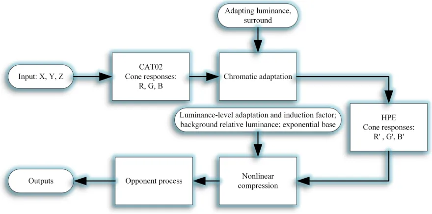
Figure 2.14Schematic diagram of the CIECAM02 computation process.

The output of CIECAM02 includes all absolute and relative color attributes. It can predict almost all

color appearance phenomena except Helson-Judd effect and Helmholtz-Kohlrausch effect [11].

2.4 Digital Still Camera Based Colorimetry

Digital still cameras are widely used nowadays in many applications, from the archiving of art works, to

medical imaging, and to quality control in manufacturing. Our research aims to utilize a digital camera

for color quality control of camouflage samples. In this section, a prototypical camera architecture

and imaging process pipeline is introduced first. The noise properties associated with this techniques

are summarized, and finally various color calibration methods, as key components of the process, are

(45)

2.4.1 Digital Camera Architecture and Pipeline

An image can be described as the variation of light intensity as a function of position on a plane, and

a digital still camera is an instrument that converts image information into digital signal and stores it.

The general configuration of a modern digital still camera is shown in Fig. 2.15 [111]. A typical process

pipeline in a consumer camera is listed below [112]:

• Exposure adjustment & optics/focus;

• Initial image capture & digitization;

• Dark noise removal & noise reduction;

• Uniformity adjustments;

• Demosaicking;

• White balance;

• Color correction;

• Tonescale (gamma correction);

• Appearance adjustments; and

• Compression/file formatting.

In a professional cameras the workflow is different from that in cameras with common usage. In the

former case the image is usually stored as lossless compressed raw data first and most of the processes

are done in the application period as needed [111].

2.4.2 Digital Camera Noise

Noise can be defined as unwanted signal fluctuations that deteriorate an image or signal. It can be

(46)

Figure 2.15Block diagram of the hardware components used in a typical digital camera [111].

2.4.2.1 Digital Camera Noise Classification

Many types of noises have been identified. They can be divided into several categories based on their

origins: illumination-independent, illumination-dependent, and digital processing noise [113, 114, 115,

116, 117, 118, 119]. Each type of noise has its own manifestation and dependency as shown in Table 2.2

[118].

• Illumination-independent noise

This type of noise includes: reset noise (NR), thermal noise (Nthermal), dark noise (Ndark),

fixed-pattern noise (NFPN) and others (Nother). The combination ofNR,NthermalandNotheris also referred

(47)

Table 2.2Classification of Digital Camera Noise [118].

Noise Type Manifestation Dependencies

Reset noise Additive temporal and spatial variance Temperature Thermal noise Additive temporal and spatial variance Temperature

Dark noise Additive temporal and spatial variance Temperature and exposure time Fixed pattern noise Additive spatial variances Temperature and exposure time Others Additive temporal and spatial variance Temperature and readout rate Photon short noise Multiplicative spatial variance Illumination

Photon response

nonuni-formity noise Additive temporal and spatial variance Illumination

Demosaicking noise Multiplicative Demosaicing implementation

and combined sensor noise

Post image-capture noise Multiplicative Parameters for image enhance-ment and combined sensor noise

Quantization noise Additive noise Image content

agitation of electrons within a resistor, it is also named by its discoverer in 1928, as Johnson noise

[120];Ndarkis due to the random generation of electrons and holes within the depletion region of

the photo-sensor; difference in detector size, doping density, and foreign matter which can cause

NFPN and which does not change over time.

• Illumination-dependent noise

Two types of noises belong to this classification: photon shot noise (NPSN), and photon response

nonuniformity noise (NPRSN).NPSN is caused by the particle nature of light, andNPRSN is due to

the nonuniformity of filter transmissivity and sensor response.NPSN is the dominant noise amongst

various noises [121].

• Digital processing noise

Bayer color filter array (CFA) is commonly used in digital cameras, thus a demosaicking process

(48)

interpolation which can cause some errors known as demosaicing noise (ND). In the process of

analog-to-digital conversion, quantization noise is introduced (NQ). Other post imaging processes,

such as image sharpening, can also result in noises denoted as (NP).

2.4.2.2 Digital Camera Noise Modeling

A large number of digital noise models have been proposed emphasizing different types of noise. Amongst

these models, the most comprehensive one was developed by Irie in 2008 [117], as shown in Eq. 2.3.

Icap= (I+NPSN+NPRSN+NFPN+Ndark+Nread)NDNP+NQ (2.3)

where Icap is the captured noisy image signal,I is sensor irradiance, other symbols are the same as

mentioned above. All noises are considered to follow a Gaussian distribution and be additive exceptNPSN

which is Poisson noise.

2.4.3 Digital Camera Color Calibration

With the improvement in image resolution, dynamic range and stability, the commercial digital cameras

can be used as colorimeters when they are properly calibrated. This will offer many advantages compared

with spectrophotometers and spectroradiometers: first the digital cameras can measure larger areas, while

radiometric systems typically deal with spot measurements; second, set up and operation of a camera is

much simpler and their cost is much lower [125, 126]. However, the inborn limitations associated with

digital cameras include the fact that their spectral responses are not linearly related to CIE CMFs. This

linear relationship is also called Luther-Ives condition [127, 128]. In addition, the camera responses are

device dependent, thus some intermediate spaces are needed for color communication.

To overcome these limitations, a color management technique (CMT) is needed. CMT can be defined

as [129]:

(49)

content data, and application of color data conversions as required to produce the intended

reproductions.

International Color Consortium (ICC)provides a color management framework which is currently the

standard as far as the reproduction of still images are concerned. The ICC was established in 1993 by

eight imaging companies [129]. Its overall workflow is shown in Fig. 2.16 [49]. The fundamental concept

of ICC workflow is to create transformations between digital devices and profile connection space (PCS,

CIEXYZ or CIELAB) which is device independent. The parameters associated with these transformations

as well as other color reproduction data such as rendering intent are stored in a file named as ICC profile.

Different ICC profiles are communicated via a ’translator’ named asColor Management Module (CMM)

which accepts parameters predefined in the ICC profile and creates transforms that subsequently convert

color coordinates from one device to another [129, 49]. The rendering intent refers to the objective of

color reproduction. The key component in the ICC profile is the transformation between systems. This is

also called color correction.

Many approaches have been proposed for digital camera color correction. These methods can be

broadly divided into two groups: target-based and model-based which are briefly discussed in the

following section [130].

2.4.3.1 Target-based Method

Target-based method refers to a practice whereby a mathematical transformation is created from camera

responses to CIEXYZ or CIELAB based on a set of training data in which the CIEXYZ and CIELAB

values are known. This process can be simply denoted asF:c07→t, whereF is the conversion function, c0= [R,G,B]T andt= [X,Y,Z]T and they represent camera responses and CIE tristimulus, respectively, which can be obtained from Eq. 2.4.

c0=STLr t=ATLr

(50)

Figure 2.16Overview of the ICC color management architecture.

whereSandAare camera’s spectral response functions and CIE CMFs, respectively.Lis a diagonal matrix and the diagonal elements are the SPD of the illuminant, andris the reflectance of the object. The SPD of the light source is usually sampled from 400 nm to 700 nm with 10 nm interval, thus

the dimension ofSandAis 31×3, and that of randLis 31×1 and 31×31, respectively. In the target-based method,cis obtained from the captured image, and the noise is ignored here.tis measured using a spectrophotometer.

The transformation functionF can be obtained from an optimization process, as shown in Eq. 2.5.

F=arg min

F ψ t,ˆt

(2.5)

whereψ(·)is the cost function which can be the mean color difference metric or the mean square error

(51)

and their variations.

• Polynomial Regression

The general mathematical formulas for polynomial regression are shown in Eq. 2.6.

X=c₁m₁₁+c₂m₁₂+· · ·+cjm1j+· · ·+ckm1k

Y=c1m21+c2m22+· · ·+cjm2j+· · ·+ckm2k

Z=c1m31+c2m32+· · ·+cjm3j+· · ·+ckm3k

(2.6)

These can be rewritten in a compact matrix form, as shown in Eq. 2.7.

ˆt=Mc (2.7)

The number of termskand the coefficientscin above functions can be varied dependent on the actual camera used and some typical forms are shown in Table 2.3.Mcan be approximated using the least square technique [111, 131], and Eq. 2.5 can be rewritten as that shown in Eq. 2.8.

M=arg min M ( 1 N N

∑

i=1

kti−Mcik2

)

(2.8)

whereNis the number of samples used to train the polynomial regression function. The solution

of Eq. 2.8 is shown in Eq. 2.9.

M=DCT(CCT)−1 (2.9)

whereD={t₁,t2, . . . ,tN}andC={c1,c2, . . . ,cN}.

Vrhelet al.[132] computed the 3×3 matrix by preserving the white point. Finlaysonet al.[133] in 1997 developed a conceptually similar method,white-point preserving least-squares fits(WPPLS).

(52)

Table 2.3The polynomial regression coefficients

Number of

terms(m) Coefficients(c)

3 R G B

4 1 R G B

6 R G B RG RB GB

8 1 R G B RG RB GB RGB

9 R G B RG RB GB R2B2G2

11 1 R G B RG RB GB R2B2G2RGB

14 1 R G B RG RB GB R2B2G2RGB R3G3B3

20 1 R G B RG RB GB R2B2G2RGB R3G3B3RG2R2G G2B B2G R2B B2R

predictions for heavily weighted colors These methods are calledweighted least-squares regression

[134, 135, 111]. Hardeberg [136] found that using the cube root of R, G and B as the input of

polynomial regression function would improve the conversion accuracy in CIELAB color space,

in a manner similar to the technique used for the CRT monitor calibration [137, 138]. Honget

al.[126] and Pointeret al.[139] systematically investigated the effect of the number of training

samples and terms in polynomial functions on the accuracy of color correction. Finlaysonet al.

[140] noted that polynomial fit depends on camera exposure time and the camera responses are

not linear, thus they proposed theroot-polynomial methodtechnique. Generally speaking, if the

spectral sensitivity of the camera filters are closer to the CIE CMFs and camera responses are

more linear then a linear transform process will give better predictions. Several metrics have been

proposed to determine the performance of digital cameras [141, 104, 142, 143, 144, 102, 145].

• Multi-dimensional Look-up Table (MLUT)

MLUT method is a technique whereby one space is converted to another employing both

inter-polation and extrainter-polation techniques from the geometrical aspects of the color space. Trussell

(53)

used for a digital camera can be mathematically denoted asL[ci,f(ci),I(c)], where{ci}are

samples in the camera RGB space,{f(ci)}are the corresponding function values in the CIE XYZ

or CIELAB color space, and I(c)is the function or algorithm used to calculate the value in a device independent color space using the interpolation or extrapolation method. The general

procedure for the MLUT method is as follow:

1. Creation of a look-up table from a color chart

Suppose the aim is to create a 3 dimensional look-up table withNuniformly sampled points

at each axis of the RGB color space which is usually considered to be a cube. It is impractical

to generate real samples at each grid, thus a color chart sampled in a color space is needed.

Thecvalue at each grid in the RGB color space and corresponding f(c)value in the CIE XYZ or CIELAB color space can be computed using a linear interpolation or polynomial

regression method or other methods based on its neighboring samples from the color chart

and grids of which the f(c)values are known from the previous computation step. Finally, a 3-D LUT is obtained and thecvalue of a point can be converted to its coordinates in the LUT.

2. Extraction and Interpolation

Once a new point with knownc value is obtained, its neighboring grids can be extracted easily, and finally geometric interpolation techniques including bilinear, trilinear, prism [146],

pyramid and tetrahedral interpolation [147] or the same interpolation methods used to create

MLUT can be used to compute its f(c)value. One example is provided to illustrate how to do interpolation using a trilinear interpolation method [131]. The point of interest is pas

shown in Fig. 2.17. The nearest eight grid points in MLUT are denoted as p000to p111as

illustrated in Fig. 2.17. Letp₀₀₀denotes the coordinate of pointp₀₀₀(x₀,y₀,z₀)in MLUT, and

[x₀,y₀,z₀]are the corresponding coordinates in the device independent color space.

(54)

from their two nearest grids, then the f(c)value of pointsp1andp2are obtained from their neighboring points in the previous step using linear interpolation. Finally, linear interpolation

is used again to compute f(c)value of point p. The computation can be denoted in matrix form as shown Eq. 2.10.

f(c) =QTBP (2.10)

where vector Q= [1 ∆x ∆y ∆z ∆x∆x ∆y∆z ∆z∆x ∆x∆y∆z]T, and Matrix B is shown in Eq. 2.11. MatrixP= [p000 p001 p010 p011 p100 p101 p110 p111]T.p000 is a 3×1 vector.∆x=x1−x0,∆y=y1−y0and∆z=z1−z0.