Development of Soft Subgrade Undercut Criteria and Response with Stabilization Measures.

(1)

ABSTRACT

PARK, YOUNG JIN. Development of Soft Subgrade Undercut Criteria and Response with Stabilization Measures. (Under the direction of Dr. Mohammed A. Gabr, and Dr. Roy H. Borden.)

The stability of subgrade soils is a concern during roadway construction, and as such, inappropriate soft subgrade soils often must be replaced by stabilized materials in an undercut. Systematic and quantifiable undercut criteria are established based on the strength

and stiffness parameters of the subgrade soil, and these parameters are based on the loads caused by proof roll trailers and other construction vehicles. Once such criteria are

established, and the state of the subgrade soil is determined, engineers can determine the particular situations that require undercutting and stabilization. That is, these criteria provide engineers with the required degree of stability and the magnitude of settlement, as

determined by the stiffness and strength parameters obtained from field and laboratory testing. The criteria proposed are a bearing capacity ratio of 2.0 inches and a 1.0-inch

settlement for pumping and rutting. By investigating the mechanistic behavior of elastic-perfectly plastic media, the pumping and rutting criteria for soft or stabilized subgrade soils can be identified and discussed based on proof rolling test results. Rutting is associated

(2)

employed uses backcalculated stiffness factors to yield displacements that agree with those

measured during the tests, although the elastic-perfectly plastic model does not present a consistent prediction under external stress. The stabilization methods are investigated for field sections where undercutting is typically performed. As the widening embankment fill is

(3)

Development of Soft Subgrade Undercut Criteria and Response with Stabilization Measures

by Young Jin Park

A dissertation submitted to the Graduate Faculty of North Carolina State University

in partial fulfillment of the requirements for the degree of

Doctor of Philosophy

Civil Engineering

Raleigh, North Carolina

2010

APPROVED BY:

(4)

DEDICATION

(5)

ACKNOWLEDGEMENTS

I would like to express my deep gratitude to my advisor and committee chair, Dr. Mohammed A. Gabr, for his direction and support during the course of this study. I know I could not have come this far without his support and encouragement. Also, I greatly

appreciate the teaching and sincere words of encouragement from my committee co-chair, Dr. Roy H. Borden. I will always remember the moment I met him in the first CE548 class.

Many thanks are also extended to Dr. M. Shamimur Rahman and Dr. T. Matthew Evans for their role on my review committee and their interest in my work.

During the years it took me to write this dissertation, I have been helped and

encouraged by many people in ways both small and large. However, several people must be singled out for special thanks: Brent Robinson, Ben Possiel, Wansoo Kim, Jong Koo Jeon,

Sharmir Nadia, Heoseon Yeom, Xueling Zhao, Sangchul Pyo, Ben Cote, Jaehun Ahn, Mohammad Can Ulker, Zhangwei Ning, Matt Ranando, Edwin Jones, Mahdi Bahador, Jeremy Kress, Hamed Mojarrad, and Cheng Wang.

To my family: Mom, Dad, Eun A, Young Hun, and Kyeong A, I do not have enough words to express my deep gratitude for your support and prayers. Each of you has sacrificed for me over the course of the years. A man is nothing without his family; I am living proof of

(6)

BIOGRAPHY

Young Jin Park was born January, 7, 1970 in Seoul, Korea, to Jung Nam Park and Jeom Sook Jung. He received his B.S. and M.S. degrees in Civil Engineering from Korea University in 1997 and 1999, respectively. After earning his M.S. degree, Young Jin worked

with the Daebon Engineering Company as an engineer from July 1999 to November 2000, and with Sambo Engineering Company as a project engineer from December 2000 to March

(7)

LIST OF FIGURES

Figure 1. Flow chart of the study and the relationships of the various

study components ··· 5 Figure 2. Typical field conditions under which undercutting typically

occurs ··· 9 Figure 3. Comparison of effective friction angles predicted by PI values

and obtained from triaxial tests ··· 38 Figure 4. Range of elastic modulus values found in the literature (Huang,

2004; Brunton et al., 1992; CROW, 1998; Evdorides & Snaith,

1996): (a) subgrade soil layer, and (b) ABC layer ··· 42 Figure 5. Determination of initial elastic modulus values from hyperbolic

curves: (a) initial tangential modulus and secant modulus, and (b)

relation to confining stress ··· 44 Figure 6. Inverse analysis scheme ··· 51 Figure 7. Forward models of the test pits used for inverse analysis ··· 57 Figure 8. Pressure and vertical displacement plots for static load tests of

the test pit ··· 61 Figure 9. Extraction of elastic portions from the pressure and

displacement curves (test 9): (a) linear regression of each loading

step, and (b) final input after calibration ··· 62 Figure 10. Loading and unloading curves obtained from the static load

test results: (a) test 9 and test 20, and (b) test 15, test 16, and test

17 ··· 64 Figure 11. Pressure vs. vertical displacement for the measurements: (a)

(14)

Figure 14. Excessive plastic displacement occurred in the inverse analysis: (a) load and displacement, and (b) displacement as

friction angle increases ··· 70 Figure 15. Elastic modulus values and strength parameters backcalculated

based on displacements in the homogeneous plastic model: (a) comparison of elastic and plastic models, and (b) strength

parameters obtained from inverse analysis ··· 71 Figure 16. Displacement in the forward models with parameters

backcalculated based on displacements in the homogeneous plastic model for test cases ··· 73 Figure 17. (a) Pressure vs. displacement plots for comparing forward

models with parameters backcalculated in the layered elastic

models, and (b) ratio of elastic modulus values for each layer ··· 75 Figure 18. Correlation of elastic modulus values for stabilized layers with

a homogeneous model: (a) elastic modulus values with ABC, and

(b) elastic modulus values with stabilized layer ··· 78 Figure 19. Displacements of forward model with backcalculated

parameters ··· 81 Figure 20. Backcalculated elastic modulus values and strength parameters

in the ABC: (a) elastic modulus, and (b) strength parameters ··· 83 Figure 21. Pressure profiles of forward model with the parameters

backcalculated based on pressure and displacement in the layered

model ··· 86 Figure 22. Displacements of forward model with the parameters

backcalculated based on pressure and displacement in the layered

model ··· 88 Figure 23. Errors for each test according to the plastic models in inverse

analysis ··· 91 Figure 24. (a) Displacements on undercut criteria chart, and (b) bearing

capacity for c/pa = 0.1 in. and c/pa = 0.3 in. ··· 92 Figure 25. Load vs. displacement curves for proof rolling data ··· 95 Figure 26. Application of undercut criteria to the properties obtained from

(15)

Figure 28. Axisymmetric model: (a) three-dimensional axisymmetric

condition, and (b) stress condition ··· 113 Figure 29. Stress-strain relationship of elastic-perfectly plastic model ··· 114 Figure 30. Loading function and displacement response: (a) haversine

load function of proof roller, and (b) typical displacement plot on

time ··· 118 Figure 31. Proof roller trailer: (a) typical proof roller used by the

NCDOT, and (b) dimensions of wheel and tires applied on

subgrade soil ··· 120 Figure 32. (a) Deformed wheel configuration, and (b) distribution of

flexibility factor, for the different strengths ··· 121 Figure 33. (a)Deformed model and contours of vertical displacement, and

(b) estimation of bearing capacity in deformation-controlled

method ··· 122 Figure 34. (a) Deformed model and contours of vertical displacement,

and (b) estimation of bearing capacity in pressure-controlled

method ··· 123 Figure 35. Pressure and displacement plots dependent on strength and

stiffness: (a) E/pa = 25, and (b) c/pa = 0.7 ··· 126

Figure 36. Bearing capacity plots for E/pa = 50 ··· 130 Figure 37. Capacity ratios according to elastic modulus values: (a) = 0,

and (b) = 20 degrees ··· 132 Figure 38. Normalized cohesion vs. factor of safety for axisymmetric

condition ··· 134 Figure 39. Design criteria charts based on the maximum shear strain at

the boundary of the loading plate: (a) = 0 degree, and (b) = 20

(16)

Figure 44. Estimation of the model prediction for the deformation curves in the axisymmetric condition: (a) using Eq. (19), and (b) using

Table 43 ··· 143 Figure 45. Design criteria charts for the axisymmetric condition ··· 144 Figure 46. Design charts for proof roller loading: (a) pumping (maximum

settlement), and (b) rutting (permanent settlement) ··· 145 Figure 47. Design charts for rutting (permanent settlement) in the proof

rolling loading ··· 147 Figure 48. Bearing capacity plots for the case of E/pa = 50 ··· 149

Figure 49. Capacity factors according to elastic modulus values: (a) = 0,

and (b) = 20 degrees ··· 150 Figure 50. Normalized cohesion vs. factor of safety for plane strain

condition ··· 152 Figure 51. (a) Coefficient, a0, and (b) a1 for the plane strain condition ··· 154

Figure 52. The coefficient, a2, of the model ··· 154 Figure 53. (a) Coefficient, a1 and (b) a2, of the model for the plane strain

condition ··· 156 Figure 54. Estimation of the model prediction for the deformation curves

under the axisymmetric condition: (a) using Eq. (22), and (b) using Table 46 ··· 157 Figure 55. Design criteria charts for plane strain condition ··· 159 Figure 56. Undercut charts for proof roller loading for the plane strain

condition: (a) pumping (maximum settlement), and (b) rutting

(permanent settlement) ··· 160 Figure 57. Comparison of maximum and permanent displacements for the

axisymmetric and plane strain condition ··· 161 Figure 58. Design charts for rutting (permanent settlement) in the proof

roller loading ··· 162 Figure 59. Resilient displacement for plane strain condition: (a)

time-dependent displacement plot, and (b) normalized displacement

plot on cohesion axis ··· 163 Figure 60. Normalized pumping deformation curves under proof roller

(17)

Figure 61. Pumping deformation plots for plane strain condition: (a) for

friction angles, and (b) trend line and elastic solution plot ··· 166

Figure 62. Application of undercut criteria for the subgrade soil and stabilization ··· 169

Figure 63. Empirical correlation of DCPI vs. undrained shear strength and resilient modulus values: (a) undrained shear strength (Gabr et al., 2010), and (b) resilient modulus (Mohammad et al., 2007) ··· 170

Figure 64. Samples located in undercut design chart: (a) axisymmetric condition, and (b) plane strain condition ··· 171

Figure 65. (a) Static Load Sequences, and (b) One Cycle of Proof Roller Loading ··· 186

Figure 66. Numerical models of the test pits used for the simulations ··· 188

Figure 67. Three different models ··· 192

Figure 68. Simulated models with various thicknesses ··· 193

Figure 69. Comparison of three modeling methods: (a) ratio of bearing capacity, and (b) ratio of displacement ··· 194

Figure 70. Vertical displacement profiles of the model with 9-inch ABC: thickness for each reinforcement method ··· 195

Figure 71. Ratio of mobilized pressures assuming axisymmetric versus plane strain conditions at a uniform displacement ··· 197

Figure 72. Applying pressure and displacement plots for large-scale tests ···· 201

Figure 73. Displacement results of the cases of proof roller testing ··· 203

Figure 74. Project section and corresponding idealization for numerical model: cases 1 and 2 ··· 206

Figure 75. Dimensions, construction sequences, and numerical mesh: case 1 ··· 207

(18)

Figure 81. Bearing capacity analysis: (a) comparison with Prandtl’s

solution, and (b) displacement plot with magnified mesh ··· 215 Figure 82. Displacement and mobilized pressure curves ··· 217 Figure 83. Bearing capacity for the cases ··· 218 Figure 84. Ratios of the bearing capacity of the stabilization methods to

the non-stabilization method ··· 219 Figure 85. Settlements of each stabilization method for all field

conditions ··· 220 Figure 86. Effectiveness of the stabilization methods ··· 221 Figure 87. Settlement at the center of proof roller according to time

sequence ··· 222 Figure 88. Permanent settlements for proof roller loading ··· 223 Figure 89. Maximum displacement for proof roller loading ··· 224 Figure 90. Vertical displacement contours and vectors of case 1 model:

(a) stabilized by geotextile (HP570), and (b) stabilization by lime

amendment ··· 225 Figure 91. Strain distribution of geotextile (HP570) for each stabilization

method ··· 226 Figure 92. Y-Direction displacement profiles for each stabilized method

of case 1: (a) before adding fill, and (b) after adding fill ··· 227 Figure 93. Stress increase with depth for various stabilization measures

(case 1): loading imposed by the fourth lift and 60 psi surface

(19)

LIST OF TABLES

Table 1. Index Properties for Subgrade Soil and Stabilization Measures ··· 34

Table 2. Typical Effective Angle of Internal Friction for Unbound Granular and Subgrade Materials ··· 36

Table 3. Results of Triaxial Tests for Piedmont Residual Soil (NCDOT) ··· 37

Table 4. Basic Statistics of Results of Triaxial Tests for Subgrade Soil ··· 37

Table 5. Results of Triaxial Tests for Coastal Plain Soil ··· 39

Table 6. Elastic Modulus Values and Poisson’s Ratios, as Found in the Literature ··· 40

Table 7. Elastic Modulus Values for Various Soil Types, as Found in the Literature ··· 41

Table 8. Poisson Ratios for Various Soil Types, as Found in the Literature ··· 43

Table 9. Stiffness and Strength Parameters Used in the Analysis ··· 46

Table 10. Combination of Categories of Inverse Analysis ··· 60

Table 11. Subgrade Response Modulus (K) and Displacement at Each Loading Step Obtained from the Tests ··· 63

Table 12. Total Displacement of Each Loading Stage for the Elastic-Perfectly Plastic Model ··· 63

Table 13. Input Subgrade Response Modulus Value (K) and Elastic Modulus Value (E) Determined from Backcalculation for Homogeneous Elastic Media for Each Test ··· 68

(20)

Table 18. Equivalent Elastic Modulus Values for Stabilized Layers and

the Ratio of the Modulus to the Subgrade Layer ··· 77

Table 19. Strength Parameters Backcalculated for Layered Plastic Models ··· 79

Table 20. Settlements Observed in the Test Pit and Predicted in the Elastic-Perfectly Plastic Model ··· 80

Table 21. Stiffness and Strength Parameters Backcalculated in Each Loading Step for Test Cases ··· 82

Table 22. Measured and Predicted Pressure Levels in Three Load Cells for Test 9 ··· 84

Table 23. Measured and Backcalculated Pressure Levels in Three Load Cells for Test 15 ··· 85

Table 27. Measured and Backcalculated Displacements on the Surface for Test Cases ··· 87

Table 28. Summary of Material Properties Evaluated by Inverse Analysis ···· 89

Table 29. Errors in the Inverse Analysis ··· 90

Table 30. Normalized Elastic Modulus and Cohesion Values Determined from a Single-Layer System ··· 91

Table 31. Displacements of Proof Roller Loading at Loading Time of 1.0 second ··· 93

Table 32. Observed and Predicted Displacements ··· 94

Table 33. Backcalculated Parameters ··· 96

Table 34. Material Properties Used in the Design Criteria Analysis ··· 115

Table 35. Number of Cases According to Strength Parameters ··· 119

Table 36. Classification of Numerical Simulations for Design Criteria ··· 127

(21)

Table 38. Estimation of Ultimate Bearing Capacity by Terzaghi and

Vesic Methods ··· 133

Table 39. Four Functions Tested for Model Development ··· 136

Table 40. Data Used in Model Fitness Tests ··· 137

Table 41. Results of Model Fitness Tests ··· 137

Table 42. Coefficients of Model for Axisymmetric Condition ··· 139

Table 43. Coefficients (a0, a1, and a2) of the Model for the Deformation Curves ··· 140

Table 44. Estimation of Ultimate Bearing Capacity by Terzaghi and Vesic Methods ··· 151

Table 45. Coefficients of Power Function Model for Plane Strain Condition ··· 153

Table 46. Coefficients (a0, a1, and a2) of the Model for the Deformation Curves under the Plane Strain Condition ··· 155

Table 47. Normalized Pumping Deformation Values for Each Friction Angle ··· 166

Table 48. Results of CU Triaxial Testing for Mixed Coastal Plain Subgrade Soil and Predicted Settlements ··· 168

Table 49. DCPI Values and Correlated Parameters: Demonstration of Undercut Criteria Using Field Data ··· 171

Table 50. Previous Research Using Numerical Programs ··· 183

Table 51. Input Parameters Used in the Analysis ··· 189

Table 52. Elastic Modulus Values Used in the Simulations for the Static Load Tests in the Test Pit ··· 190

Table 53. Material Properties for Modeling Geosynthetics and Interface Materials ··· 192

Table 54. Typical Sections of Field Cases ··· 205

(22)

LIST OF EQUATIONS

(23)

INTRODUCTION

(24)

The main objectives of this study are to develop a systematic approach for determining whether or not undercutting is necessary, and to investigate the adequacy of stabilization measures typically employed if undercutting is deemed necessary. This study is undertaken to accomplish the following objectives:

i) Systematic undercut criteria, which specify the situations in which subgrade soil should be undercut, will be established based on mechanistic modeling and under conditions for typical traffic and proof rolling loads. Dynamic modeling will be applied to simulate proof rolling on the subgrade, and an ultimate bearing capacity will be implemented to indicate the factor of safety under the applied loads. Pumping behavior and the rut depth of the subgrade soil will be evaluated based on the developed criteria. Models will be developed and implemented to obtain the curves for these criteria, and the mechanistic significance of these curves will be determined. ii) Test pits for investigating the behavior of the undercut and stabilized subgrade soil

will be simulated numerically, and the material properties of the soils will be determined by the resultant measurements and inverse analysis. The loads applied at the test pits will consist of static, proof roller, and cyclic loads. Of these loads, the proof roller and cyclic loads are simulated in the dynamic model.

(25)

BACKGROUND

The North Carolina Department of Transportation (NCDOT) initiated a research project, “Establishment of Subgrade Undercut Criteria and Performance of Alternative Stabilization Measures” (Gabr et al., 2010), to establish the criteria required for making appropriate decisions with regard to undercutting and suitable stabilization methods and to reduce the amount of undercutting by applying the most suitable select material, ABC, geosynthetic reinforcement, and/or lime stabilization method. The tasks undertaken by the researchers were designed to: i) review current NCDOT practice, ii) establish factors that define the need for undercutting using in situ testing techniques, iii) implement numerical modeling of short-term and long-term conditions, and iv) develop guidelines for alternative and/or supplemental approaches to undercutting, including the use of geosynthetics and chemical stabilization. Undercut criteria based on a mechanistic approach were developed in this research, and dynamic and static numerical models were implemented for simulating test pits and typical field sections. The task of establishing these undercut criteria and numerical models is the primary (or main) focus of this study

PROBLEM STATEMENT

(26)

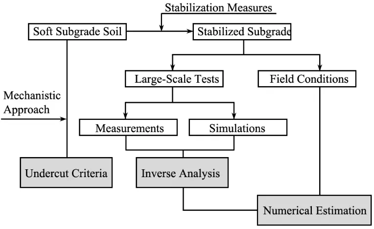
impact of the resultant stabilization measures. In brief, the first part is the determination of the mechanistic properties of the material used in the simulated test pit. The second part is the development of the mechanistic-based undercut criteria. The third part is the application of the material in field conditions based on NCDOT practice.

(27)

Figure 1. Flow chart of the study and the relationships of the various study components

Assessment of Stiffness and Strength Parameters of Soft Subgrade Soils with

Stabilization Using Inverse Analysis

Twenty-two plate load tests under static, proof roller, and cyclic traffic loads were performed in a test pit, and each test section consisted of soft subgrade soil and stabilized layers. Load cells were embedded, and the stresses mobilized by the external loads were measured. The settlement under the loads and the deformation of the subgrade soil also were monitored (Gabr et al., 2010).

(28)

used in numerical modeling, are dependent upon the degree of compaction for both the subgrade and stabilized layers and the water content of the subgrade soil layer. Other issues, such as the appropriateness of the use of constitutive models to simulate the plastic behavior of the soil, interactions of the multilayered soil layers, and hardening or softening effects beyond the onset of the yield point can cause errors in the prediction.

Nevertheless, it is known that the predictions are in approximate agreement with the measurements under a specific condition in which the numerical issues do not occur. Static load tests can be regarded as providing this specific condition, and results of such tests suggest that the behavior of soil in the test pit is dependent mainly on the variation of the material properties. From the measured stress and displacement values obtained from the static load tests, the material properties can be backcalculated. By applying inverse analysis to the results of the static load test conducted in the test pit, the stiffness and strength parameters can be assessed, and the magnitude of the strength for the stabilized soil layer can be evaluated.

Three factors were considered in the inverse analysis:

i) Assuming the layered large-scale test section to be a homogeneous soil layer can lead to finding the equivalent properties and enable the estimation of the magnitude of stabilization on the undercut criteria chart.

ii) According to a combination of data, different material properties can be determined, and thus, optimized values can be selected for the numerical simulations.

(29)

As an appropriate numerical scheme, the finite difference method is used to simulate the test pit, and the Levenberg-Marquardt optimization algorithm is adopted in the backcalculation process used to obtain the parameters.

Soft Subgrade Undercut Criteria, Including Rutting and Pumping Responses

The engineering approach taken to ascertain the stability of the subgrade soil is based on the estimation of the soil’s strength and stiffness (Thompson, 1979). That is, from a site investigation, the strength and stiffness values can be estimated, and engineers can then determine whether or not undercutting is needed and the type of stabilization method that is required for the subgrade soil. The undercut criteria will address the following issues:

i) Quantifiable criteria must be developed to determine the state of the subgrade soil and to aid in making the decision whether or not to undercut and, if undercutting is deemed necessary, which stabilization method is most appropriate for the circumstance.

ii) The criteria must be applicable for the external loads that are caused by construction vehicles and proof roll trailers.

(30)

Field Applications of the Undercut Criteria and the Impact of the Stabilization

Measures

One of the main objectives of conducting the twenty-two tests in the test pit is to evaluate each stabilization method in terms of relative effectiveness and appropriateness. The numerical computations for these tests were designed to provide mechanistic information about the test sections, which can then be extended to the prediction for other factors, such as different depths of the undercut and/or a complex geometry in the field. This objective consists of two tasks. One is the simulation of tests performed in the test pit, and the other is the application of the stabilization method in field cases. Results from the simulations of large-scale tests can be extrapolated to the field cases.

Out of the twenty-two large-scale tests, five representative stabilization methods were selected whereby the stabilization is accomplished using a select fill material, an ABC material, geotextile (HP570) with ABC, geogrid (BX1500) with ABC, or lime-stabilized soil. Static, proof roller, and cyclic traffic loads were applied on the surface of the test pit using a steel plate with a flexible rubber pad to make the loads uniform. Settlement and stress levels were measured at load cells embedded in the subgrade soil layer.

(31)

and plastic deformation that can compromise their function. An example of such soils can be found within the Triassic basins of North Carolina.

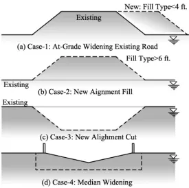
Four field conditions, under which undercutting generally is necessary, were simulated numerically. Schematic drawings of these typical undercut sections, as issued by NCDOT engineers, are shown in Figure 2 and represent (a) a fill section, (b) deep subgrade soils in a cut section, (c) the widening of an existing embankment, and (d) the widening of a median section.

(32)

this type of section include the presence of shallow groundwater and soft subgrade near the embankment as well as the confining effect caused by the existing embankment.

Case 2, shown in Figure 2 (b), represents the construction of a new alignment in a fill situation. The numerical model mesh and construction sequences are almost the same as in Case 1, with one difference, which is the absence of an existing embankment. Similarly, a high groundwater table condition and soft subgrade suggest that the decision to undercut should be made. Further, heavy and repetitive hauling can also cause deterioration of the fill section's subgrade stability. Typical sections for Case 1 and Case 2 are found in the R-2510A NBL project.

Case 3, shown in Figure 2 (c), represents a new alignment in a cut situation. A typical section for numerical simulation is taken from project U-2524AB, and the depth of the undercut is determined by the level of moisture and the depth of the groundwater table. Because the soft subgrade soil in this cut section is saturated, lime stabilization is typically the type of stabilization method that is implemented.

(33)

ORGANIZATION

The section entitled ‘Assessment of Stiffness and Strength Parameters of Soft Subgrade with Stabilization Measures Using Inverse Analysis’ explores the characteristics of the material used in the large-scale tests. The material properties used for the numerical simulations in this study will be determined by consulting the literature and laboratory test results. Triaxial testing will be used to assess the hardening effects for the strength parameters. This section also presents the inverse analysis of the test pits that have been stabilized using the five undercut methods. The Levenberg-Marquardt algorithm will be adapted in this study to minimize the error between the predictions obtained from the model and the actual measurements.

The section entitled ‘Soft Subgrade Undercut Criteria, Including Rutting and Pumping Responses’ presents the undercut criteria for design traffic and proof roller loads, which are simulated under axisymmetric and plane strain conditions, respectively. Undercut criteria consist of bearing capacity curves and deformation curves; the empirical models for the deformation curves are developed and their significance discussed in this section. Furthermore, this section presents the characterization of pumping and rutting, which is implemented based on the criteria, and also presents the applications of the undercut criteria.

(34)

(35)

REFERENCES

Gabr, M. A, Borden, R. H. (2006). “Proposal of Development of Undercut Criteria and Alternatives for Subgrade Stabilization.” North Carolina Department of Transportation.

Gabr, M. A., Borden, R. H., Robinson, B. R., Cote, B. M., Park, Y. J., Pyo, S. (2010). “Establishment of Subgrade Undercut Criteria and Performance of Alternative Stabilization Measures.” Department of Civil, Construction, and Environmental Engineering, North Carolina State University, in cooperation with the North Carolina Department of Transportation. North Carolina State University, Raleigh, NC (March).

Holtz, R. D., Christopher, B. R., and Berg, R. R. (1998). “Geosynthetic Design and Construction Guidelines.” FHWA Publication No. HI-95-038. Federal Highway Administration, Washington, D.C., 459 pages.

Thompson, M. (1979). “Subgrade Stability.” Transportation Research Record 705, Subdrainage and Soil Moisture, pp. 32-41.

(36)

(37)

LITERATURE REVIEW

A survey of the literature has been undertaken to review the state of practice and recent findings for the subject of this study. This section summarizes the stability of subgrade soil, which is related to undercutting and stabilization, the characteristics of the subgrade soil used in the large-scale testing in terms of engineering properties, the inverse problem that exists between the measurements and the predictions, and the application of numerical simulations, as found in previous research.

Soft Subgrade Undercut Criteria, Including Rutting and Pumping Responses

(38)

performance of the completed pavement. These procedures are now commonly referred to as undercutting and stabilization.

For the design or construction process, an empirical design manual for unpaved roads has been adopted by engineers to ascertain the depth of the undercut and the appropriate stabilization method. Croney (1977) considered the upper 60 cm (2 feet) of the subsurface soil matrix as the subgrade layer, and regarded this dimension as a meaningful depth with respect to strength. Hammit (1970) developed an empirical formula to present the depth of a granular layer by considering the number of traffic passes, the applied load, the tire contact area, and the CBR Several empirical formulas have been suggested (Webster and Alford, 1978; Giroud and Noiray, 1981; Greenstein and Livneh, 1981; Giroud et al., 1984; Powell et al., 1984) using strength (CBR or undrained shear strength), number of traffic passes, and application of the axle load. These research efforts have led to the determination of the appropriate stabilization method for the subgrade soil as well as the depth of the undercut.

Giroud and Noiray (1981) presented the most well-known design method for geotextile-reinforced unpaved roads, which calculates the depth of the granular layer under an approximated geometry of stress distribution. Giroud and Han (2004 and 2004b) proposed a new empirical design model for geogrid-reinforced unpaved roads, which is calibrated by the experimental data and considers the interaction between the geogrid and an ABC, and the number of traffic loading cycles.

(39)

the subgrade and sub-base layers. Several national guidelines and manuals are available for the use of geosynthetics for paved roads. The FHWA (Federal Highway Administration) specifications by Holtz et al. (1998), the Geosynthetic Materials Association (GMA) White Paper II by Berg et al. (2000), and AASHTO PP 46-01 (AASHTO, 2001) also provide guidelines for base course reinforcement using geosynthetics.

Berg et al. (2000) considered three design factors – Base Course Reduction (BCR), Traffic Benefit Ratio (TBR), and Layer Coefficient Ratio (LCR) – for the geosynthetic reinforcement of a base course. The BCR indicates the percentage of reduction in the thickness of the base layer that is caused by the reinforcement, the TBR is used to define the magnitude of improvement of the reinforcement in terms of the number of load cycles, and the LCR is used to compare the reinforced versus unreinforced cross-section performance by modifying the base course portion of the AASHTO structural number equation. These factors, however, do not have a mechanistic basis, and must be defined by laboratory tests that have been correlated to a field section for a particular reinforcement (Gabr et al., 2010).

(40)

Assessment of Stiffness and Strength Parameters of Soft Subgrade with Stabilization

Measures Using Inverse Analysis

Backcalculation and inverse analysis have been improved with the development of nondestructive deflection testing (NDT) and the optimization method. The observed data from various transducers reveal the response of a medium to an external factor, and the model that simulates the medium can be optimized by inverse analysis. Thompson (1992) categorized the backcalculation according to NDT measures and suggests backcalculation procedures as follows:

i) identify the relationship between the modulus of the subgrade reaction modulus (typically designated by K) and the elastic modulus,

ii) establish a database and employ iterative procedures to predict the deflection using the assigned layer modulus values,

iii) employ the spectral analysis of surface waves (SASW) technique to identify the material properties and the thickness of the layers, and

iv) initiate an expert system as a backcalculation procedure.

The iterative procedure and the techniques for minimizing the error that may arise in the process have been developed in the area of NDT and/or field scale tests.

(41)

so-called well posed in that the problem has a solution, and the solution is unique and is a continuous function of the problem data (Hadamard, 1902; Oliver et al., 2008). On the other hand, some problems that naturally occur are not well posed, and therefore are said to be ill posed. These ill-posed problems refer to inverse problems. Kubo (1992) classified the inverse problems related to field problems and their solutions.

Field Applications of the Undercut Criteria and the Impact of Stabilization Measures

Numerical analysis is a technique used to calculate the mechanical behavior of roadway components using the required material properties and constitutive models. In contrast to design methodologies that are based on empirical relationships, numerical methods have the advantage of being able to incorporate various loading configurations, environmental conditions, and complicated nonlinear models (Masad and Scarpas, 2007).

(42)

commercial programs such as ABAQUS and FLAC to simulate field conditions. The following portion of the literature review focuses on the previous numerical approaches and their simulation of roadway cross-sections.

Schwartz (2002) categorized the numerical methods for determining the stresses, strains, and deformations in flexible pavement systems. Schwartz (2002) considered three aspects to determine an appropriate pavement structural response model: 1) material nonlinearity for simulating viscoelastic materials for the asphalt concrete layer, 2) analysis dimensionality for rigorously analyzing in situ composite pavement and loading conditions, and 3) the computational practicality of performing a complicated three-dimensional finite element model.

For flexible pavement systems, it can be assumed that in situ pavements have been constructed under various mechanical and environmental conditions. So, many researchers have tried to simulate the behavior of such pavement systems using their own constitutive model. Recently, Desai (2007) suggested the disturbed state concept (DSC), which provides a modeling approach that includes various responses, such as elastic, plastic, creep, microcracking and fracture, softening, and healing under mechanical and environmental (thermal, moisture, etc.) conditions within a single unified and coupled framework.

(43)

developed using specific constitutive models. The advantages of a three-dimensional approach include the ability to consider multiple wheel loads as well as to estimate the moving and flexible behavior of actual wheel loads (Zaghloul and White, 1993; Mallela and George, 1994; Gunaratne and Sanders, 1996; Blab and Harvey, 2002). However, axisymmetric models are still reliable for analyzing the mechanical behavior of ESWLs under laboratory conditions, and as part of NDT; e.g., the falling weight deflectometer (FWD) (Al-Khoury, 2007). Using a three-dimensional finite element program (ABAQUS), Zaghloul and White (1993) simulated the dynamic behavior of multilayered pavements under traffic loading, and compared the results with those of an elastic multilayer analysis program called Bitumen Structures Analysis in Roads (BISAR).

(44)

REFERENCES

AASHTO. (2001). “Geosynthetic Reinforcement of the Aggregate Base Course for Flexible Pavement Structures.” AASHTO Provisional Standards, PP 46-01. American Association of State Highway and Transportation Officials, Washington, D.C.

Al-Khoury, R., Scarpas, A., Kasbergen, C., and Blaauwendraad, J. (2007). “Nonhomogeneous Spectral Element for Wave Motion in Multilayer Systems.” International Journal of Geomechanics, 7 (5), pp. 362-370.

Ayres, M. (1997). “Development of a Rational Probabilistic Approach for Flexible Pavement Analysis.” Ph.D. dissertation, University of Maryland, College Park, MD.

Berg, R. R., Christopher, B. R., and Perkins, S. (2000). “Geosynthetic Reinforcement of the Aggregate Base/Subbase Courses of Pavement Structures.” Geosynthetics Materials Association. Roseville, MN. http://www.gmanow.com/pdf/WPIIFINALGMA.pdf .

(45)

Boussinesq, J. (1885). “Application des Potentiels a L’etude de L’equilibre et du Mouvement des Solids Elastiques.” Gauthier-Villars, Paris.

Broms, B. B. (1965). “Effect of Degree of Saturation on Bearing Capacity of Flexible Pavements.” Highway Research Record 71, pp. 1-14.

Chen, D. H., Zaman, M., Laguros, J., and Soltani, A. (1995). “Assessment of Computer Programs for Analysis of Flexible Pavement Structures.” Transportation Research Record 1482, Transportation Research Board, National Research Council, Washington, D.C., pp. 123–133.

Croney, D. (1977). “The Design and Performance of Road Pavements.” Her Majesty’s Stationery Office, London.

(46)

Doddihal, S. R. and Pandey, B. B. (1984). “Stresses in Full-Depth Granular Pavements.” Transportation Research Record 954, Transportation Research Board, National Research Council, Washington, D.C., pp. 94-100.

Gabr, M. A., Borden, R. H., Robinson, B. R., Cote, B. M., Park, Y. J., and Pyo, S. (2010). “Establishment of Subgrade Undercut Criteria and Performance of Alternative Stabilization Measures.” Department of Civil, Construction, and Environmental Engineering, North Carolina State University, in cooperation with the North Carolina Department of Transportation. North Carolina State University, Raleigh, NC (March).

Giroud, J. P. and Noiray, L. (1981). “Geotextiles-Reinforced Unpaved Road Design.” ASCE, Journal of Geotechnical Engineering, 107 (9), pp. 1233-1253.

Giroud, J. P., Ah-Line, C., and Bonaparte, R. (1984). “Design of Unpaved Roads and Trafficked Areas with Geogrids.” Proceedings of the Conference on Polymer Grid Reinforcement. London, U.K. (March 23-24), pp. 116-127.

(47)

Giroud, J. P. and Han, J. (2004a). “Design Method for Geogrid-Reinforced Unpaved Roads – Part I: Theoretical Development.” ASCE Journal of Geotechnical and Geoenvironmental Engineering, 130 (8), pp. 776-786.

Giroud, J. P. and Han, J. (2004b). “Design Method for Geogrid-Reinforced Unpaved Roads – Part II: Calibration and Verification.” ASCE Journal of Geotechnical and Geoenvironmental Engineering, 130 (8), pp. 787-797.

Greenstein, J. and Livneh, M. (1981). “Pavement Design of Unsurfaced Roads.” Transportation Research Record 827, Transportation Research Board, National Research Council, Washington, D.C., pp. 21-26.

Gunaratne, M. and Sanders, O., III. (1996). “Response of a Layered Elastic Medium to a Moving Strip Load,” International Journal for Numerical and Analytical Methods in Geomechanics., 20 (3), pp. 191 – 208.

(48)

Holtz, R. D., Christopher, B. R., and Berg, R. R. (1998). “Geosynthetic Design and Construction Guidelines.” FHWA Publication No. HI-95-038. Federal Highway Administration, Washington, D.C., 459 pages.

Huang, Y. H. (2004). “Pavement Analysis and Design.” (2nd edition). Englewood Cliffs, NJ: Prentice-Hall.

Huang, Y. H., and Wang, S. T. (1974). “Finite-Element Analysis of Rigid Pavements with Partial Subgrade Contact.” Transportation Research Record 485, Transportation Research Board, National Research Council, Washington, D.C., pp. 39-54.

Ioannides, A. M., Barenberg, E. J., and Thompson, M. R. (1984). “Finite-Element Model with Stress-Dependent Support.” Transportation Research Record 954, Transportation Research Board, National Research Council, Washington, D.C., pp. 10-16.

Kubo, S. (1992). “Classification of Inverse Problems Arising in Field Problems and Their Treatments” in H. D. Bui and M. Tanaka, Editors, Inverse Problems in Engineering Mechanics. IUTAM Symposium, Tokyo, pp. 51–60.

(49)

Mallela, J. and George, K. P. (1994). “Three-Dimensional Dynamic Response Model for Rigid Pavements.” Transportation Research Record 1448, Transportation Research Board, National Research Council, Washington, D.C., pp. 92-99.

Masad, E. and Scarpas, A. (2007). “Towards a Mechanistic Approach for the Analysis and Design of Asphalt Pavements.” International Journal of Geomechanics, 7 (2), American Society of Civil Engineering, pp. 81-82.

Oliver, D. S., Reynolds, A. C., and Liu, N. (2008). “Inverse Theory for Petroleum Reservoir Characterization and History Matching.” New York: Cambridge University Press.

Powell, W. D., Potter, J. F., Mayhew, H. C., and Nunn, M. E. (1984). “The Structural Design of Bituminous Roads.” Transport and Road Research Laboratory (TRRL) Report LR 1132. Crowthorne, U.K.

(50)

Thompson, M. R. (1992). “Report of the Discussion Group on Backcalculation Limitations and Future Improvements.” Transportation Research Record 1377, Transportation Research Board, National Research Council, Washington, D.C., pp. 3-4.

Tingle, J. S. and Webster, S. L. (2003). “Review of Corps of Engineers Design of Geosynthetic Reinforced Unpaved Roads.” Presentation and CD-ROM publication at the Transportation Research Board 82nd Annual Meeting, Washington, D.C., p. 24.

Tutumluer, E. and Barksdale, R. D. (1998). "Analysis of Granular Bases Using Discrete Deformable Blocks." Journal of Transportation Engineering, ASCE, 124 (6), (November/December), pp. 573-581.

Webster, S. L. and Alford, S. J. (1978). “Investigation of Construction Concepts for Pavements across Soft Ground.” Technical Report S-78-6, US Army Corps of Engineers, Waterways Experiment Station, Vicksburg, MS.

(51)

(52)

ASSESSMENT OF THE STIFFNESS AND STRENGTH PARAMETERS

OF SOFT SUBGRADE WITH STABILIZATION MEASURES USING

INVERSE ANALYSIS

INTRODUCTION

This study is designed to determine the mechanistic characteristics of subgrade soil, select fill, an aggregate base course (ABC), and lime-stabilized soil used in large-scale testing. The shear strength parameters and elastic modulus values that constitute these mechanistic characteristics are investigated based primarily on laboratory test results and relevant literature. In addition, strain hardening effects for these materials under cyclic loading will be determined from triaxial test results.

(53)

sources of the observation data are the deflections and stress levels measured in the subgrade soil, and the forward models are classified under either a single-layer or multilayer system, and either a linear elastic or elastic-perfectly plastic constitutive law.

The following three factors are considered in the inverse analysis:

i) The assumption that two systems are used for the test pit modeling: a single-layer system (homogeneous soil mass) and a multilayer system;

ii) The combination of observed data that consider: a) deflection only and b) stresses measured in the subgrade soil layer as well as deflection; and

iii) The constitutive laws of the linear elastic and elastic-perfectly plastic (Mohr-Coulomb) models. The elastic modulus values are determined using the linear elastic model, and the strength parameters are determined using the elastic-perfectly plastic model.

(54)

CHARACTERIZATION OF MATERIALS

Candidate subgrade soils and materials to be used as the stabilization measures for the large-scale tests will be characterized by their geological features and index properties obtained from laboratory tests. The index properties consist of particle size distribution, Atterberg’s limit, specific gravity, and maximum dry density at an optimal moisture content. The main materials tested in the large-scale tests are the subgrade, ABC, select fill, and lime-treated subgrade soil.

Subgrade soil

The subgrade soils used in this research are from two different NCDOT undercut project areas and were provided by the NCDOT. One of the projects is located in southern Greensboro within the piedmont physiographic province, and the other project is north of Greenville, North Carolina within the coastal plain physiographic province. Thus, in this research, these two soils are referred to as piedmont soil and coastal plain soil.

(55)

AASHTO engineering soil classification system, and as CL according to the Unified Soil Classification System. The maximum dry unit weight of Soil 4 is 113.2 pcf at an optimal moisture content of 15.3%; these measurements were obtained from compaction testing.

California Bearing Ratio (CBR) test results indicate that the sample from Coastal Plain Soil 4, as shown in Table 1, yields a CBR of 2% when prepared at a water content of 18.8% (at 0.1 in. penetration) or 19.5% (at 0.2 in. penetration). The obtained resilient modulus value is 4,929 psi under test pit conditions, assuming that the soil undergoes 2 psi confining pressure and 5.4 psi deviatoric stress (Gabr et al., 2010).

Materials for Stabilization

Materials that are used to stabilize subgrade soil include an ABC, select fill, and lime mixed with the subgrade soil. The index properties for the subgrade soil, ABC, and select fill used in this research are presented in Table 1.

(56)

these ABC materials, which are presented in Table 1 with other materials. The ABC soil is classified as A-1-a in accordance with the AASHTO engineering soil classification system.

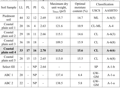
Table 1. Index Properties for Subgrade Soil and Stabilization Measures (Gabr et al., 2010) Soil Sample LL PL PI Gs

Maximum dry unit weight,

γdmax (pcf)

Optimal moisture content (%) Classification USCS AASHTO Piedmont

soil 44 32 12 2.69 115.7 14.7 ML A-6(5) Coastal

plain soil 1 20 16 4 2.63 121.6 10.9 CL-ML A-4 Coastal

plain soil 2 29 18 11 2.66 115.1 14.6 CL A-6(3) Coastal

plain soil 3 36 18 18 - 109.5 15.9 CL A-6(8)

Coastal

plain soil 4 33 17 16 2.70 113.2 15.6 CL A-6(6)

Coastal

plain soil 5 28 15 13 2.65 113.0 15.5 CL A-6(8) Select fill - - NP 2.64 - - SP A-1-b

ABC 1 20 - NP - 137.4 6.4 GW-_GM A-1-a ABC 2 22 - NP - 138.5 5.8

GW-GM A-1-a

The select fill material is a granular material without crushed stone, unlike the ABC, and was delivered from a coastal plain borrow site used by the NCDOT. The select fill material is classified as A-1-b in accordance with the AASHTO classification system.

(57)

clay minerals and by the flocculation of the soil particles. Standard Proctor compaction tests and unconfined compressive strength tests were performed for the lime-stabilized soil in order to satisfy quality control requirements.

Determination of the Stiffness and Strength Parameters

The material properties required for simulation in the large-scale tests initially were determined from the literature review, and then modified by small-scale laboratory tests, and inverse analysis. The properties to be simulated are density, stiffness, and strength parameters, such as cohesion (c) and friction (). The density () or unit weight () of each layer was obtained from the measurement of test pit samples using a nuclear gauge and sand cone device. The stiffness parameters are the elastic modulus (E) and Poisson’s ratio, and the Mohr-Coulomb strength parameters are cohesion and the friction angle. These values are required for the elastic – perfectly plastic model (the Mohr-Coulomb model) that is used in the simulation. Dilation is not considered in this study.

(58)

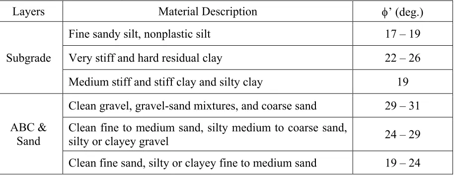
The subgrade soil used in the test pit is classified as silty clay, so the friction angle can be regarded initially as 19 degrees based on these values.

Table 2. Typical Effective Angle of Internal Friction for Unbound Granular and Subgrade Materials (NCHRP, 2004)

Layers Material Description ’ (deg.)

Subgrade

Fine sandy silt, nonplastic silt 17 – 19 Very stiff and hard residual clay 22 – 26 Medium stiff and stiff clay and silty clay 19

ABC & Sand

Clean gravel, gravel-sand mixtures, and coarse sand 29 – 31 Clean fine to medium sand, silty medium to coarse sand,

silty or clayey gravel 24 – 29 Clean fine sand, silty or clayey fine to medium sand 19 – 24

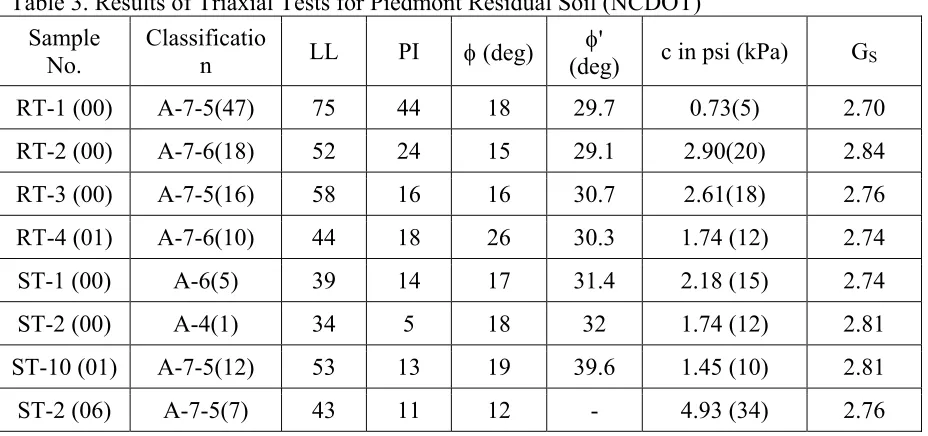
Several triaxial tests for the piedmont soft subgrade soil were conducted by the NCDOT, and the results have been provided to the project team for use in the numerical analyses, as shown in Table 3. Table 3 includes the shear strength parameters obtained from the triaxial testing. The ‘c’ and ‘GS’ in Table 3 refer to undrained shear strength and specific

gravity, respectively.

(59)

Table 3. Results of Triaxial Tests for Piedmont Residual Soil (NCDOT) Sample

No.

Classificatio

n LL PI (deg) (deg) ' c in psi (kPa) GS RT-1 (00) A-7-5(47) 75 44 18 29.7 0.73(5) 2.70 RT-2 (00) A-7-6(18) 52 24 15 29.1 2.90(20) 2.84 RT-3 (00) A-7-5(16) 58 16 16 30.7 2.61(18) 2.76 RT-4 (01) A-7-6(10) 44 18 26 30.3 1.74 (12) 2.74 ST-1 (00) A-6(5) 39 14 17 31.4 2.18 (15) 2.74 ST-2 (00) A-4(1) 34 5 18 32 1.74 (12) 2.81 ST-10 (01) A-7-5(12) 53 13 19 39.6 1.45 (10) 2.81 ST-2 (06) A-7-5(7) 43 11 12 - 4.93 (34) 2.76

Table 4. Basic Statistics of Results of Triaxial Tests for Subgrade Soil

Statistics LL PI  (deg) ' (deg) c in psi (kPa) GS

Min 34 5 12.0 29.1 0.725 (5.0) 2.70 Max 75 44 26.0 39.6 4.93 (34.0) 2.84 Mean () 50 18 17.6 31.8 2.28 (15.75) 2.77 St dev () 12.9 11.8 4.03 3.56 1.27 (8.73) 0.046

(60)

Figure 3. Comparison of effective friction angles predicted by PI values (Mitchell, 1976) and obtained from triaxial tests

As shown in Figure 3, the range of the effective friction angles predicted by the PI values is 26 to 35 degrees, and the friction angles obtained from the triaxial tests vary from 29 to 39 degrees. If the highest and lowest values are excluded, the effective friction angles plotted in the range of PI = 14 to 24 are from 29 to 32 degrees, which agrees with the empirical correlations of Mitchell (1976).

(61)

Table 5. Results of Triaxial Tests for Coastal Plain Soil

Sample No. Soil (deg) '(deg) c in psi w (%)

1 Coastal Plain 16.5 33.5 2 -

2

Mixed Coastal Plain

20.5 34.5 9.4 15.6

3 19.0 34.5 5.7 18.8

4 16.5 33.5 2 20.7

Stiffness Parameters: Elastic Modulus

(62)

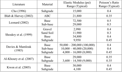
Table 6. Elastic Modulus Values and Poisson’s Ratios, as Found in the Literature

Literature Material Elastic Modulus (psi) _{Range (Typical)} _{Range (Typical)}Poisson’s Ratio Cho (1996) Subgrade 15,000 0.4 Blab & Harvey (2002) ABC 21,800 0.35

Leonard (2002) _Sub-baseBase 72,500 _29,000 0.5 _0.5

Shoukry et al. (1999)

Gravel Sand Soil Base Subgrade 2,990 11,900 34,800 9,950 0.4 0.3 0.4 0.45 Davies & Mamlouk

(1985)

Base Sub-base Subgrade

50,000 – 200,000 (100,000) 10,000 – 40,000 (20,000)

4,000 – 16,000 (8,000)

0.4 0.4 0.45 Al-Khoury et al. (2007) _SubgradeBase _{3,600 – 14,500 (9,000)}29,000 0.35 _0.35

Kwon et al. (2005) Base Subgrade

30,000 4,100

0.4 0.45

(63)

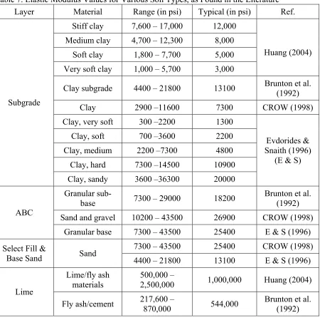
Table 7. Elastic Modulus Values for Various Soil Types, as Found in the Literature Layer Material Range (in psi) Typical (in psi) Ref.

Subgrade

Stiff clay 7,600 – 17,000 12,000

Huang (2004) Medium clay 4,700 – 12,300 8,000

Soft clay 1,800 – 7,700 5,000 Very soft clay 1,000 – 5,700 3,000

Clay subgrade 4400 – 21800 13100 Brunton et al. (1992) Clay 2900 –11600 7300 CROW (1998) Clay, very soft 300 –2200 1300

Evdorides & Snaith (1996)

(E & S) Clay, soft 700 –3600 2200

Clay, medium 2200 –7300 4800 Clay, hard 7300 –14500 10900 Clay, sandy 3600 –36300 20000

ABC

Granular

sub-base 7300 – 29000 18200 Brunton et al. (1992) Sand and gravel 10200 – 43500 26900 CROW (1998)

Granular base 7300 – 43500 25400 E & S (1996) Select Fill &

Base Sand Sand

7300 – 43500 25400 CROW (1998) 4400 – 21800 13100 E & S (1996)

Lime

Lime/fly ash materials

500,000 –

2,500,000 1,000,000 Huang (2004) Fly ash/cement 217,600 –

870,000 544,000

(64)

Figure 4. Range of elastic modulus values found in the literature (Huang, 2004; Brunton et al., 1992; CROW, 1998; Evdorides & Snaith, 1996): (a) subgrade soil layer, and (b) ABC

(65)

Table 8. Poisson’s Ratios for Various Soil Types, as Found in the Literature

Layer Material Range Typical Reference

Subgrade

Stiff clay 0.40 – 0.50 0.45 Huang (2004) Clay subgrade - 0.4 Brunton et al. ₍₁₉₉₂₎

Clay - 0.4 CROW (1998)

Clay, very soft - 0.5

Evdorides & Snaith (1996) Clay, soft - 0.45

Clay, medium - 0.35 Clay, hard - 0.1 Clay, sandy - 0.2

ABC

Untreated granular

materials 0.30 – 0.40 0.35 Huang (2004) Granular sub-base - 0.3 Brunton et al. ₍₁₉₉₂₎ Granular base - 0.35 E & S (1996)

Select Fill &

Base Sand Sand

0.30 – 0.45 0.35 Huang (2004)

- 0.35 CROW (1998)

- 0.15 E & S (1996)

Lime

Lime-stabilized

materials 0.10 – 0.25 0.20 Huang (2004) Fly ash/cement - 0.25 Brunton et al. ₍₁₉₉₂₎

(66)

stress. The range of the initial modulus values under the design stress of 70 psi for proof rolling is determined to be from 1000 to 1500 psi.

Figure 5. Determination of initial elastic modulus values from hyperbolic curves: (a) initial tangential modulus and secant modulus, and (b) relation to confining stress

Interface Properties

(67)

Kn=knw (kPa/m) (2)

Kst=ksw(n/Pa)n (kPa/m) (3)

where a normal spring coefficient is kn = 100,000, and the parameter (n) is assumed as 0.5. Based on data from pullout tests, Bauer et al. (1991) and Gabr and Hunter (1994) suggest a shear spring coefficient (ks) of 4,000 for the TN1500 geogrid (which is the same as UX1500). In this analysis, the shear spring coefficient (ks) is assumed to be the same value, i.e., 4,000.

Lime-Stabilized Soil

Standard Proctor compaction tests and unconfined compressive strength tests were performed for the lime-stabilized soil in order to satisfy quality control requirements. According to the compaction test procedure, an optimal moisture content of 16% and three days of mellowing time were applied for the coastal plain mixture, and the undrained shear strength of 50 psi was adopted for the numerical simulation.

Summary of Material Properties

(68)

elastic-perfectly plastic model were determined based on this investigation, and are presented in Table 9.

The material properties of the soils used in the large-scale tests will be used to implement the numerical simulations using the properties obtained from inverse analysis.

Table 9. Stiffness and Strength Parameters Used in the Analysis

The elastic modulus value for the select fill was assumed as 7,300 psi which was the lowest value of the range suggested by CROW (1998), and lime-stabilized soil were assumed as 500,000 psi of the range suggested by Huang (2004). For the bottom sand, the elastic modulus value was determined to be 21,000 psi, which is the highest value in the range suggested by Evdorides and Snaith (1996).

Of these material properties, the stiffness and strength parameters of the ABC, subgrade, select fill, and lime-stabilized soil affect the deformable behavior of the soft subgrade as well as the stabilized soil. Therefore, the parameters are investigated and

Material t, (lb/ft3) E (psi)  c, psi (kPa)  (deg) Sources

ABC 120 10,000 0.35 1~5 35 CROW (1998) Subgrade 114 550 ~ 1,500 0.40 5.7 19 _{Snaith (1996)}Evdorides &

Select Fill 107 7,300 0.35 2.45 34 CROW (1998) LSS 128 500,000 0.2 50 0 Huang (2004) Bottom Sand 112 21,000 0.15 0 38 Evdorides &

Snaith (1996)

(69)

(70)

INVERSE ANALYSIS

Stabilization materials typically considered for undercutting in soft subgrade soil include an ABC, select fill, lime-stabilized soil, geosynthetic reinforcements, and a combination of these materials. Except for the geosynthetic reinforcements, which are commercial products, the materials are affected by compaction energy and geological and geotechnical characteristics. It is assumed that the strength and stiffness of the test materials used in the test pit are also dependent on compaction energy and water content. By applying inverse analysis to the results of static load tests conducted in the test pit, the stiffness and strength parameters can be assessed, and the magnitude of those parameters for the stabilized soil layer can be evaluated.

Three factors are considered for the inverse analysis employed in this study: i) observation of the soil behavior, that is, the displacement and pressure measured in the subgrade soil, which are represented by the population data used in the inverse analysis algorithm; ii) the soil system in the test pit, that is, either a layered soil system or simplified homogeneous soil system; and iii) a mechanistic perspective for the simulation of the soil matrix, which is related to a constitutive model. Depending on the various combinations of these factors, the parameters (material properties) obtained from the inverse analysis will vary. For the numerical scheme, the finite difference method is used to simulate the test pit, and the Levenberg-Marquardt algorithm is adopted for backcalculation to obtain the optimized parameters.

(71)

Forward and Inverse Problems

If the physical properties of the soil system are known, and the deterministic model needed to analyze the system is also available, then the investigation can be referred to as a forward problem. As a counterpart to the forward problem, an inverse problem is solved using an assumed theoretical model that determines plausible parameters of the model using the observed data (Oliver et al., 2008). According to Oliver et al. (2008), a forward problem is considered to be well posed in that the problem has a solution, and that solution is unique and is a continuous function of the problem data (Hadamard, 1902; Oliver et al., 2008). On the other hand, some problems that arise in nature are not well posed, and are said to be ill posed. The ill posed problems refer to inverse problems.

Kubo (1992) classified the inverse problems related to field problems and their treatments. According to Kubo (1992), the governing equation in the physical domain (Ω) can be expressed as

(4)

(72)

ii) The theoretical or mathematical model (L),

iii) The boundary and initial conditions of the model (), iv) The external force acting on the domain (f), and v) Determination of the material properties (k).

The inverse analyses performed for the tests in this study are related directly to the determination of the material properties (k); thus, some geometrical boundary conditions and mathematical models are assumed in the study. The only deterministic factor is the external force (f) acting on the surface of the test pit (Ω).

Inverse Analysis of the Tests

In the geotechnical and pavement fields, the deformable behavior of a single-layer or multilayer system is commonly assessed by a mathematical model based on continuum mechanics, which is known as the finite difference method, or finite element method. The model works in a forward direction using deterministic parameters, and is used by many geotechnical engineers to predict the deformation of subsurface structures.

(73)

Figure 6. Inverse analysis scheme (after Ahn, 2009; Wang and Lytton, 1992)

(74)

Nonlinear Least Square Minimization: Levenberg-Marquardt Algorithm

The Levenberg-Marquardt algorithm is regarded as the standard method for nonlinear least-square minimization, and is applied for many inverse problems in practice (Press et al., 1992). The algorithm is defined as “the Gauss-Newton method modified by the model trust region approach” (Rus and Gallego, 2002) and is classified as a gradient method in unconstrained minimization methods (Supranata, 2006).

The nonlinear least-square problem is expressed as Eq. (5).

min

R ;

1 2

1

2RT R (5)

where R(x) is a nonlinear residual function and is defined in the domain from Rn to Rm (Rus and Gallegro, 2002). ri(x) is the n components of R(x), and commonly m≥n is assumed. The f is called a minimizer or objectives, and Marquardt (1963) used the Greek letter Φ for f.

Following a gradient descent method, the adjustment parameters (xi+1) can be

obtained by Eq. (6).

(6)

where 2

f and f are defined as follows: