Discrete Particle Model for Bedload Sediment Transport in the Surf Zone

ABSTRACT

CALANTONI, JOSEPH. Discrete Particle Model for Bedload Sediment Transport in the Surf Zone. (Under the direction of Thomas G. Drake.)

DISCRETE PARTICLE MODEL FOR BEDLOAD SEDIMENT TRANSPORT IN THE SURF ZONE

by

JOSEPH CALANTONI

A dissertation submitted to the Graduate Faculty of North Carolina State University

in partial fulfillment of the requirements for the Degree of

Doctor of Philosophy

PHYSICS

Raleigh 2002

APPROVED BY:

___________________________ ___________________________

BIOGRAPHY

ACKNOWLEDGMENTS

I would like to thank my advisor, Thomas G. Drake, for his support and guidance over the years. I also would like to thank Peter K. Haff for valuable discussions that have helped shape the works in this dissertation.

I thank Richard R. Patty for supporting my decision to pursue research in geophysics and serving on my committee. I thank Lubos Mitas for serving as a committee co-chair.

I thank Christopher S. Thaxton for years of insightful discussions and for providing useful revisions of Chapters 4 and 5. I thank David M. Pierson for his tireless efforts to keep my computers running and secure.

TABLE OF CONTENTS

LIST OF FIGURES ... vii

Chapter 1...1

1.1. Bedload Transport ...3

1.1.1. Sheet Flow Transport in the Surf Zone ...4

Chapter 2...6

2.1. Introduction...6

2.2. Simulation Models ...7

2.2.1. Particle Model...7

2.2.2. Discrete- fluid model ...8

2.2.3. Comparisons with King's Experiments...10

2.2.4. Waveforms...10

2.3. Energetics-Based Models ...12

2.4. Results...13

2.5. Conclusion...13

Chapter 3...16

3.1. Introduction...16

3.1.1. Transport Models ...17

3.1.2. Sheet Flow Transport...19

3.2. Description of Simulations ...20

3.2.1. Particle-Particle Interactions...22

3.2.2. Discrete Fluid Model ...23

3.2.3. Particle Fluid Interactions ...26

3.3. Sheet Flow Simulations ...28

3.3.1. Description of Simulations ...28

3.3.2. Comparison With Experiment ...28

3.3.3. Simulation Sensitivity to Parameter Variation...29

3.4. Simulation of Surf Zone Conditions ...37

3.4.1. Simulated Waveforms ...37

3.4.2. Role of Acceleration in Unsteady Bedload Transport...37

3.5. Conclusions ...44

Chapter 4...45

4.1. Introduction...45

4.1.1. Bedload Transport Models ...46

4.2. Discrete Particle Model ...49

4.2.1. Model Assumptions ...49

4.3.1. Beds Sloping Transverse to the Flow Direction...53

4.3.2. Beds Sloping Along the Flow Direction...55

4.4. Discussion...61

4.4.1. Slopes Transverse to Flow Direction...62

4.4.2. Slopes Along Flow Direction ...62

4.4.3. Dependence of the Net Transport Rate on Wave Period ...63

4.4.4. Effects of Particle Shape on Bedload Transport ...65

4.4.5. A New Formulation for Bedload Transport...65

4.5. Conclusions ...70

Chapter 5...72

5.1. Introduction...72

5.2. The Composite Particle ...73

5.2.1. Volume Calculation...73

5.2.2. The Principle Moments of Inertia ...74

5.2.3. The z-coordinate of the CM...76

5.2.4. The Principle Moments of Inertia About the CM...77

5.3. Modifications to Code ...78

5.3.1. Contact Detection and Forces ...78

5.3.2. Rotational Motion of the Composite Particle ...79

5.4. Quantifying the Shape of Natural Particles ...79

5.5. Simulations with Composite Particles ...80

5.5.1. Simulation Results ...83

5.6. Discussion of Application to Bedload Transport Modeling ...85

5.6.1. Drag Force ...85

5.6.2. Settling Velocity...86

5.7. Conclusions ...86

LIST OF FIGURES

Figure 2.1. Snapshot from a typical simulation. ...9

Figure 2.2. Time series of near-bed flow velocity (thin line), flow acceleration (heavy line) and bedload flux (x) for transport over a horizontal planar bed for waveform parameter

0

φ = (top), φ π= 4 (middle), and φ π= 2 (bottom). ...11

Figure 2.3. Time-averaged net bedload flux versus tangent of the bed slope for three

waveforms (closed circle, φ =0; open square, φ π= 4; and closed triangle, φ π= 2).15

Figure 3.1. Schematic picture of discrete particle simulation. Sand grains are modeled as frictional spheres having the density of quartz (ρ =2650 kg m-3) and a distribution of

sizes corresponding to experiments by King [1991]...24

Figure 3.2. Grain-size distribution for King [1991] flow tunnel experiments sharply peaked

about a mean grain size of 1.1 mm. ...30

Figure 3.3. Comparison of predicted bedload transport rates from simulations with physical experiments conducted by King [1991] in an oscillatory flow tunnel using natural quartz

sand with the distribution of sizes shown in Figure 3.2. ...31

Figure 3.4. Time-averaged bedload transport rate, weakly dependent on the bed

concentration Nz, which fixes the origin for determination of the mixing length. ...35

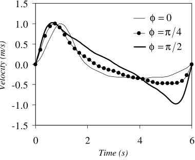
Figure 3.5. Variation in waveform for φ =0, π 4, and π 2 for 6-s wave periods having a

maximum fluid velocity of 1 m s-1. ...38

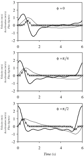
Figure 3.6. Time series of near-bed fluid velocity (thin line), acceleration (thick line) and

bedload flux (circles) from simulated waveforms having φ =0, π 4, and π 2...40

Figure 3.7. Total impulse-generated transport, increasing linearly with impulse above a

minimum impulse of ∼1 m s-1...41

Figure 3.8. (top) Bedload flux varying approximately linearly with u3 , except for strongly asymmetric waves having φ π= 2 and 3

u equal to zero...43

Figure 4.1. (top) The flow is perpendicular to the local slope in this case. The transverse flux will always be down the local slope regardless of the sign of α. ...48

Figure 4.2. (top) Shows comparison with King’s [1991] data taken in an oscillatory flow

tunnel for a horizontal bed. ...51

Figure 4.3. As the waveform parameter, φ, is varied from 0 to π 2 the shape of the velocity time series near the bed goes from skewed to asymmetric, grossly representing the range of conditions from shoaling to broken waves with the φ π= 2 waveform representing

the sawtooth characteristic of surf zone bores. ...52

Figure 4.4. Monochromatic waves with 6 s periods, maximum velocity amplitudes ranging

Figure 4.5. Plotted above is the net bedload flux (normalized by a constant) versus the

tangent of the bed slope, β, along the flow direction. ...57

Figure 4.6. (top) Time series for the sawtooth waveform (velocity skewness = 0) and (bottom) the skewed waveform (velocity skewness = 1.2) of the fluid velocity and

bedload flux. ...59

Figure 4.7. The parameterization of bedload flux previously proposed for 6 s period waves under a range of unsteady flow conditions does appear to offer some reasonable predictions of the net flux when tested against simulation results for waves of 3 s and 12 s periods with all other wave parameters (and grain size) being held constant...64

Figure 5.1. Shown is a composite particle in plan view (maximum projected area). ...75

Figure 5.2. The physical limits of the composite particle range from the (a) sphere to the (b)

perfect dumbbell. ...81

Figure 5.3. The ratio, R2:R1=0.5, is constant for all the particles shown here. ...82

Figure 5.4. Each p is the average critical angle of 10 successive simulations with one

Chapter 1

Introduction

Transport of sand and coarser sediments by waves and currents in the nearshore environment is characterized by two dominant modes: bedload transport, in which grains collide, slide, bounce, and roll in close proximity to the bed, and suspended load, in which grains are lifted from the bed by fluid turbulence and suspended within the water column. This work focuses exclusively on a particular bedload transport phenomenon called sheet flow, which occurs under a limited but not atypical set of conditions observed in the surf zone during storms. Following a short introductory discussion of extant theories for bedload transport and sheet flow in particular, the remainder of the dissertation comprises a series of chapters either already published or soon-to-be submitted for publication. The chapters are presented in roughly chronological order.

Chapter 2 uses a discrete-particle modeling approach to address the concept of a local equilibrium beach slope [Calantoni and Drake, 1999]. The simulation predicts an

equilibrium beach slope under conditions where the often-used transport model of Bailard and Inman [1981] is unable to make a prediction, revealing a shortcoming of their approach that is addressed in the following chapters.

Chapter 3 provides a detailed description of the discrete particle model, details the shortcomings of the energetics approach to bedload transport, and proposes an additional term in the Bailard [1981] bedload formula that accounts for effects of fluid acceleration in the transport process. A physical explanation for the additional term is presented and simulations are used to determine constants in the new theory.

provided that the critical threshold for motion is surpassed. The goal is to provide a vectorial bedload transport relation for surf zone transport that accounts for the effects of gravity on an arbitrarily oriented bed to the direction of the fluid forcing.

Chapter 5 introduces a significant enhancement of the discrete particle model that allows simulations to incorporate non-spherical particles, which are constructed from pairs of overlapping spheres which are hereafter referred to as composite particles. A suite of

simulations demonstrates that varying the shape of composite particles in a systematic way allows quantitative prediction of the range of angles of repose observed in physical

experiments for a variety of particle shapes and frictional properties.

1.1. Bedload Transport

Early work on bedload transport focused on steady flows characteristic of fluvial environments [Meyer-Peter and Müller, 1948; Einstein, 1950; Bagnold, 1966]. Bailard [1981] and Bowen [1980] independently constructed so-called energetics models for

sediment transport in the surf zone based in part on Bagnold’s theory [1966] for steady flows in rivers. For surf zone flows dominated by pervasive offshore flow, the Bagnold-Bowen-Bailard models (hereafter BBB) have demonstrated predictive skill [Thornton et al., 1996; Gallagher et al., 1998]. Unfortunately, several of the parameters in the BBB theories are difficult to evaluate, even with direct observations of bedload motion. In the surf zone,

to provide a physically based model for bedload transport with no or few free parameters that can be tested with available field observations.

An alternative approach to modeling bedload transport based on kinetic theories for collisional grain flow has been proposed by Jenkins and Hanes [1998]. Their continuum approach to modeling granular flow treats the particle concentration in bedload as a

continuous field [Jenkins and Savage, 1983; Haff, 1983]. Hsu [2002] generated a two-phase flow approach for bedload transport based on a kinetic theory approach and turbulent mixture theory. An informal, preliminary comparison of results from Hsu’s model and the model used here at a recent meeting showed a number of qualitatively similar predictions, which may form the basis for collaborative work in the near future.

1.1.1. Sheet Flow Transport in the Surf Zone

Chapter 2

Discrete-Particle Model for Bedload

Transport: Implications for the Concept of

Local Equilibrium Bed Slope in Oscillatory

Flows

This chapter was co-authored by Thomas G. Drake and published in a similar form in the Proceedings of the International Association of Hydraulic Research on River, Coastal and Estuarine Morphodynamics, held September 6-10, 1999, in Genoa, Italy.

2.1. Introduction

A variety of sloping planar sediment surfaces typically occur in the surf zone, from the offshore-sloping swash zone to bed form surfaces sloping in all directions to bars having both onshore- and offshore-directed slopes. It is exceedingly difficult to make field

conditions, and to address the implications of simulation predictions for the concept of a local equilibrium bed slope. The local equilibrium bed slope is that slope for which there is a local balance in transport, such that the onshore flux of sediment equals the offshore flux [e.g., Inman and Bagnold, 1963]. This paper does not address the generation of an equilibrium beach profile, which has been the subject of extensive study [e.g., Dean, 1977; Inman et al., 1993, among many others].

Our simulations raise questions about the validity of the local equilibrium bed slope concept in many natural situations of interest; in particular, our simulations predict a slope of several degrees for certain commonly observed nearshore waveforms, whereas existing

energetics-based models [e.g., Bagnold, 1963, 1966; Bowen, 1980; Bailard and Inman, 1981] predict a local equilibrium bed slope of zero.

2.2. Simulation Models

Discrete-particle computer simulation models based on molecular-dynamics-like models for flowing granular materials [Drake and Walton, 1995] are used to simulate bedload transport of grains having nearly arbitrary diameter, density, elastic and frictional properties. Bedload transport rates predicted with the present model [Calantoni and Drake, 1998a;b] compare favorably with available experimental data for bedload transport of coarse sand in an oscillatory flow tunnel [King, 1991].

2.2.1. Particle Model

consist of particle-particle forces; particle-fluid forces; and pressure-gradient and gravitational body forces. Normal and tangential forces generated between contacting

spheres are based on approximations [Walton and Braun, 1986a;b] to theoretical models for identical, homogeneous Hertzian elastic spheres developed by Mindlin and Deresiewicz [1953]. Fluid-particle interactions consist of buoyancy, drag and added mass forces. The coefficients of drag and added mass depend on the volume concentration of particles in the fluid.

2.2.2. Discrete-fluid model

and rotation at the opposite side of the volume. The lower boundary of the calculational volume is a smooth plane with several fixed spheres to prevent wholesale sliding of the granular assemblage. The initial particle configuration is generated by gravitational settling of particles from a regular lattice into the calculational volume. Although larger particles settle more rapidly than smaller ones, the relatively high concentration effectively hinders size sorting during the settling process.

2.2.3. Comparisons with King's Experiments

King's [1991] oscillatory flow tunnel experiments using 1.1 mm mean diameter quartz sand in fresh water provide mean total sediment transport rates for half-cycle oscillatory flows under sinuosoidal and other waveforms in both horizontal and tilted-bed configurations. The model consistently reproduces results obtained by King to within about 20% [Calantoni and Drake, 1998a,b]. Our simulation approach is untested, at present, for finer-grained particles used in a number of other experiments.

2.2.4. Waveforms

The three different waveforms simulated are generated using a truncated Fourier series expansion for a sawtooth wave

( )

(

(

)

)

5 1

1

, o 2 kcos 1

k

u t φ u − k tω k φ

=

=

∑

Figure 2.2. Time series of near-bed flow velocity (thin line), flow acceleration (heavy line) and bedload flux (x) for transport over a horizontal planar bed for waveform parameter φ =0

(top), φ π= 4 (middle), and φ π= 2 (bottom). -2 -1 0 1 2 3

0 2 4 6

Velocity (m/s) Acceleration (m/s/s) Flux (kg/m/s) -2 -1 0 1 2 3

0 2 4 6

Velocity (m/s) Acceleration (m/s/s) Flux (kg/m/s) Time (s) 0 φ = 4 φ π= 2 φ π= -2 -1 0 1 2 3

0 2 4 6

Velocity (m/s)

Acceleration (m/s/s)

acceleration and bedload flux for each of the three simulated waveforms is shown in Figure 2.2.

2.3. Energetics-Based Models

Inman and Bagnold [1963] recognized the effect of asymmetrical velocity distributions and presented the following model for the equilibrium beach slope

1 tan tan

1

r

c c β = φ _ − _

+

  (2.2)

where c is defined as the ratio of the amount of energy dissipated during the offshore sediment flow divided by the amount of energy dissipated during the onshore sediment flow and tanφ_r is about 0.63 [Bagnold, 1956]. Bailard and Inman [1981] refined this relationship to the form

3

3

tan tan r

u

u

β = φ (2.3)

where u is the oscillatory flow velocity and angle brackets indicate time averaging. While Bailard and Inman [1981] explicitly assume tanβ=tanφ_r in their derivation of equation (2.3), that assumption is often ignored by other workers.

Equation (2.3) predicts β = 25º, 20º and 0º, respectively, for waveform parameter

0

2.4. Results

Simulations were conducted for a range of bed slopes from –10º to +10º for each of the three waveforms (Figure 2.3). Slopes greater than zero correspond to wave propagation in the uphill direction. Flux for each simulation is time-averaged over one full wave period and has been normalized by the simulated flux for the waveform parameter φ =0 at zero slope. The simulation was run for at least two full wave periods and the data from the first period discarded because of transient sorting effects associated with the initiation of a run. The transport rate varies linearly with the tangent of the bed slope, β, for each of the three waveforms for slopes of about –7º to +7º. Only the sawtooth waveform exhibits a local equilibrium beach slope of about 7º; the curves for the other waveforms do not cross the abscissa for the range of slopes simulated to date. For slopes having magnitudes greater than about 7º the dependence of the transport rate on tanβ departs from linearity, and

preliminary simulations indicate that the dependence is decidedly nonlinear for slopes having magnitude greater than about 10º. Further simulations are underway to explore this nonlinear dependence.

2.5. Conclusion

0.2

0.1

0.0

-0.1

-0.2

-1

0

1

2

3

4

Tangent of the bed slope

Normalized flux

Wave propagation downhill Wave propagation uphill

Figure 2.3. Time-averaged net bedload flux versus tangent of the bed slope for three

Chapter 3

Discrete Particle Model for Sheet Flow

Sediment Transport in the Nearshore

I co-authored this chapter with Thomas G. Drake and it was published in a slightly different form in the Journal of Geophysical Research, Oceans, volume 106(C9), pages 19,859-19,868, on September 15, 2001.

3.1. Introduction

3.1.1. Transport Models

Nearshore bedload transport models are not robust. Energetics models, based on Bagnold's [1966] theory for bedload transport in unidirectional flows, have been extended to unsteady nearshore flows by relating the sediment transport rate to moments of the near-bed fluid velocity [Bowen, 1980; Bailard, 1981]. Application of the Bagnold/Bowen/Bailard (BBB) models to field measurements predicts storm-generated offshore migration of bars at Duck, North Carolina, with some skill [Thornton et al., 1996; Gallagher et al., 1998]. Fluid motion during storms at Duck is dominated by strong offshore-directed mean currents

(although sizable longshore currents are measured in the field, only the cross-shore currents are used in one-dimensional bathymetric models). These currents roughly conform to assumptions used by Bagnold to derive the energetics model. During relatively quiescent conditions, on the other hand, when oscillatory flow velocities are much greater than mean flows, BBB models typically fail to predict gradual onshore bar migration [Gallagher et al., 1998]. We and others have suggested [Calantoni and Drake, 1998; Elgar et al., 2001] that transport depends in some measure on the fluid acceleration in addition to fluid velocity. The primary objectives of this study are to indicate the role of fluid accelerations in nearshore bedload transport and to suggest modifications to the BBB models suitable for application to field measurements of nearshore fluid motion. We use discrete particle computer simulations to study the bedload motion of individual sediment particles under a restricted but highly relevant range of nearshore flow conditions: intense, collision-dominated bedload transport of coarse sand grains.

considerable body of observation and theory support the general form of Bagnold's transport relationship for unidirectional flows. Bailard’s [1981] time-averaged bedload sediment flux equation, expressed as mass sediment transport per unit width per unit time (analogous to Thornton et al. [1996]), is given as

2 2 tan 3

( ) ( ) ( ) ( )

( ) tan tan

s b

f s

q c t u t t u t

g

ρ ε β

ρ

ρ ρ φ  φ 

= _{− } + + _

 u % u u , (3.1)

where q is the bedload flux, ρ and ρ_s are fluid and sediment densities, g is gravitational acceleration, u(t) is the time-varying velocity, tanβ is the bed slope, φ is the angle of internal friction, c_f is the friction coefficient, ε_b is the bedload efficiency, overbar indicates mean velocity, tilde indicates oscillatory velocity, and angle brackets indicate time averaging. For cross-shore transport of coarse bedload on a horizontal bed due to oscillatory flow, ignoring transport due to mean currents, Bailard’s equation reduces to

3

( )

( - ) tan

s b

f s

q c u t

g

ρ ε

ρ

ρ ρ φ

= (3.2)

Here we consider a BBB-like model having an additional term depending on an unknown function ƒ of the near-bed fluid acceleration, a:

3

( )

q =k u + f a (3.3)

3.1.2. Sheet Flow Transport

Large surface gravity waves in shallow water generate intense bedload transport commonly called sheet flow transport [Dingler and Inman, 1976], which is thought to be a primary agent in nearshore bathymetric and sedimentologic evolution. Available field [e.g.,

Dingler and Inman, 1976; Conley and Inman, 1992] and laboratory [e.g., Wilson, 1987; King, 1991; Ribberink and Al-Salem, 1994; Sumer et al., 1996] observations of sheet flow indicate that bedload motion is confined to a nearly horizontal layer of moving grains up to a few

centimeters in thickness with a distinct upper surface. Under sheet flow conditions the bed remains nominally planar and thus roughly corresponds to the upper flow regime in

unidirectional flows [e.g., Gilbert, 1914; Middleton and Southard, 1984]. The absence of ripples and other bed topography during sheet flow simplifies description of the bulk fluid motion to that of a two-phase turbulent flow. Hanes and Bowen [1985], Hanes [1986], Nadaoka and Yagi [1990], and Jenkins and Hanes [1992, 1993, 1998] present continuum theories for steady, collision-dominated sediment transport founded on the work of Bagnold [1954]. The focus of this paper is on the widely used energetics models and their application to unsteady flows not addressed by the continuum theories.

[1998] used a three-dimensional discrete particle model to address effects of fluid velocity fluctuations in unidirectional flows.

Section 3.2 describes each element of the particle and fluid models employed in the simulations. Section 3.3.3 describes the sensitivity of the model to several parameters. The remainder of the paper describes a comparison of simulation results with several physical experiments and presents a detailed particle-scale picture of oscillatory bedload transport phenomena. Section 3.4.2 proposes a physical mechanism for the inclusion of an acceleration term in the oscillatory bedload transport equation of Bailard and describes a new quasi-empirical formula for sheet flow bedload transport under oscillatory flow that uses fluid motion quantities commonly measured in the field.

3.2. Description of Simulations

collective particle motion that occurs when fluid stresses exceed the shear strength of the granular bed. The approach explicitly de-emphasizes the short initial and final stages of grain motion over a relatively immobile bed and hypothesizes that grain-grain interactions

dominate the stresses within a high-concentration granular fluid. Such interactions begin to dominate over fluid interactions when the solids volume concentration exceeds about 8% [Bagnold, 1954].

One commonly used measure of the relative importance of interstitial fluid effects in grain-fluid systems is the Bagnold number [e.g., Hanes and Bowen, 1985]

1

2 ₂ 1

s du B D dz ρ λ µ− = (3.4)

where D is the grain diameter, du/dz is the velocity gradient, µ is the dynamic fluid viscosity, and the linear concentration λ [Bagnold, 1954] is

(

)

1 ₃

0 1

N N

λ− _{= − (3.5)}

where N₀ ≈0.65 is the maximum value of the solids volume concentration N. For values of 450

B≥ , Bagnold’s experiments indicate that grain-grain interactions dominate viscous effects. The simulations presented here address such collision-dominated granular fluid flows.

Using Dingler and Inman’s [1976] field criterion for incipient sheet flow,

2 max

240

( s )

U gD ρ ρ ρ

Θ = ₋ ≥ , (3.6)

maximum orbital velocities Umax on the order of 1 m s

-1

simplifies the treatment of particle-fluid interactions because it justifies neglecting lubrication forces between particles.

In the discrete particle model, velocities and positions of discrete spherical particles are obtained by integrating Newton’s equations of motion at small time steps, and an

analogous set of equations for the torques on the spheres is solved to provide their spins and orientations. Forces are generated by direct particle-particle contact; by such fluid-particle interactions as buoyancy, drag, and added mass effects; and by pressure gradients and gravitational forces. An eddy-viscosity-based model describing interactions between discrete fluid elements completes a self-consistent physical description of the bedload transport process.

3.2.1. Particle-Particle Interactions

Normal and tangential forces between contacting spheres are based on approximations [Walton and Braun, 1986a, 1986b; Drake and Walton, 1995] to theoretical models for identical, homogeneous Hertzian elastic spheres developed by Mindlin and Deresiewicz [1953]. The magnitude of the normal force Fn between contacting particles is given by

For loading (approaching particles)

1

=

n

F k a (3.7)

For unloading (receding particles)

(

)

2 0 3

max[ , ]

n

F = k a a− k a (3.8)

(

)

1 2

e= k k (3.9)

The tangential force Ft, described in detail by Drake and Walton [1995], is

min( , )

t t n

F = kds µ_φF , (3.10)

where k_t is the tangential stiffness, ds is the tangential displacement at the contact point, µ_φ is the friction coefficient (no distinction is made here between sliding and static friction), and the sign of F_t opposes relative motion of the spheres at the point of contact.

The particular models used here were tested and refined by comparisons of simulations with physical experiments of dry granular flows using homogeneous plastic

spheres [Drake and Walton, 1995; Foerster et al., 1994]. Bedload transport simulations using the same plastic spheres compare favorably with physical experiments [Drake et al., 1991] and are insensitive to variations in the particle stiffnesses and friction coefficient, a feature also noted by Jiang and Haff [1993]. Interparticle force models used in discrete particle simulations are the subject of considerable research. A discussion of potential pitfalls (primarily associated with velocity-dependent damping models not used here) is given by Luding et al. [1994]. Natural sand and gravel particles are neither spherical nor

homogeneous, and whereas our simulations are robust with respect to the details of particle-particle interactions, we are also pursuing studies of nonspherical, inhomogeneous particle-particles (see Chapter 5) that may explain subtle features of the simulations noted in section 3.3.

3.2.2. Discrete Fluid Model

Figure 3.1. Schematic picture of discrete particle simulation. Sand grains are modeled as frictional spheres having the density of quartz (ρ =2650 kg m-3) and a distribution of sizes corresponding to experiments by King [1991]. Grains larger than 1.5 mm diameter are colored gold to aid visualization of particle sorting processes. Fluid motion is modeled using discrete slabs constrained to move parallel to the bed. Length of the slabs is proportional to fluid velocity. Periodic boundaries are used in both the cross-shore and alongshore

within them. Linear wave theory is used to determine the fluid pressure gradients at the bed [Guza and Thornton, 1980]. Streamwise fluid pressure gradients within the volume are approximately constant because the dimensions of the simulation volume are small and thus closely resemble those in a laboratory flow tunnel. The layers in the stack exchange

momentum via an eddy viscosity determined from a mixing length model. Each fluid layer exerts drag, added mass, and pressure gradient forces on particles embedded within it. Particles exert equal and opposite forces on the fluid layers, thus fully coupling fluid and sediment motion. Turbulence is implicit in a mixing length approach, and thus the fluid velocity within each layer is constant and explicitly excludes particle-generated wakes or other grain-scale turbulent fluid motions. The layer model inherently suppresses development of such bed features as ripples. However, under sheet flow conditions, local bed topography is planar.

The choice of mixing length model is largely guided by the desire to minimize simulation complexity and is an area for improvement. A mixing length model provides a simple mechanistic picture of the fluid-grain mixing process, despite its well-known limitations [e.g., Tennekes and Lumley, 1972]. The effective viscosity υ_eff that mediates momentum transport between fluid layers is the maximum of the fluid kinematic viscosity υ and an eddy viscosity:

2

max( , )

eff

u l

z ∂

υ = _{υ ρ ∂} , (3.11)

where l is the mixing length. The mixing length is the vertical distance upward from an origin z0 taken where the volume concentration of particles Nz exceeds a fixed value,

3.3.3.3). Defining the origin of the mixing length is problematic, as the problem is not only geometrical. For example, the nominal bed level defined by fluid flow considerations, such as the origin of a logarithmic velocity profile, is not necessarily the same as that defined by particle motion considerations, such as the average elevation of the tops of surface particles [Drake et al., 1988].

The mixing length model enforces a law-of-the-wall velocity profile, except in the region of bedload motion and immediately above it, where momentum extracted by particles causes significant deviations from a particle-free velocity profile. Exploratory simulations using alternative forms for the effective viscosity [e.g., Trowbridge and Madsen, 1984a, 1984b] proved insensitive to the choice of model.

3.2.3. Particle Fluid Interactions

The equation of motion for sediment particles [Madsen, 1991] is

( ) f f

s s

s s m

D D

d d

V gV V c V

dt Dt Dt dt

ρ = ρ ρ− +ρ + ρ _ − _

 

u u

u u

1

(

)

2ρC Ad f s f s φ

+ u −u u −u +F , (3.12)

where u_s and u_f are the sediment and fluid velocities, V and A are the volume and projected area, respectively, of the sediment grain, Cd and cm are the drag and added mass coefficients,

flows. However, the turbulent structure in such fully developed boundary layer flows differs significantly from that in oscillatory boundary layers. Finally, although particle rotations are generated by frictional particle contacts, no fluid drag forces resist rotational motion in the simulation.

The first four terms on the right-hand side of (3.12) represent the buoyancy force, the fluid acceleration force, the added mass force, and the drag force. Jiang and Haff [1993], following Landau and Lifshitz [1987], accounted for the added mass force by increasing the particle mass by 20%, appropriate for quartz-density particles in water. Here the coefficient of added mass, cm, is 0.5 [Batchelor, 1967]. The drag coefficient Cd depends on the

instantaneous value of the particle Reynolds number Re_s =U D_rel υ as follows:

1

1 ₂

24 4 0.4

d s s

C = Re− + Re − + , (3.13)

where U_rel is the magnitude of the relative velocity between sediment and fluid. Experiments to determine Cd for fixed grains in a steady, uniform unidirectional flow by Schmeeckle

[1998] indicate that the still water coefficient described by (3.13) underestimates the true drag coefficient by as much as 50% or more. Engineering studies of fluidized bed

phenomena indicate that both cm and Cd may depend strongly on local volume concentration

3.3. Sheet Flow Simulations

Simulations of oscillatory sheet flow are compared with the limited data available from physical experiments. Additional simulations explore a small subset of the parameter space to determine simulation sensitivity to variations in parameters, particularly those that are poorly constrained by theory or observation. A final set of simulations explores waveform effects and critically tests BBB models with the results used to propose an additional term for the BBB equations.

3.3.1. Description of Simulations

Figure 3.1 is a schematic diagram of the simulations. Periodic boundaries are used in both the cross-shore and alongshore directions, and thus particles exiting any side of the calculational volume are reintroduced with identical velocity and rotation at the opposite side of the volume. The lower boundary of the calculational volume is a smooth plane to which several spheres are fixed to prevent wholesale sliding of the granular assemblage, and the thickness of the granular bed is chosen such that the maximum depth of motion never reaches the fixed bed spheres. The initial particle configuration for each simulation is generated by gravitational settling of particles from a regular lattice into the calculational volume. Although larger particles settle more rapidly than smaller ones, the relatively high concentration effectively hinders size sorting during the settling process.

3.3.2. Comparison With Experiment

particles. King’s [1991] flow tunnel experiments using 1.1-mm mean diameter quartz sand (Figure 3.2) provide sediment transport rates for half-cycle oscillatory flows under

sinuosoidal and other waveforms in both horizontal and tilted bed configurations. Although King’s data do not include all the information necessary to calculate the Bagnold number, conservative estimates of the quantities in (3.4) for a number of King's experimental runs greatly exceed Bagnold’s criterion, except at the initiation and cessation of motion. Simulated transport rates for half-period sine waves having periods and maximum fluid velocities identical to King's experiments are compared in Figure 3.3. For maximum fluid velocities <1.1 m s-1 the simulated rates are within 20% of King's measured rates. For maximum fluid velocities >1.1 m s-1, agreement is within 25%. Simulation transport rates are mean rates calculated from at least three half periods, and transport rates during the first half period of a simulation are excluded due to transient size sorting of the initial particle

configuration.

3.3.3. Simulation Sensitivity to Parameter Variation

Several parameters must be specified for simulation of sheet flow, including several describing properties of solid particles and discrete fluid layers. This section discusses simulation sensitivity to these parameters and physical reasoning for specifying parameters that are poorly constrained by theory and/or physical experiment.

3.3.3.1. Particle Parameters

Figure 3.2. Grain-size distribution for King [1991] flow tunnel experiments sharply peaked about a mean grain size of 1.1 mm.

Diameter (mm)

0.5

0

10

20

30

40

50

1

2

Typical simulation

uses 1600 particles

D

= 1.1 mm

Figure 3.3. Comparison of predicted bedload transport rates from simulations with physical experiments conducted by King [1991] in an oscillatory flow tunnel using natural quartz sand with the distribution of sizes shown in Figure 3.2. (top) Bedload flux produced by maximum free stream fluid velocities ranging from just above that required for incipient motion to nearly 1.2 m s-1. (bottom) Bedload flux versus bed slope for maximum free stream fluid velocity of 1 m s-1.

1.2

1.0

0.8

0.0

0.1

0.2

0.3

0.4

Maximum velocity

(

m s

₎

(

kg

m

-1

s

-1

)

Bed load flux

10

5

0

-5

-10

0.0

0.2

0.4

0.6

Bed slope (degrees)

(

kg

m

-1

s

-1

)

Bed load flux

and friction coefficient, several of which were varied while holding others fixed. While the initiation and cessation of sediment motion may be described only poorly in simulations using spherical particles, physical experiments [Drake et al., 1991] imply that the bulk properties of a thick bedload layer are largely independent of particle shape. Description of the parameters and simulation sensitivity to parameter variations are reported below. Although some of the parameters for natural sediments are poorly known, sensitivities are small. We define baseline simulations as those simulations in which the stiffness

5 -1

1 10 N m

k = , the normal coefficient of restitution e = 0.6, and the coefficient of friction

1

µ= .

Particle Stiffness.

The stiffness of pure quartz spheres can be calculated from elastic constants, but stiffness measurements for individual clasts in natural sediments comprising single mineral grains or aggregates of them are exceedingly difficult. Thus the stiffness k1 in discrete particle

simulations is essentially a free parameter, constrained by physical and pragmatic

diameter, and typical overlaps were much less than 0.5%. The duration δt of a particle-particle collision in the absence of fluid forces is proportional to the normal coefficient of restitution, e, and inversely proportional to k₁1 2. In practice, δt was typically 4

4 10 s× −

: in

the simulations, using k₁ =10 N m5 -1. Restitution Coefficient.

The normal coefficient of restitution for irregular natural particles varies considerably depending on the particle and collision geometries. Tabletop experiments (T. G. Drake, unpublished data, 1996) using natural sand and gravel particles indicate a range of e from >0.8 to <0.1, typically in the range 0.1 to 0.5. Recent experiments by Schmeeckle [1998] also indicate coefficients of restitution for immersed particle collisions in a similar range. Bedload transport rates in the simulations are insensitive to the restitution coefficient. Differences in instantaneous transport rates for e=0.15, 0.3, and 0.6 are statistically insignificant. Baseline simulations use e=0.6.

Friction Coefficient.

Sensitivity to variations in friction coefficient µ is small, provided that µ is nonzero. The presence of surface asperities on natural rough particles typically prevents relative tangential velocity at particle contacts, and adopting µ≥1 for geometrically smooth spheres effectively approximates the observed rotational motion of natural particles [e.g., Drake et al., 1988]. Baseline simulations use µ =1.

3.3.3.2. Fluid Layer Parameters

than Dx). Simulations are insensitive to the number of fluid layers, provided that at least some

layers always remain grain-free during the simulation. Layer thickness was chosen to resolve sufficient particle-scale detail in the bedload layers and to minimize statistical uncertainties in simulation quantities. In particular, layers thinner than the mean particle diameter often have too few particles for statisically significant determination of layer concentration. In contrast, simulations using fluid layers thicker than about one or two mean particle diameters often exhibit discontinuities in transport rates and also grossly mispredict initiation of particle motion. In practice, the typical layer thickness was 1 mm, which also ensured that each particle occupies volume in, at most, two layers.

3.3.3.3. Nominal Bed Concentration

The free parameter Nz is symptomatic of the uneasy but requisite union of granular

and fluid mechanics at the sediment-water interface. The choice of Nz = 0.4 is justified

heuristically as follows. At concentrations exceeding 0.4 the mean free path between particles is less than half a particle in diameter and vertical exchange of grains within the sheet flow layer is diminished greatly. Bulk transport of fluid momentum by eddies is likewise inhibited and is effectively limited to scales larger than the thickness of the discretized fluid layers. Perhaps surprisingly, the simulations are rather insensitive to variations in Nz (Figure 3.4).

3.3.3.4. Effect of Computational Domain Size

Figure 3.4. Time-averaged bedload transport rate, weakly dependent on the bed concentration Nz, which fixes the origin for determination of the mixing length. Circles indicate variation of Nz for one half-period (i.e., onshore) sinusoidal oscillatory flow having a period of 6 s and maximum free stream velocity of 1 m s-1. Triangles indicate variation in net flux for a full 6-s period sawtooth oscillatory flow having the same maximum free stream velocity of 1 m s-1. Weak dependence of transport rate on Nz for 0.2 < Nz < 0.5 is observed for all simulated flows.

Bed concentration N

_z

Bed load flux (kg m

-1

s

-1

)

0.6

0.4

0.2

0.0

0.0

0.2

0.4

0.6

0.8

sine wave

descriptors as transport rate to be largely insensitive to variations in computational domain size, provided the domain exceeded certain minimum dimensions. Similiar testing of the present simulation indicates that a cross-stream domain dimension of only about five particle diameters is sufficient. The height or thickness of the computational domain should be at least twice the thickness of the bedload layer, with a streamwise domain dimension roughly equal to the domain height. Dependence of transport rates on domain dimensions is small; a worst-case disparity of 13% increase in transport rate occurred in a simulation for which the streamwise domain dimension was doubled from the baseline value. Such variability is small relative to natural fluctuations in transport rates and fluid forcing.

3.3.3.5. Computational Issues

3.4. Simulation of Surf Zone Conditions

3.4.1. Simulated Waveforms

A suite of simulations using five different waveforms having a constant period T=6 s and maximum fluid velocities of 0.5, 0.75, 1.0, 1.25, and 1.5 m s-1 was used to explore the effects of wave shape on bedload transport. As expected, simulated waveforms producing 0.5 m s-1 maximum fluid velocities transport essentially no sediment. The time-varying pressure

gradient force F t( ) exerted on the slabs and grains in the stack is proportional to

[

]

4

0

1

( ) sin ( 1) 2i

i

F t i ωt iφ

=

∝

∑

where ω=2π T and φ is the waveform parameter. The waveform parameter corresponds to the biphase [e.g., Elgar and Guza, 1986; Elgar and Chandran, 1993]. Figure 3.5 shows near-bed fluid velocity time series for waveforms having φ =0, π 4, and π 2 (waveforms

having φ π= 8 and 3π 8 were also simulated). Such variation in φ encompasses a wide qualitative range of shoaling and broken waves. We also simulated waveforms having

2

φ π> , but such waves are not typical of natural surf zones. They can, however, be produced in the laboratory and thus offer opportunity for future testing of the generality of our simulation results.

3.4.2. Role of Acceleration in Unsteady Bedload Transport

Bedload transport rates for some simulated waveforms are described poorly by the BBB energetics models, which depend only on odd moments of the fluid velocity. In

Figure 3.5. Variation in waveform for φ =0, π 4, and π 2 for 6-s wave periods having a maximum fluid velocity of 1 m s-1. Increasing φ corresponds to waveform evolution due to shoaling and breaking. The sawtooth waveform corresponding to φ π= 2 is characteristic of surf zone bores. Waveforms for φ π= 8 and 3π 8 are not shown.

-1.5

-1.0

-0.5

0.0

0.5

1.0

1.5

0

2

4

6

Time (s)

Velocity (m/s)

0

φ

=

4

φ π

=

2

transport rates from the simulation are large and onshore directed. For such sawtooth waveforms, odd moments of the velocity are zero, and thus the BBB models predict no transport. Intense bedload transport occurs during only a small fraction of the wave period and is correlated strongly with spikes in the fluid acceleration (Figure 3.6). Substantial transport in these simulations is described better by a measure of the fluid acceleration; the magnitude of such accelerations in the nearshore can be considerable. Elgar et al. [1988] inferred fluid accelerations up to 300 cm s-2 from velocity measurements under 1-m-high broken waves. Such accelerations are roughly analogous to tilting the bed surface 20º from the horizontal. We now outline an approach to modification of the existing BBB models to incorporate acceleration effects.

Spikes in the forcing function (equation (3.14)) acting on the boundary layer can be treated as impulses that transfer momentum to the near-bed fluid and sediment. The impulse I is defined as

( )

final

initial

t

t

I =

∫

where F is the pressure gradient force exerted on the granular fluid mixture by the passage of a wave. The total impulse-generated bedload transport, Q, where

a

Q=K I (3.16)

and Ka is a constant, is directly proportional to the impulse (Figure 3.7). The impulse can be

Figure 3.6. Time series of near-bed fluid velocity (thin line), acceleration (thick line) and bedload flux (circles) from simulated waveforms having φ =0, π 4, and π 2. Wave period is 6 s and maximum fluid velocity is 1 m s-1 for each simulation. Net bedload transport in all

-2 -1 0 1 2 3

0 2 4 6

Velocity (m/s) Acceleration (m/s/s) Flux (kg/m/s) -2 -1 0 1 2 3

0 2 4 6

Velocity (m/s) Acceleration (m/s/s) Flux (kg/m/s) Time (s) 0 φ = 4 φ π= 2 φ π= -2 -1 0 1 2 3

0 2 4 6

Velocity (m/s)

Acceleration (m/s/s)

0

1

2

3

0

1

2

3

Impulse (m/s)

Total Flux (kg/m)

(3.15) is lacking. Instead, we propose the use of a fluid-motion descriptor, a_spike, easily calculated from velocity measurements commonly obtained in field experiments and defined as follows:

3 2

spike

a = a a , (3.17)

where a is the magnitude of the fluid acceleration. The modified BBB equation (3.3) becomes

3

3

( ), , ,

a spike crit spike crit

spike crit

k u K a a a a

q

k u a a

+ − ≥

 = 

<

 (3.18)

where a_crit is the critical value of a_spike that must be exceeded before acceleration enhances transport. Linear regression of our data (Figure 3.8) suggests K_a =0.07kg s m-2 and

-2

1 m s

crit

a ≈ . Alternatively, the transport relationship in (3.18) can be cast in terms of the non-dimensional acceleration skewness [Elgar, 1987; Elgar et al., 2001] with a suitable scaling factor. Our definition of a_spike incorporates one possible choice of scaling:

1 2 2

spike skew

a = a a ; future work may suggest other formulations.

Perhaps surprisingly, the best fit value of k from the BBB models is 2 -4

0.8 kg s m , or ~ 6 times greater than that suggested by use of common parameter values in the BBB

models. In those models,

( ) tan

s b f s k c g ρ _ρ ε ρ ρ φ

Figure 3.8. (top) Bedload flux varying approximately linearly with u3 , except for strongly asymmetric waves having φ π= 2 and u3 equal to zero. (middle) Variation in bedload flux with a_spike. (bottom) Predicted flux (equation (3.18)) versus simulated flux.

Experimentally determined coefficients are 2 -4

0.8 kg s m

k= , -2

0.07kg s m

a

K = and

-2

1 m s

crit

a ≈ .

0.0 0.1 0.2 0.3

0 1 2 3

Bed Load Flux (kg/m/s)

0.0 0.1 0.2 0.3

0.0 0.1 0.2 0.3

Bed Load Flux (kg/m/s)

0.0 0.1 0.2 0.3

0.0 0.1 0.2 0.3

Simulated Flux (kg/m/s)

Predicted Flux (kg/m/s)

0 φ= 8 φ π= 4 φ π= 3 8 φ= π 2 φ π= 3 -1 ( )

u m s

3 2 -2

( )

a a m s

Parameters c_f , tanφ and ε_b are of particular interest. Choice of c_f is problematic; we adopt

0.003

f

c = , following Thornton et al. [1996] and Gallagher et al. [1998], but note that the range of cf is 0.001 to 0.006 [Church and Thornton, 1993; see also Faria et al., 1998].

Spherical simulation particles have an experimentally determined angle of repose of 25º, which corresponds to tanφ =0.47, a slight departure from conventional usage of

tanφ =0.63 [Bagnold, 1956] for natural grains. Using these values and our simulation results in (3.19), we find the bedload efficiency ε_b=1.03, substantially greater than

0.12

b

ε = suggested by Bagnold [1966] for 1.1-mm-diameter grains in unidirectional flows having a velocity of ~1 m s-1. Gallagher et al. [1998] found that model skill for offshore bar migration at Duck was maximized for ε_b =0.135 for sediment having a mean diameter of 0.13 mm and that model skill was relatively insensitive to ε_b.

3.5. Conclusions

Chapter 4

Discrete Particle Model for Sheet Flow:

The Effects of Gentle Slopes on Bedload

Transport in the Surf Zone

4.1. Introduction

The general problem is the lack of reliable and robust sediment transport equations for use in models for evolution of nearshore morphology. The primary objective of this study is to quantify the effects of small arbitrary local slopes on bedload transport under unsteady flow conditions typical of the surf zone. A discrete particle model [Drake and Calantoni, 2001] is used to simulate bedload transport over beds arbitrarily oriented with respect to the flow direction for unsteady unidirectional flows. Considering the dynamics of saltating grains due to shear stress from a steady flow (as in a river channel), Sekine and Parker [1992] showed that for slopes transverse to the flow direction the bedload flux down the transverse slope is directly proportional to the sediment flux along the flow direction. Similarly,

prediction of transport down the local transverse slope. One example of the failure of current models for use in the surf zone [e.g. – Bailard and Inman, 1981] is illustrated in the

following case; for a purely cross-shore flow, the Bailard model predicts only transport along the direction of flow. Our simulations demonstrate what might be intuitively obvious, that is, purely cross-shore flow will induce alongshore transport down a slope that is perpendicular to the flow direction. Despite the triviality of this conclusion, there still are no models for use in the surf zone that address this issue.

The bedload transport formulae presented here will be important to anyone who wants to model the morphology of bed forms in the surf zone (like bar migration,

megaripples, rip channels, and even smaller scale features). Given the mechanism presented in this paper, strong alongshore currents measured in the vicinity of the bar crest [Feddersen et al., 1998; Ruessink et al., 2001] would effect bar migration rates while promoting a broad and smooth bar during times of no bar motion. Prediction of the rate of bar migration, for example, may be improved by considering the additional cross-shore bedload transport that may result from a strong alongshore current parallel to the bar crest. The future goal is to use the results of our deterministic grain-scale discrete particle model to drive a larger scale statistical model of surf zone evolution.

4.1.1. Bedload Transport Models

channels that treats the gravitational force as an arbitrary vector; indeed, cross-channel slopes in rivers are often one or more orders of magnitude greater than the water surface slopes generating downstream flow. The question needs to be raised as to whether the effect of gravity on bedload transport rates differs from steady flows to unsteady flows. Clearly, the literature is lacking information about the effects of sloping beds on bedload transport under unsteady flow conditions.

Energetics models of Bowen [1980] and Bailard [1981] are vectorial in their presentation; however, in practice they are only used for prediction of cross-shore profile evolution in the surf zone [Thornton et al., 1996; Gallagher et al., 1998]. As the discussion pertains to bedload transport in the surf zone, some of the deficiencies of these models have been detailed along with offering a modification term for the Bailard formulation in Drake and Calantoni [2001]. The previous study is limited to bedload transport over horizontal beds. Bailard’s model [1981] allows for the input of a single value for the bed slope, tanβ, where β represents the angle of the cross-shore profile. While it allows for waves to

Figure 4.1. (top) The flow is perpendicular to the local slope in this case. The transverse flux will always be down the local slope regardless of the sign of α. (bottom) In this second limiting case the slope is along the flow direction. The slope, β, can take positive and negative values. In simulations a negative value of β represents a wave propagating shoreward and downhill.

0

α

=

α

Onshore Flow

(top)

β

=

₀

β

Onshore Flow

(bottom)

g

v

g

v

sin

g

v

β

sin

4.2. Discrete Particle Model

A discrete particle model used to simulate bedload transport under a range of unsteady flow conditions typical of the surf zone is detailed in Drake and Calantoni [2001]. Here we will offer a brief description of the mechanics of the model while taking more time to discuss some of the key assumptions and limitations of the model’s applicability to the field.

Sediment particles in the model are represented as discrete spheres that may move in all three dimensions. Essentially, normal and tangential forces between contacting spheres are modeled with springs and sliding friction, respectively. The fluid is modeled in one dimension as a stack of thin slabs. The fluid slabs exchange momentum via an eddy viscosity determined from a mixing length model. Pressure gradient forces generated by the

progression of an idealized surface gravity wave drive fluid and particle motion. The fluid and particles are coupled via fluid-particle forces of buoyancy, drag, and virtual mass [for more details see Drake and Calantoni, 2001].

4.2.1. Model Assumptions

repose. An appropriate coordinate system and pair of angles necessary to specify an arbitrarily oriented bed is defined in section 4.4.5.1.

The model limits itself solely to the simulation of bedload transport as sheet flow and assumes that grain-grain interactions dominate the physics of the granular flow at these high sediment concentrations > 8% [Bagnold, 1954]. There is a size distribution with a 1.1-mm mean diameter that is similar to that of King [1991]. Simulations previously run with this grain size distribution over both horizontal and gently sloping beds show favorable agreement with the experiments of King [1991] and are shown in Figure 4.2.

4.3. Simulation of Surf Zone Conditions Over Sloping Beds

A suite of simulations is performed to explore the two limiting cases of bed angle 0

α= with β varying and vice versa (see Figure 4.1). The waveforms simulated are from the same suite simulated over a horizontal bed in Drake and Calantoni [2001]. The pressure gradient force in all cases is proportional to a truncated Fourier series,

[

]

4

0

1

( ) sin ( 1)

2i

i

F t i ωt iφ

=

∝

∑

Figure 4.2. (top) Shows comparison with King’s [1991] data taken in an oscillatory flow tunnel for a horizontal bed. Half-period sine waves with a period of about 5 seconds are shown with natural sand having a grain size distribution with a median of 1.1mm. (bottom) Shows comparison with King’s [1991] data over a sloping bed for the maximum free stream velocity of 1.1 m s-1 with the same period and grain size as the top. In all cases shown the simulated flux values are always within a factor of 2 of those measured experimentally.

1.2

1.0

0.8

0.0

0.1

0.2

0.3

0.4

Maximum velocity

(

m s

₎

(

kg

m

-1

s

-1

)

Bed load flux

10

5

0

-5

-10

0.0

0.2

0.4

0.6

Bed slope (degrees)

(

kg

m

-1

s

-1

)

Bed load flux

Figure 4.3. As the waveform parameter, φ, is varied from 0 to π 2 the shape of the velocity time series near the bed goes from skewed to asymmetric, grossly representing the range of conditions from shoaling to broken waves with the φ π= 2 waveform representing the sawtooth characteristic of surf zone bores.

-1.5

-1.0

-0.5

0.0

0.5

1.0

1.5

0

2

4

6

Time (s)

Velocity (m/s)

0

φ

=

4

φ π

=

2

grossly representing the range of surf zone conditions from a shoaling wave to a bore.

4.3.1. Beds Sloping Transverse to the Flow Direction

Simulations explore two limiting cases of beds sloping both along and transverse to the flow direction. First consider the case of β =0, which corresponds to maintaining a horizontal bed along the direction of wave propagation (top Figure 4.1), while gradually increasing the transverse slope, α. While the simulations correctly describe the physics of particle interactions at angles up to and exceeding the angle of repose, these high angles are not common in the surf zone, except, perhaps on bed form slip faces. We have limited ourselves to the simulation of small angles in this study, up to 10°.

4.3.1.1. Simulation Results

The results of simulations with β =0 and α varying are shown in Figure 4.4. The range of conditions represented here includes monochromatic waves with maximum velocity amplitudes from 1.0 m s-1 up to 1.5 m s-1, velocity skewness [Elgar et al., 1988] ranging from 0 to 1.2, and a period of 6 seconds. The transverse bed slope, α, is given in radians and is plotted against the ratio of transverse flux to net flux along the flow direction in Figure 4.4 (top). In Figure 4.4, a ∆ represents waveforms that yield episodes of bedload flux under both the onshore and offshore directed portion of the wave, while waveforms represented by a • only have an onshore episode of bedload flux. The ratio of transverse flux to the net flux along the flow direction appears to increase linearly with increasing transverse bed slope for both the ∆ and •, with the rate of increase being greater for the waves represented by the ∆. When the ratio of transverse flux to total flux along the flow direction (sum of the

Figure 4.4. Monochromatic waves with 6 s periods, maximum velocity amplitudes ranging from 0.5 to 1.5 m s-1 and velocity skewness values from 0 to 1.2 are shown. The slope along the flow direction, β =0, while the transverse bed slope, α (given in radians), is varied discretely from 0 to 10°. The bedload flux down the transverse slope is plotted as a percentage of the net flux (top) and total flux (bottom) measured along the flow direction.

0

10

20

30

0.0

0.1

0.2

Transverse Flux

(as % net flux along flow direction)

0

10

20

30

0.0

0.1

0.2

Transverse Slope (radians)

Transverse Flux

flux along the flow direction for all waveforms simulated, the rate of increase of the flux ratio with increasing transverse bed slope can be represented by a single value (linear

regression performed below). For waveforms represented by a ∆, since grains move down the transverse slope during each half of the wave period, one needs to use the total flux along the flow direction to predict the transverse flux. In simulations discussed below, as you grow the period of waves (represented by a ∆) from 6s out to 12s, the net flux tends to zero along the flow direction, necessitating the need to predict flux on a half period basis. The effects of varying the wave period while holding all other parameters constant will be discussed later in section 4.4.

In order to predict transverse flux due to a local slope perpendicular to the flow direction, one must predict flux along the flow direction on a half wave period basis and use the magnitude of the total flux. A simple linear regression of the Figure 4.4 (bottom) shows the magnitude of the transverse flux can be quantified as a function of flux along the flow direction with the relationship,

t c

q =k qα , (4.2)

where q_t is the transverse flux, q_c is the sum of the magnitudes of flux along the flow direction during a single wave period, α is the alongshore slope in radians, and k=0.5 is a numeric constant.

4.3.2. Beds Sloping Along the Flow Direction

slope, represented by positive and negative values of β, respectively. The symmetry of the problem in the transverse direction is apparent, however, it is not so along the flow direction. In simulations the reduction in transport due to wave propagation up a local slope is not usually equal and opposite the increase in transport due to wave propagation down a local slope of the same magnitude. This asymmetry in transport rates along the flow direction manifests itself through the skewness of the near bed velocity field. As the skewness of a monochromatic wave changes from 0 to a maximum value (~1.2 in this study) the

dependence of the net transport rate on the slope deviates from linearity. The differences in observed transport rates in the simulations are shown and the physical mechanisms

responsible are discussed and quantified in the following sections.

4.3.2.1. Simulation Results

The second limiting case has the alongshore angle, α=0, with β varying from -10º to 10º where the positive β values represent waves propagating up the beach face.

Monochromatic waves with a 6 second period having no steady current superimposed are simulated with the form of the pressure gradient given in (4.1) where the maximum fluid velocity amplitude takes values of 0.75, 1.0, and 1.25 m s-1, while the velocity skewness takes the values of 0, 0.4, 0.8, 1.1, and 1.2. For the maximum velocity amplitude of