Modelling and control of chaotic processes through their Bifurcation Diagrams generated with the help of Recurrent Neural Network models: Part 1—simulation studies

(1)

Modelling and control of chaotic processes through their

Bifurcation Diagrams generated with the help of Recurrent

Neural Network models: Part 1—simulation studies

J. Krishnaiah

*

_{, C.S. Kumar, M.A. Faruqi}

Robotics and Intelligent Systems Laboratory, Mechanical Engineering Department, Indian Institute of Technology, Kharagpur 721302, India

Received 1 September 2003; received in revised form 9 January 2004; accepted 14 April 2005

Abstract

Many real-world processes tend to be chaotic and also do not lead to satisfactory analytical modelling. It has been shown here that for such chaotic processes represented through short chaotic noisy time-series, a multi-input and multi-output recurrent neural networks model can be built which is capable of capturing the process trends and predicting the future values from any given start-ing condition. It is further shown that this capability can be achieved by the Recurrent Neural Network model when it is trained to very low value of mean squared error. Such a model can then be used for constructing the Bifurcation Diagram of the process lead-ing to determination of desirable operatlead-ing conditions. Further, this multi-input and multi-output model makes the process acces-sible for control using open-loop/closed-loop approaches or bifurcation control etc. All these studies have been carried out using a low dimensional discrete chaotic system of He´non Map as a representative of some real-world processes.

Keywords: Bifurcation Diagram; Recurrent Neural Networks; Multivariate chaotic time-series; Chaotic process

1. Introduction

For many years it was generally regarded that chaos in systems was neither predictable nor controllable and was to be avoided. However, after the demonstration of controllability of chaos in systems by Ott et al. [1] and later by others [2], the interest in this area has grown. Today there are variety of examples of successful control of chaotic systems such as that of a Laser system [3], where not only the system was stabilised but several fold increase in the eﬃciency was also achieved, control of chaotic dynamics of a tumbling satellite[4,5]and con-trol of arrhythmia of heart[6,7]etc.

Several approaches towards controlling of chaotic systems have evolved over a period of time and today

there are three main methods [8] available. The first may be called open-loop or feed-forward system where the behaviour of the system is altered by applying a properly chosen excitation or perturbation or external action at some chosen time-interval using very little extra energy. This has been successfully utilized in many cases often by simply adding a deliberate noise [9]. The second method is based on stabilisation of an unstable periodic orbit of the chaotic system using information from the Poincare´ map of the system to arrive at magni-tude of the perturbation of a control parameter needed to make a nearby unstable periodic orbit to jump to a fixed point on the unstable periodic orbit. This method is known as OGY method. The use of this method has been successfully demonstrated in cases where the noise level in the system is low[10]. The basic method requires waiting for the right orbit to occur on its own before the control can be affected (activated). However, this may

* _{Corresponding author.}

(2)

not be desirable in process control kind of applications. Many variations of this method have been reported[11] and the need for having the analytical model of the sys-tem for estimation has been overcome. Further, Weeks and Burgess[12]have shown a method of using Genetic Algorithms to evolve a Neural Network to control the chaos, making it easier to apply.

The third method called PyragasÕ [13] method de-pends upon creating time-delayed feedbacks to the sys-tem. This method has been successfully applied to the control of both high and low dimensional chaos. The basic scheme of the process is similar to that of a Recur-rent Neural Network (RNN) with time-delayed feed-back elements[14]. It is also shown that the method is generally robust and stable against the presence of noise in the training data.

Further, newer methods of control or modiﬁcation of chaos have been added in recent literature. One of the methods is Bifurcation Control of the system which has been actively studied for aircraft stabilisation [15] at the University of Bristol. Another method

based on synchronisation of chaos [16] has been

demonstrated to be a powerful method of managing chaos and also deriving new values from it. However, it can be seen that control of chaotic systems generally allows:

(1) large changes in output parameters with small changes in input parameters providing the possi-bility of controlling a chaotic process with mini-mum of eﬀort and energy,

(2) selection of operating conditions of the processes in the whole domain of operation in variety of modes (stable, oscillatory and chaotic etc.), and (3) modiﬁcation of the bifurcation conditions and

synchronisation of chaotic systems.

The basic difficulty in controlling chaotic systems stems from the fact that the analytical models for most of the chaotic real-world processes are not readily avail-able and are difficult to construct and also this is likely to remain a problem in the days to come. Thus, while a considerable literature [1,2,6,7] exists on controlling various kind of non-physical iterative systems like Heńon map, Ikeda map etc. where the mathematical models do exist, there is very limited literature on con-trolling real-world chaotic systems.

Useful ideas on the control of chaotic real-world pro-cesses have also been suggested by several researchers, wherever analytical models exists for the processes. A survey of chaos in processes and their control has been presented by Lee and Chang[17].

Literature also provides many examples of the real-world chaotic systems that have been observed or con-trolled through the time-series data of the one of the output variables. Tsui[18]shows how chaos in bio-mass

system can be studied through its feedback controller and Sivakumar et al.[19]show how chaos in the rainfall run-oﬀ system of a river basin can be studied. However, modelling and control of the real-world systems requires that the approach should be capable of handling time-series data which is noisy and often only a short time-series may be available. Considering the fact that chaotic systems are extremely sensitive to the starting input conditions, the handling of noise in the system also becomes an important issue.

Further, it can be seen from the several studies that the chaotic systems can be generally understood best through their Bifurcation Diagrams plotted over the range of the deciding variable. Bifurcation refers to typ-ical phenomenon in non-linear chaotic systems where quantitative changes in the system parameter lead to qualitative changes in the properties such as changes in patterns of stability and equilibria. While these Bifur-cation Diagrams can be constructed easily if the system equations are known, it is diﬃcult to construct these for experimentally observed systems. A commonly applied approach is to use time-series data of one of the output variables and to rely on delay coordinates embedding to ﬁrst visualise the attractor [20] behaviour in its phase– space. Further, if the behaviour of the attractors is visu-alised in terms of any control input parameter and then these are arranged one after other with respect to the same control parameter a Bifurcation Diagram could be constructed. This is often an impractical proposition for real-world systems as it requires extensive data. However, even if the Bifurcation diagram could be con-structed this way it will not allow combined interaction of all the system parameters on chaos to be studied. Thus, the possibility of the understanding at any time the role of the input variables causing a particular chaos and the set of input variables trying to suppress it re-mains unexplored.

It is also seen that the use of artiﬁcial neural networks for identiﬁcation and control of chemical process plant has been growing as examined by Tsai [21] and Prasad [22]. Both feed-forward and Recurrent Neural Networks have been reviewed by Prasad. The feed-for-ward neural networks have one or more hidden layers between the input and output layers and are often trained through Backpropagation algorithm. The recur-rent architectures have the time-delayed inputs con-nected from the output side and it has been observed that these are better models for evolving systems with dependence on past.

(3)

the modelling of real-world chaotic processes based on available short and noisy time-series data by ﬁrst train-ing a suitable RNN model and then allowtrain-ing this RNN model to generate a long data series in recursive mode. The generated data can then be used for constructing the Bifurcation Diagram (BD) of the process. It is also proposed that the RNN architecture should be of multi-input and multi-output type providing a possibil-ity of directly examining the role of various input pro-cess parameters on the bifurcation and control of the process.

Validation of the above proposed framework for modelling and control of real-world chaotic systems has been attempted through the following steps:

(1) First, a known low dimensional chaotic system (comparable to many real-world processes) has been used to generate time-series data through one of its output variables and then this data is used to train a suitable RNN capable of generat-ing nearly the same series in a recursive mode. Capability of this RNN to model the chaotic system has been studied by comparing its output with real series and in terms of the Lyapunov Exponents (a measure for the nature of the chaos) and BDs of the two series.Further, the possibil-ity of creating the BDs with shorter length of data corrupted with noise has been examined to bring the approach close to handling real-world systems.

(2) Next, the eﬀect of MSE (Mean Square Error) of RNN and its role in the bifurcation patterns gen-erated has been studied.

(3) Next, the role of having all the input and output parameters of the process in the trained RNN model has been examined towards providing suit-able control strategies for the process.

2. Building RNN models from short, chaotic and noisy observed Data

While Coryn et al.[25]have demonstrated the possi-bility of using RNN for modelling dynamical systems, there are several issues that are required to be considered to able to exploit it successfully. These are the issues of length of data series used, noise in the experimental data, the architecture and training of a relevant RNN specially with regards to MSE of the network and the role of multi-inputs and multi-outputs in the network etc.

The presence of noise generally degrades the control environment in any process, but the role of noise in cha-otic systems is very diﬀerent. It may lead to new phe-nomenon like coherence resonance in optical systems [26], changes in the bifurcation values[27], synchronisa-tion of chaos[9]etc. These are besides the extreme sen-sitivity of chaotic systems to starting conditions which could also be aﬀected by noise. Thus, for systems recon-structed through the observed data, noise will play an important role.

Therefore, before observing the role of the above mentioned factors on real-world systems, it is proposed to study the effect of these on a well known two-dimen-sional analytically defined chaotic system of Heńon map which has also been studied by several investigators e.g. [12,23,28]. It is also proposed to use Ikeda map (which is higher dimensional) for some of the studies.

The He´non map has the regions of stable, oscillatory, and chaotic operations and has two independent control parameters aﬀecting the evolution. A typical map is shown inFig. 2.

Further, it may be seen that the He´non map is a dis-crete system similar to processes that can be observed through their time-series of data and it can be classiﬁed as a low dimensional chaotic system, which is a condi-tion similar to many real-world chaotic systems.

The studies here have been divided into three parts:

• Selection of a suitable architecture for RNN to allow the generation of long series of output values from any starting point and to also allow the control parameters to be a part of the model.

• Testing of the RNN modelsÕ capabilities with short time-series data.

• Modelling of the eﬀect of noise or observational errors in the generated time-series and input control parameters through the evolved Bifurcation Dia-grams of the systems.

2.1. Selection of the RNN architecture

Selection of suitable architectures for RNNs in gen-eral and RNNs for chaotic systems in particular remains Outputs (t+1)

Context Inputs (t+1) = { Outputs (t),

Output (t-1) }

Hidden Layers

Input Layer

Inputs (t+1)

Output Layer

Z-1 _Z-1

(4)

an issue. Conventional feed-forward and RNN architec-tures and their weights can be evolved, as has been re-viewed by Prasad [22], by using sensitivity of each weight to output results while training. The number of weights thus can be minimised. Another example of evolving the architecture has been presented by Weeks and Burgess [12]. However, in the proposition here a conservative rule of thumb [29]criteria (where the

hid-den nodes are of sum of inputs plus output nodes mul-tiplied by two) has been adopted and no pruning of weights has been done as the role of even small changes can be important in extrapolating the evolving outputs of a chaotic network.

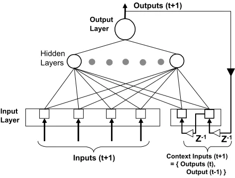
Based on the above propositions, a RNN architecture as shown in Fig. 3 has been developed to model the He´non map. It has been arrived at by experimentation

Fig. 2. Bifurcation Diagram of Heńon map (a two-dimensional dynamical system); (1)–(1), (2)–(2) and (3)–(3) are the cross-sections that show the first return maps or Poincare´ sections of the Heńon map in three different regions.

(5)

and is not sensitive to minor changes in the number of nodes in hidden layers etc. This model has four input nodes including the two delayed recurrence inputs as shown in the ﬁgure called context inputs and one output node. There are two hidden layers with 8 and 4 nodes respectively. It is trained using the standard Backpropa-gation algorithm. Solid lines in the ﬁgure indicate the training phase of the network and the dotted lines show the BD construction phase from the trained model. The model thus developed is tested for predicting the values in iterative mode away from the starting conditions.

2.2. Modelling He´non map through its observed data with a RNN

Heńon map is a discrete chaotic system that can be expressed in terms of mathematical equations. Most of the authors have observed Heńon map at one particular set of control parameters, where it shows chaotic nature; but have not modelled the whole system. In present work, the Heńon map is studied with all its control parameters to simulate the relevant objectives. The map is described by the following two iterative system equations:

Xnþ1¼1aX2nþbYn ð1Þ

Ynþ1¼Xn ð2Þ

whereXn+1andYn+1are the values of the He´non map at

(n+ 1)th time step,XnandYnare atnth time step andÔaÕ andÔbÕare constants. The values ofÔaÕranges from 0 to 1.4 andÔbÕ is taken as 0.3 for this study, but the provi-sion for varying this value is created.

To model the He´non map for creating its Bifurcation Diagram through RNN, ﬁrst a time-series data is gener-ated by using Eqs.(1) and (2). During the generationÔbÕ is kept constant at 0.3 andÔaÕis varied from 0 to 1.4 with increments of 0.01 (including both the values). The ini-tial conditions of the equations, X0 and Y0 are taken

as 0. For each value ofÔaÕ Eqs. (1) and (2)are iterated 22 times, thereby a total of 3102 patterns are generated. With this generated data, the proposed RNN model of the He´non map is developed.

As mentioned earlier the training of the RNN of the proposed architecture was carried out using the Back-propagation Algorithm which is commonly used [29]. The training was stopped when a low MSE level of 0.000001 was achieved and also further reduction did not happen. Using the network thus trained data was generated for drawing the Bifurcation Diagram of the system. Whereas it was observed that the BD generated was not sensitive to the changes in the architecture of the network but it was extremely sensitive to the MSE of the network.Fig. 4 shows a BD generated by this method (solid line) compared with the actual BD of the He´non map. It can be seen that the shape of the BD and the

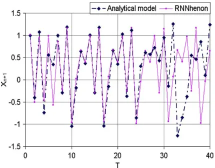
value of the Bifurcation point as generated by the RNN are very close to the real one. Further, the output series generated from the developed RNN model and the mathematical equations for the same initial condi-tions both, are compared inFig. 5. It can be seen from this ﬁgure that it is nearly in synchronism with the real one till 25 steps, showing the capability of the model. It compares favourably with the reported ﬁgures in [30]. It should be appreciated that longer predictions (through standard computer methods and analytical models) remain impractical due to extreme sensitivity of chaotic systems to initial conditions.

It can thus be seen that the predictive capabilities of the RNN needed for constructing a correct BD can be obtained by this approach but only at very low values of MSE of the network. This has been further studied in subsequent sections.

Fig. 4. Comparison of the Bifurcation Diagram of He´non map generated through the recursive analytical equation with the model generated diagram where the RNN is trained to MSE of 0.000001. Initial conditions in each case areb= 0.3,Xn= 0,Yn= 0 andavarying

from 0 to 1.4.

(6)

2.3. Training the RNN models with short multivariate observed series of data

The proposition that a RNN model can be used for modelling real-world systems requires that its trainabil-ity be tested with noisy data from short series. Under these conditions, its ability to recover the Lyapunov Exponents, which are measure of chaos in the system and are calculated by observing the divergence of nearby trajectories with time, and the accuracy of the generated Bifurcation Diagrams, may be regarded as tests for the capability of the procedure proposed.

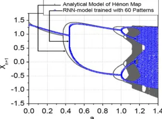
To validate this idea, a RNN model for the Heńon map has been trained with gradually increasing numbers of data points (obtained from the analytical model). Ef-fort has been made in each case to achieve a fixed MSE level of 0.000001.Fig. 6shows the attained values of the principal Lyapunov exponents with respect to the num-ber of training data patterns. It has been found that for example RNN of 4:8:4:1 architecture (the role of archi-tecture is further discussed in Section 3) trained with only 60 data points could emulate values close to real ones. The data series generated from this RNN yields the values of the first two exponents as 0.3950550 and

1.48133 comparing favourably with known values

of 0.4180959 and 1.6220686 respectively when a is 1.4 andbis 0.3. It is also seen fromFig. 7that the Bifur-cation Diagram generated from this series is very close to the one generated from longer data series obtained from the mathematical model.

It may also be observed that since only one step recurrence RNN model has been used, any two consec-utive data from relevant input–output pair are enough to form an input to RNN model and a continuous mul-tivariate time-series is not needed. This may be helpful in modelling real-world systems, where continuous obser-vations are diﬃcult.

2.4. Estimating the eﬀect of noise on the RNN models of the systems

The possibility of training a chaotic RNN model with a short data series or data sets having been demon-strated, it becomes important to study the effect of noise on the input parameters, observed time-series of the data and initial starting conditions of the systems, when these networks are to be used for predicting future val-ues away from a starting point. This has been studied by constructing the Bifurcation Diagrams of the Heńon map with different type of noise and is shown inFig. 8. The BD shown in Fig. 8(a) was generated through the recursive equations of the system where a noise of zero mean and uniform distribution was added to the b parameter of the Heńon map.Fig. 8(b) shows the same BD when it was generated using a RNN trained on the data used forFig. 8(a). It can be seen that the addition of noise causes scatter in the BD. This is in agreement with earlier observations reported in [31]. However, when this noisy data is used to train a RNN and the BD is plotted from the recursive outputs of this RNN, the BD is more like original one shown in Fig. 4 and the effect of noise is largely absent. This implies that the RNN architecture tends to reject the uncorre-lated information in the patterns during the learning phase itself.

Simulations have been further carried out to under-stand the effect of the noise on the control inputs as well as on the outputs of the chaotic systems through Heńon map. For these cases thus, the noise has been added to both theÔbÕparameter (equivalent of an input parameter to a system) of the Heńon map and as well as to the out-puts of the recursive analytical model. The BD con-structed through this data is shown in Fig. 8(c). Fig. 8(d) shows the same BD when it is generated using a RNN trained on the data used for Fig. 8(c). It is seen that with this type of noise the BD gets even more dis-persed but the RNN model is able to recover the shape once again. However, with this kind of noise the RNN

0 50 100 150 200

-1.2 -1.0 -0.8 -0.6 -0.4 -0.2 0.0 0.2 0.4 0.6

Laypunov Exponent

No. of Training Patterns Actual Value

Fig. 6. Evolution of Largest Lyapunov Exponent of He´non map at a= 1.4 andb= 0.3, calculated using the RNN models trained with diﬀerent number of patterns.

(7)

could not be trained to value of MSE below 0.00018. Despite this fact the RNN model could be used to con-struct the BD with the shape and the behaviour close to the actual BD.

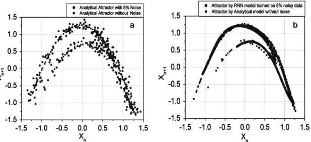
Further, a separate simulation has also been per-formed to examine the capability of RNN models in recovering the attractor of the system in the presence of large Gaussian noise. The role of attractor is impor-tant in chaotic processes as their time evolution is com-pletely governed by it, once the starting conditions are ﬁxed. For this purpose the simulation is carried-out on the time-series data of He´non map by adding 8% (equiv-alent of noise-to-signal ratio of 0.08) Guassian noise

with zero mean. An attempt has been made to construct the attractor directly from this time-series and also from RNN generated data, where the RNN was trained on the same noisy data. Fig. 9shows that the RNN based eﬀort is able to recover the attractor and this is compa-rable to eﬀorts reported in[30]using this method.

From the above observations, it can be seen that the RNN model based Bifurcation Diagrams created with the proposed approach, may have noise robustness at fairly high levels of noise (typically 3% or more) and these can be trained to fairly low values of MSE, in spite of the noise. This shows the suitability of this approach for handling real-world data from processes.

Fig. 8. Effect of noise on different parameters of the Heńon map in generating the Bifurcation Diagrams: (a) BD generated through the analytical model by inducing noise inÔbÕparameter of Heńon map, (b). The BD generated through a RNN model trained on the data used in (a), (c). BD generated through analytical model by inducing noise both inÔbÕparameter and the output of the of Heńon map i.e.Xn+1, (d). The Bifurcation

Diagram generated through RNN model trained on the data used in (b).

(8)

To test the susceptibility of initial starting conditions to random noise yet another simulation has been carried out where a Gaussian noise (3% equivalent of 0.03 noise-to-signal ratio) with zero mean has been added to all the input parameters at each time epoch and a per-manent change has also been made only in one of the input parameters. This change has the magnitude of three times the standard deviation of Gaussian noise. It can be seen from Fig. 10 that the bifurcation point gets shifted by the same magnitude as it would have without the noise.

3. Role of MSE of the network in the bifurcation patterns

The role of MSE could be very diﬀerent in a RNN trained to mimic a particular chaotic system compared to a standard RNN. In general for a feed-forward NN or a RNN the value of MSE represents the generalisa-tion capability of the model. A network with a low val-ues MSE is usually poor in prediction [32] on unseen data, but good on the trained data as compared to a net-work with coarse values of MSE, as with the reduction

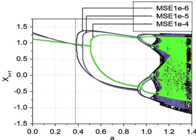
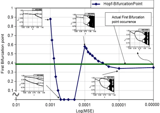
of the MSE the network starts to memorise. Thus, there is an optimum value of MSE for training. In contrast to this when a RNN represents a chaotic system evolving in time, a very low MSE alone can possibly make it memorise and represent a particular chaotic system. This property has been studied here through simulation. For this purpose the prediction capabilities of the devel-oped RNN models of Heńon map with different archi-tectures and trained to different MSE levels have been tested. It has been found that the architecture of the model has little effect on the Bifurcation Diagram once the architecture is not simpler than that of empirically suggested levels (Section 2.1). A set of Bifurcation Dia-grams generated with different MSE levels has been plotted inFig. 11. The ability of the models to generate a BD close to the actual BD has been observed with the MSE levels between 0.0001 and 0.000001.Fig. 12shows the patterns of improvement that occur in the prediction of the bifurcation point from the RNN model with the reduction in the MSE during the network training. At MSE level of 0.00003, the Heńon map generated through the RNN is close to the map generated by the analytical model.

It can be seen from Fig. 12that the RNN itself is a dynamical system and undergoes changes of behaviour as it is being trained. The MSE of the trained network influences the model Bifurcation point and other fea-tures significantly. However, at low MSE levels typically around 0.00001 it settles down to value close to the ac-tual values. One such convergence can be seen inFig. 12. However, it can be noticed that the overall shapes of Bifurcation Diagrams (thus the shape of attractors) do not change with MSE of training and they appear very early with coarse MSE levels even when Bifurcation point values etc. are still changing. Thus, the nature of the chaos in a chaotic system can be learnt easily with-out the need for hard training of the RNN. This phe-nomenon of early appearance of attractor appears to be similar to that identified by [33] as self emergence of chaos.

Fig. 10. The BD of a He´non map generated through a RNN model with Gaussian (rN= 0.03) noise added at each time epoch compared with the BD where a permanent change is done in the one of the control parameters takes place, in addition to the Gaussian noise. The zoomed box shows a clear shift in the bifurcation point occurs in spite of the noise.

(9)

However, real-world chaotic systems when observed through data always have a noise component in obser-vations and the RNNsÕ capability of modelling this should be ascertained. For this purpose two diﬀerent RNN models were trained by adding Gaussian noise in one case to only the input parameters, and in the sec-ond case to both the input and output parameters. It can be seen fromFig. 13that the correct value of Bifurcation point can be recovered in both the cases for up to 3% noise used for testing.

Further, a comparison of MSE levels needed is made, with a report from Jones et al. [16],where during the sychronisation eﬀorts of two low dimension chaotic neu-ral networks based maps, developed from analytical

models, it is shown that the MSE levels of the order of 0.000024 were needed for the models. The results ob-tained here during training of RNN models also show that the MSE reduction of RNN models to similar levels is necessary before the RNN models can mimic chaotic systems.

4. Control of discrete chaotic processes through their Recurrent Neural Network models

A major hurdle in controlling chaotic processes which have been observed only through their input and output data arises due to diﬃculty of building suitable models

Fig. 12. Changes in the Bifurcation point value (Hopf-Bifurcation) with the Mean Square Error in the training of the He´non map RNN model. With the decrease in the MSE, the RNN produces values closer to actual values.

0.1 0.2 0.3 0.4 0.5 0.6 0.7 0.8 0.9

0.000001 0.00001

0.0001 0.001

0.01

Log(MSE)

First Bifurcation point

1% nosie 2% noise 3% nosie

0.1 0.2 0.3 0.4 0.5 0.6 0.7 0.8 0.9

0.000001 0.00001

0.0001 0.001

0.01

Log(MSE)

First Bifurcation point

1% noise 2% noise 3% noise

a

b

(10)

from data. It has been shown in the previous sections that it can be overcome as a suitable models could be built through RNNs when trained to low MSE levels. It has also been shown that these RNN models could in-clude all the necessary input and output parameters of the system and could be MIMO models and thus could providing a scope for parameter based control. These RNN models may further have the capability of reject-ing observational and random noise in the observed data.

Besides the delayed feedback and the noise injection based techniques[13,34]for stabilising chaotic systems, the general approach of control of chaos relies on either changing the Bifurcation Point of the system to stable regions or stabilising the chaos at an unstable periodic orbit through what are called chaos controltechniques. Both these techniques merit evaluation for process con-trol. Also techniques which make it possible and even desirable to operate the process in chaotic conditions, but in more desirable regions, need to be studied.

In addition, it can be seen that the control of real-world processes rather than mathematical chaotic sys-tems, requires further constraints to be considered like:

(a) Real-time implementation of any proposed

method should be possible. Therefore, the compu-tational requirements when process is being run should be light.

(b) Number of intermediate steps needed to achieve the goal from the starting point should be a small to able to beneﬁt from the change.

(c) Output variations in the system should remain within some acceptable ranges when the control is being attempted.

Based on the above observations the following ways of controlling real-world chaotic process by exploiting the developed RNN models have been examined:

(1) Control of a chaotic process through its Bifurca-tion Diagram by moving the process to more acceptable conditions by changing the bifurcation points of the system through changes in the any of the of input parameters of MIMO–RNN model. (2) Control of chaotic systems in chaotic region

through changing over to more desirable attrac-tors of the system by changing input control parameters.

(3) Control of chaotic system with time varying small input impulses leading to small changes in initial conditions for stabilisation of the chaotic orbits on a unstable ﬁxed point of the system by an approach, using GA and RNN combination. This may be implemented under conditions where small changes in basic input conditions to the process may also take place.

4.1. Bifurcation control of a chaotic system

Once the BD has been constructed for a chaotic sys-tem from its observed data, the conditions where behavioural changes occur in the system become visible. Any change in the inputs (initial conditions) result in a new Bifurcation Diagram. This process of achieving control is referred to as Bifurcation Control (BC) in the literature. The bifurcation control is possible with changes in either a single parameter or multiple parameters.

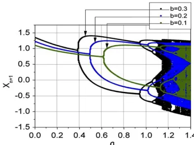
The RNN trained model of Heńon map has the equivalents of the input and output parameters of a process. Thus, the input parameters of this map either singly or in combination can be varied and their effect can directly be observed on the outputs of the chaotic process and the bifurcation phenomenon. This approach is suitable for changing the bifurcation point or alter-ing boundaries between chaotic, periodic and point attractor regions of the system as shown in Fig. 14for the Heńon map using RNN model. Here a and b are like input parameters where with the variation in the bifurcation point as observed on a parameter can be changed by changing the value of b. This approach is robust against process noise as has been demonstrated in Section 2.4 and shown in Fig. 10. Thus, it shows the possibility that if a RNN process model of the kind mentioned above has been built, it can be used to postpone the onset of chaos or for keeping the system in chaotic condition if so desired using the process variables.

The limitation of this method may be on the avail-ability of a suitable process parameter whose values can be changed signiﬁcantly without making the process throughputs or other features unacceptable.

This approach is light in terms of real-time computa-tional requirements and the desired shift can be obtained in few steps.

(11)

4.2. Controlling a chaotic process by driving the system towards a nearby desirable attractor

The OGY method and its variants rely essentially on perturbations (both in +ve and ve directions) to be given to the input conditions of the system to change the system evolution without permanently changing the initial (starting) condition, to stabilise the system on an unstable ﬁxed point. Thus the shape of the attrac-tor during the process does not change. However, in process control application it may be quite practical to switch to a nearby more desirable attractor in the phase space to achieve the objective of keeping the process moving towards stable zone of operation. This becomes a realisable alternative, as it may be possible to search and change the attractor in few steps using the RNN process model.

Most real-world processes as observed in [24] often have rich array of Bifurcation Diagrams and attractors. However, the He´non map which has been selected as a model for processes has a relatively simple attractor. Fig. 15(a) shows the starting attractor and Fig. 15(b) shows another attractor selected through the RNN model of the process. It can be seen that both are similar in shape, but since it occupies a smaller area, the process variations over this will be smaller. This limitation does not stop from using this attractor to stabilise the process on an unstable ﬁxed point on this attractor, using the procedure mentioned in the next section.

It can also be seen that, the switch to a new attractor cannot be made in one step, as the Recurrent Neural Network model has two part inputs consisting of the output in immediate past and the new condition being specified. Hence, although the new inputs will finally define the new attractor, it will be reached iteratively.

This approach requires searches to be made oﬀ-line through the model without disturbing the running pro-cess, making it a desirable method. Further, since the operation of the process can be brought to more accept-able levels of variation in a few steps makes it easy to implement. However, this can be realised only when

the process is having a variety of attractors and consid-erable changes in initial conditions are acceptable.

4.3. Stabilising a chaotic system where input conditions may change, through a step-by-step GA based search procedure

As observed earlier, the most successful method of controlling chaos has been through stabilisation of unstable periodic orbits using observations on the Poin-care´ section of the chaotic system through what is known as OGY method. This method works well when there is little or no noise [10,35] in the system. In this method it is necessary to wait before applying the con-trol action till system on its own reaches the vicinity of the unstable ﬁxed point. Sometimes it may take large number of cycles to reach the vicinity.

In a variant of OGY method proposed by Weeks and Burgees[12]to stabilise a process, the need for waiting is eliminated by training a Neural Network model to cal-culate the small impulses, to be given to control param-eters, such that it minimises the difference between the present and the next state of the plant, which makes the system drift towards a fixed point. In this approach the initial conditions (inputs) are to be kept constant while developing the Neural Networks, which is rather impractical for the process control application as input conditions may get unavoidably changed by a small amounts (above the noise level) and its effects need to be modelled. Further, in this approach for every attrac-tor (starting input conditions) a different Neural Con-troller has to be evolved which makes it a cumbersome proposition. Therefore, a procedure which takes these difficulties into account has been proposed, where for calculations of impulses to be given to the system, is based on an on-line search procedure with GA working on the full RNN model with all the process inputs. Thus, the initial conditions and other unavoidable changes can be taken into consideration while the on-line stabilisa-tion procedure is continuing. This procedure illustrated inFig. 16. The units on the left side of the figure act as a controller, consisting of the forward RNN model of the

(12)

R N N Model of Plant GA Plant (or) RNN Model of the Plant δp1 δp2 . . . δpn . . . p1 p2 . . . pn Z-1 X1 X2 . . . Xn 1 0 0 1 0 1 1 0 …..

Fitness of Individual Suggested Perturbations Previous State of the Plant State of the Plant

Updating the information on state of the plant

External Changes Inputs (initial conditions)

Control Parameters

→

Fig. 16. Block diagram of the GA-RNN based Chaos Controller for the stabilisation of a chaotic process.

Table 1

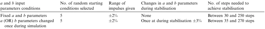
Simulation results for stabilisation of He´non map through GA-RNN searched impulses with and with-out small changes inaandbparameters during the process

aandbinput parameters conditions

No. of random starting conditions selected

Range of impulses given

Changes inaandbparameters during stabilisation

No. of steps needed to achieve stabilisation

Fixedaandbparameters 5 ±2% None Between 30 and 250 steps

a(OR)bparameters changed once during simulation

5 ±2% Once at during stabilisation ±3% Between 35 and 270 steps

-1.5 -1 -0.5 0 0.5 1 1.5

-1.5 -1 -0.5 0 0.5 1.5

X(n+1)

X( n+1 )

Starting point Stabilising onto Fixed point 1.35 1.36 1.37 1.38 1.39 1.4 1.41 1.42 1.43 1.44

0 40 80 120 160 200

Iterations a a-parameter 0.290 0.295 0.300 0.305 0.310

0 40 80 120 160 200

Iterations b b-parameter -1.5 -1 -0.5 0 0.5 1 1.5

0 40 80 120 160 200

Iterations X(n+1 ) X(n+1) X(n) Henon map uncontrolled a Controlled b c _d 1

Fig. 17. Stabilisation of chaos using RNN model and GA based searches through the input control parametersaandbof He´non map with only small variations from the present value. (a) Perturbations given toa. (b) Perturbation given tob. (c) Time–space evolution ofXn+1. (d) Phase–space

(13)

process coupled with a GA based search procedure. The right side ofFig. 16represents the process model, which in reality could be replaced with the real plant. Stabilisa-tion of the process can be started on the attractor visible from the initial starting conditions of the process.

To test the plausibility of the proposed GA + RNN approach, simulations were carried-out on the RNN model of the He´non map. Five random initial starting conditions were selected for stabilisation onto the unsta-ble ﬁxed point. First, the orbits were stabilised keeping the input conditions unchanged and then the simulation experiments were repeated by imposing one change in input conditions during stabilisation procedure.

Impulses given during the simulations were restricted to ±2%, a value above the real plant variations due to noise etc. which may be typically ±1% of the original parameter values and were applied to both a and b parameters of the He´non map. Using the GA based search criteria of minimising the diﬀerence between the present and the next state of the system it was found that between 30 and 250 steps were needed to stabilise the system on the initial attractor.

When a or b parameters were changed by ±3%

slightly above the impulse levels, once during the stabil-isation, between 35 and 270 steps were needed to achieve the same as shown inTable 1. Time steps evolution and phase-diagram etc. for a speciﬁc case are shown inFig. 17. From the above ﬁgure and table, it can be seen that the procedure works successfully even when the input conditions get altered and thus it suggests the possibility of using this procedure for real-world systems.

While the stabilisation of the He´non map onto a unstable ﬁxed point could be achieved in both the cases of either with or with-out small changes in input param-eters (a and b) during simulation but the need for the large number of steps to carry this out, and the real-time computation needed to achieve it may be a hindrance in the some real process control applications. Further, it can also be seen that the approach requires actual pro-cess to be continuously altered throughaandbimpulses which may not be practical. However, a plausibility of stabilising a real-world process with small changes in input conditions during stabilisation has been estab-lished, using the proposed approach.

5. Discussion and conclusions

One of the major problems in studying discrete pro-cesses plants for developing control models is that there is considerable noise in the observed parameters, and the plant operating conditions may not be easily changed to allow a particular study. It has been shown here that, since only data sets are to be fed to RNN models for training, and thus the control parameters may be chan-ged as often as required to run the real plant, without

regard to the modelling problems. This is so because the RNN models need only two consecutive operating data points (for one stage recurrence RNN models) to make one data set. This becomes an issue, if modelling has to be done through time-series method of analysis. Further, it has been shown that the noise sensitivity of RNN architecture to Gaussian noise is high enough and plant observational and parameter setting errors may not aﬀect the short term outcomes predicted by models, in spite of the essential long term unpredictabil-ity of chaotic systems.

The RNN models based approach proposed here, does not concentrate only on stabilising the chaotic orbit on a ﬁxed point or eliminating chaos by changing the bifurcation point etc., as the model remains relevant for running the process with the chaos as well. Running the system under the chaotic condition may even be desirable [1,13] and the control strategy followed have to be relevant to this. One approach based on changing the attractor of the chaotic process has been studied here.

The proposed strategies of controlling chaos in the process plants have been tested on a discrete chaotic system of Heńon map. The mathematical model of Heńon map has been widely studied in literature, which helps in assessing the performance of its RNN models. However, it should be noted that Heńon map has a chaos dimension of 2 and has only 2 control parameters, therefore while it may represent adequately some low dimension real-world chaotic systems, it cannot be used for generalisation of all chaotic process control prob-lems. Also, the results reported here remain true only for Heńon map (within the tested boundaries) and thus for other similar processes it may taken only as a plausibility.

The following conclusions have been drawn.

(1) Recurrent Neural Network based models for low dimensional real-worlds chaotic processes can be built from their short, and noisy observed data. These models can then be used for predicting the future evolution of the process state variables and constructing the Bifurcation Diagram of the systems.

(2) The role of RNN modelÕs MSE in modelling a pro-cess from its chaotic observed data is an important factor to be considered. Lesser the MSE the better are the predictions from the model for construct-ing Bifurcation Diagrams. When the value of MSE achieved is below a certain level a stable Bifurca-tion Diagram of the process can be created. (3) Through simulation results it is seen that the

(14)

(4) Through the MIMO–RNN models developed it is also shown that chaotic systems can be controlled through their attractors, by changing over to a nearby more desirable attractor of the process, using the visualisation and estimation capabilities of the model.

(5) Plausibility has been established for the control of a chaotic process whose input parameters change during operation, a situation close to reality, through stabilisation on an unstable ﬁxed point using the proposed RNN and GA based approach.

Acknowledgements

The authors are thankful to the ferroalloy producing organisation which has provided data for this study, and also SERC-DST, Government of India which provided grants as per Sanction no: SR/FTP/ET-83/2001 under its scheme of Fast track proposal for young scientists.

References

[1] E. Ott, C. Grebogi, J.A. Yorke, Controlling of chaos, Phys. Rev. Lett. 64 (1990) 1192–1196.

[2] W.L. Ditto, S.N. Rauseo, M.L. Spano, Experimental control of chaos, Phys. Rev. Lett. 65 (26) (1990) 3211–3214.

[3] M. van Duong, Method of controlling chaos in laser equations, Phys. Rev. E 47 (1) (1993) 714–717.

[4] G.L. Gray, Chaos in a class of satellite attitude maneuvers, Thesis, University of Wisconsin-Madison, Madison, 1993.

[5] A.P. Tsui, A.J. Jones, The control of higher dimension chaos: comparative results for the chaotic satellite attitude control problem, Physica D 135 (1–2) (2000) 41–62.

[6] A. Garﬁnkel, M.L. Spano, W.L. Ditto, J.N. Weiss, Controlling of cardiac chaos, Science 257 (1992) 1230.

[7] W.L. Ditto, L.M. Pecora, Mastering chaos: It is now possible to control some systems that behave chaotically. engineers can use chaos to stabilize lasers, electronic circuits and even the hearts of animals, Sci. Am. 269 (1993) 78–84.

[8] A.L. Fradkov, R.J. Evans, Control of chaos: Survey 1997–2000, in: Preprints of 15th IFAC World Congress on Automatic Control, Plenary papers, Survey papers, Milestones, Barcelona, 2002, pp. 143–154.

[9] R. Toral, Analytical and numerical studies of noise-induced synchronisation of chaotic systems, Chaos 11 (3) (2001) 665–673. [10] E.G. Chen, Controlling Chaos and Bifurcations in Engineering

Systems, CRS Press, Boca Raton, USA, 1999.

[11] X.D. Guanrong Chen, in: From Chaos to Order: Methodologies, Perspectives and Applications Series A, vol. 24, World Scientiﬁc, 1998.

[12] E.R. Weeks, J.M. Burgess, Evolving artiﬁcial neural networks to control chaotic systems, Phys. Rev. E 56 (2) (1997) 1531–1540. [13] K. Pyragas, Continuous control of chaos by self-controlling

feedback, Phys. Lett. A (1992) 421–428.

[14] A.J. Jones, A. Tsui, A.G. Oliveira, Neural models of arbitrary chaotic systems: construction and the role of time delayed feedback in control and synchronization, Complexity Interna-tional 9 (2002).

[15] G. Charles, M.D. Bernardo, M. Lowenberg, D. Stoten, X. Wang, Online bifurcation tailoring: an application to a nonlinear aircraft model, in: Proceedings IFAC 2002, IFAC, 2002.

[16] A.G. de Oliveira, A.P. Tsui, A.J. Jones, Using a neural network to calculate the sensitivity vectors in synchronisation of chaotic maps, in: Proceedings of the 1997 International Symposium on Nonlinear Theory and its Applications (NOLTAÕ97), vol. 1, Research Society of Nonlinear Theory and its Applications, IEICE, Honolulu, USA, 1997, pp. 46–49.

[17] J.S. Lee, K.S. Chang, Applications of chaos and fractals in process systems engineering, J. Process Control 6 (2/3) (1996) 71–87.

[18] A.P. Tsui, Smooth data modelling and stimulus-response via stabilisation of neural chaos, Ph.D. thesis, Department of Com-puting, Imperial College of Science, Technology and Medicine, University of London, 1999.

[19] B. Sivakumar et al., Dynamics of monthly rainfall-runoﬀ process at the gota basin: A search for chaos, Hydrol. Earth Syst. Sci. 4 (3) (2000) 407–417.

[20] F. Takens, Detecting strange attractors in turbulence: appeared in dynamical systems and turbulence, Lecture Notes in Maths, vol. 898, Springer-Verlag, Berlin, 1981, pp. 366–381.

[21] Po-Feng, J.-Z. Chu, S.-S. Jang, S.-S. Shieh, Developing a robust model predictive control architecture through regional knowledge analysis of artiﬁcial neural networks, J. Process Control 13 (2002) 423–435.

[22] V. Prasad, B.W. Bequette, Nonlinear system identiﬁcation and model reduction using artiﬁcial neural networks, Comput. Chem. Eng. 27 (2003) 1741–1754.

[23] J.-M. Kuo, J.C. Principe, B. de Vries, Prediction of chaotic time-series using recurrent neural networks, in: IEEE Workshop Neural Networks for Signal Processing, 1992, pp. 436–443. [24] J. Krishnaiah, C.S. Kumar, M.A. Faruqi, Constructing

bifurca-tion diagram for a chaotic time-series data through a recurrent neural network model, in: ICONIPÕ02 Proceedings, 2002. [25] A.L. Coryn, D. Bailer-Jones, J.C. MacKay, A recurrent neural

network for modelling dynamical systems, Comput. Neural Syst. 9 (1998) 531–547.

[26] Coherence resonance and excitability of optical systems, non-linear optics and laser physics. Available from:<http://www.phy. hw.ac.uk/resrev/ndos/cr.html>.

[27] R.C. Hilborn, Chaos and Nonlinear Dynamics: An Introduction for Scientists and Engineers, second ed., Oxford University Press, New York, 2000.

[28] A. Ro¨bel, The dynamic pattern selection algorithm: eﬀective training and controlled generalization of backpropagation neural networks, Tech. Rep., March 94.

[29] S. Haykin, Neural Networks: A Comprehensive Foundation, 2nd ed., Prentice-Hall, Englewood Cliﬀs, NJ, 1999.

[30] J.C. Sprott, Chaos and Time-Series Analysis, Oxford University Press, New York, 2003.

[31] K.R. Schenk-Hoppe´, Bifurcations of the randomly perturbed logistic map—numerical study and visualizations. Available from:

<http://www.iew.unizh.ch/home/klaus/logistic/intro.html>. [32] H. Jaeger, The Ôecho stateÕapproach to analysing and training

recurrent neural networks, Tech. Rep., 43, Forschungszentrum Informationstechnik, Sankt Augustin, Seiten, 2001.

[33] O. De Feo, Self-emergence of chaos in the identiﬁcation of irregular periodic behaviour, Chaos 13 (4) (2003) 1205– 1215.

[34] W. Freeman, H.-J. Chang, B. Burke, P. Rose, J. Badler, Taming chaos: stabilization of aperiodic attractors by noise, IEEE Trans. Circ. Syst. I: Fundam. Theory Appl. 22 (1997) 989–996. [35] F.C. Moon (Ed.), Dynamics and Chaos in Manufacturing