Candidate models for the IGRF-11th generation making use of
extrapolated observatory data
Aude Chambodut1, Benoit Langlais2, Michel Menvielle3,4, Erwan Th´ebault5, Arnaud Chulliat5, and Gauthier Hulot5
1Institut de Physique du Globe de Strasbourg (UMR 7516-CNRS, Universit´e de Strasbourg/EOST), Strasbourg, France 2Laboratoire de Plan´etologie et G´eodynamique de Nantes (UMR 6112-CNRS, Universit´e de Nantes), Nantes, France
3Universit´e Versailles-St Quentin; CNRS/INSU, LATMOS-IPSL, Paris, France 4D´epartement des Scinces de la Terre, Univ. Paris Sud, Orsay, France
5Institut de Physique du Globe de Paris, ´Equipe de G´eomagn´etisme (UMR 7154-CNRS, Universit´e Paris Diderot), Paris, France
(Received December 8, 2009; Revised June 20, 2010; Accepted June 22, 2010; Online published December 31, 2010)
Three candidate models are produced in response to the call for IGRF-11 models. A main field model around epoch 2005.0 is based on one year of Ørsted and CHAMP measurements, and is proposed for the definitive model for epoch 2005.0. A main field model around epoch 2009.5, based on two months of CHAMP measurements and extrapolated to 2010.0, is proposed as a main field model for epoch 2010.0. A secular variation model valid for 2010.0–2015.0, based on the extrapolation through exponential smoothing of observatory monthly mean values, is proposed as a predictive secular variation model. Comparison of similar extrapolations made for previous IGRF generations with actual observations are presented and discussed.
Key words:Magnetic field, main field, secular variation, modeling, IGRF, time extrapolation.
1.
Introduction
The International Geomagnetic Reference Field (IGRF) is a time series of Gauss coefficients, describing the large-scale part of the Earth’s magnetic field of internal origin. Since the 9th generation of IGRF (Macmillanet al., 2003) coefficients are given up to degree and order 13. IGRF mod-els therefore describe the Main Field (MF) and its Secu-lar Variation (SV), whose sources are located in the Earth’s outer core.
The 11th generation of the IGRF model is an update of the previous generation, with new definitive MF co-efficients for epoch 2005.0, provisional (and predictive) MF coefficients for epoch 2010.0 and predictive SV coef-ficients for epoch 2010–2015 (up to degree and order 8). In this paper, we present the candidate models that were pre-pared and submitted by a consortium made of the Institut de Physique du Globe de Strasbourg, the Laboratoire de G´eodynamique et de Plan´etologie de Nantes, the Laboratoire Atmosph`eres, Milieux, Observations Spatiales and the Institut de Physique du Globe de Paris. In the fol-lowing we describe the datasets and the methodology, with special attention to the predictive SV, by analyzing similar predictions that were made in the frame of the 8th genera-tion of the IGRF (Langlais and Mandea, 2000; Mandeaet al., 2000b).
2.
Main Field Model for Epoch 2005.0
The MF model at epoch 2005.0 is made of definitive coefficients and aims at describing the large-scale internal
Copyright cThe Society of Geomagnetism and Earth, Planetary and Space Sci-ences (SGEPSS); The Seismological Society of Japan; The Volcanological Society of Japan; The Geodetic Society of Japan; The Japanese Society for Planetary Sci-ences; TERRAPUB.
doi:10.5047/eps.2010.06.006
part of the magnetic field of the Earth as accurately as possible for a given epoch within the model limitations. We computed a parent model, using standard data selection criteria and model parameterization.
2.1 Data
Our model is based on CHAMP and Ørsted satellite mag-netic field measurements. These spacecrafts were launched in 1999 and 2000, respectively (Olsenet al., 2000; Reigber et al., 2002). These successful missions considerably im-proved the way the magnetic field is described and mod-eled. Prior to these spacecrafts, and with the exception of the MAGSAT mission, it was indeed difficult to accurately describe the main magnetic field, even in the frame of IGRF models (Loweset al., 2000).
The dataset spans a twelve-month period, from July 2004 to June 2005. It contains Ørsted and CHAMP, vector (north-wardBX, eastwardBYand downwardBZfield components) and total field measurements. Data (with 1s sampling rate) were first decimated along track, keeping only one mea-surement out of ten. Then a selection scheme was used to minimize the magnetic fields of external origin. First, only scalar measurements were considered above 50◦ absolute geomagnetic latitude. Second, a local time 22:00–06:00 se-lection was applied. Third, activity indices were used to select the quietest measurements.
K-derived geomagnetic indices, and in particular theKp
planetary index, are classically used to achieve this selec-tion. The success of this approach for estimating external source contamination in the magnetic data used for internal field calculations results from the fact that K indices de-rive from ground-based magnetic variations, thus providing reliable upper bounds to the mid-latitude, external transient fields at satellite altitude, as demonstrated by Mareschal and
746 A. CHAMBODUTet al.: CANDIDATE MODELS FOR IGRF-11
Menvielle (1986).
It is however well established that the intensity of geo-magnetic activity is statistically more intense during night-time than during day-night-time. One way to improve the se-lection of satellite measurements with respect to magnetic quietness is therefore to characterize geomagnetic activity at a regional scale, so that its LT dependence is taken into account. Menvielle and Paris (2001) proposed a longitude sector index, theaλindex, derived usingKindices from the amobservatory network. Theaλindex thus provide a better
selection of magnetic quietness time intervals, and it en-ables one to achieve a more accurate modelling, as shown for instance by Cohen and Achache (1990) and Thomson and Lesur (2007). The reader is referred to Menvielle and Berthelier (1992) or Menvielleet al.(2010) for further de-tails onKpandamindices.
Another way to improve the selection of satellite mea-surements with respect to magnetic quietness is to reduce the duration of the time window over which the geomag-netic index is computed. Menvielle (1979) showed that the K index is a proxy of the magnetic energy density re-lated to the geomagnetic activity, because the time scale of the observed geomagnetic variations is less than the 3-hour length of the interval for whichK is measured. He however also showed that such a range index is no longer a proxy of this energy if the length of the interval over which it is measured is significantly smaller than 3 hours. Reducing the length of the time interval over which the index is cal-culated implies the use of another proxy. Because of the Poynting theorem, the root mean square (rms) value of the irregular variations in the horizontal field components is di-rectly related to the magnetic energy related to the geomag-netic activity. Indeed, empirical histograms of the range vs rms distributions atamobservatories and for 3-hour
in-tervals show that their range is statistically proportional to the rms value, with a 30–50% dispersion (Menvielleet al., 2010). In fact, Menvielle (2003) already proposed to derive new geomagnetic indices based on the rms of the irregular variations in the horizontal components: theαmnn indices
(unit: nT), where nn is the length (in minutes) of the consid-ered time interval. In the present study, we use such rms in-dices with a 30-minute resolution interval, theαm30 indices.
They are derived from minute values recorded at a network of about 20 INTERMAGNET mid-latitudes observatories evenly distributed in longitude in both hemispheres.
In the following, only measurements associated with
αm30 ranging between 0 and 4 nT were kept. An additional
selection was done with respect to theDstgeomagnetic
ac-tivity index, with a limit set to|Dst(t)|<30 nT and a
max-imum time derivative of|d Dst(t)/dt| <10 nT/hr. We
fur-ther decimated the dataset, by keeping a maximum of one measurement in each 1◦×1◦bin for each month. Whenever more that one measurement was present, the one associated with lowest indices was kept. The final dataset contains 144004 (CHAMP scalar), 88971 (CHAMP vector triplets), 92790 (Ørsted scalar), and 13674 (Ørsted vector triplets) measurements. The distribution of the final dataset was checked: there is at least one measurement in each 3◦×3◦ bin.
2.2 Modeling and results
We used the above described dataset to derive a magnetic field model for epoch 2005.0. It is computed up to degree and order 15 for the main field, with a SV up to degree and order 8. The external field is modeled up to degree and order 2, with a degree-1Dstdependency.
Ørsted data were weighted using an anisotropic scheme, to reflect the uncertainty related to attitude provided by the Star Imager (Holme, 2000). In contrast, as the selected CHAMP data were all acquired when both CHAMP star imagers were operating, all CHAMP data were isotropically weighted. Ørsted and CHAMP data were assigned a relative 1/σ2 weight, withσ equal to 2 nT and 3 nT for CHAMP and Ørsted, respectively. For each satellite dataset, equal weights were given to scalar and vector measurements. A further sin(θ)weighting scheme was applied to counterbal-ance the denser data distribution near the poles.
The inverse problem was linearized and solved using a least square method (Cain et al., 1967). The choice of the model for the first iteration has no importance on the final result (Ultr´e-Gu´erard, 1996). We did not use any regularization. Convergence was reached after 3 iterations. The final rms differences for the twelve-month model are:
Ørsted: 4.14 nT (scalar)
Ørsted: 3.41 nT (BB), 11.43 nT (B⊥), 6.77 nT (B3).
CHAMP: 7.87 nT (scalar)
CHAMP: 4.87 nT (BX), 4.86 nT (BY), 5.22 nT (BZ)
As expected, Ørsted rms differences are larger in the di-rection that is perpendicular to the field and the Star Imager bore sight (B⊥), and lower in the direction of the field (BB) and in the third complementary direction (B3). CHAMP
rms differences are larger than those of Ørsted, but this is likely related to the lower altitude of the spacecraft, which orbited closer to unmodeled ionospheric sources. Although those rms differences could have led us to modify our data weighting scheme, we decided not to do so, for simplicity. Our candidate model for IGRF-11 epoch 2005.0 is the trun-cated (to degree and order 13) and rounded (to the nearest 0.01 nT) version of the model based on our twelve-month dataset.
3.
Main Field Model for Epoch 2010.0
The IGRF-11 describes the magnetic field of internal ori-gin up to degree and order 13 at epoch 2010.0. We com-puted this predictive model in two steps. First, we devel-oped an internal field model based on very recent CHAMP satellite magnetic measurements. Second we extrapolated this model to epoch 2010.0 using by-products of the SV model series as described in Section 4.
3.1 Data
In order to minimize the errors related to model extrap-olation, we chose to build our model using the most recent available magnetic measurements. We used CHAMP scalar and vector data between June and July 2009, which was the last period when both vector and scalar data were available when this model was produced.
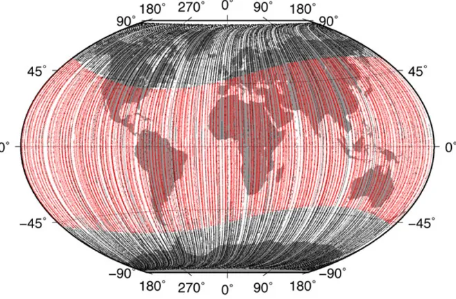
Fig. 1. CHAMP data distribution used in the elaboration of the main-field model for epoch 2010.0:redpoints correspond to vector triplets data and
blackpoints to scalar measurements.
5 nT and a maximum time derivative of |d Dst(t)/dt| <
3 nT/hr; and for the planetary index: Kp(t) < 1+ and
Kp(t ±3 hr) < 2−. The magnetic sectorial index αm30
we used for the 2005.0 model was not considered here, as it was not yet available.
The data distribution was finally homogenized as much as possible, keeping a maximum of 10 measurements per 3◦ ×3◦ bin. When a bin contained more than 10 mea-surements, the furthest ones from 00:00 local time were withdrawn. The global geographical distribution of data was checked: there are at least two measurements in each 4◦×4◦bin over the entire surface (Fig. 1). The final dataset consists of 66027 scalar measurements and 55111 vector triplets. This large number of measurements (for a two-month period, and when compared to the twelve-two-month pe-riod of the previous section) may be explained by the fact that June/July 2009 was a very quiet magnetic period at the end of a solar minimum.
3.2 Modeling and results
The dataset described is used to derive a main field model up to degree and order 15, without any secular variation, but with an external field up to degree and order 2. Because we set a much narrow range for the Dstselection than for the
2005.0 model, no Dst dependency was introduced. Equal
weights were given to scalar and vector measurements. A sin(θ) weighting scheme was used to counterbalance the denser data distribution near the poles.
We used the same inversion method as in Section 2.2. The final rms differences are 10.18 nT for scalar data, and 6.60, 4.05 and 11.90 nT for theBX,BYandBZcomponents, respectively.
The model we computed has a mean date equal to 2009.485. We extrapolated this model to 2010.0. We used two annual SV models (each one valid for one year and cen-tered on the first day of the year, as described in Section 4): SV2009 (multiplied by 0.015, i.e. the time difference be-tween the model date and 2009.5) and SV2010 (multiplied
by 0.5, i.e. the time difference between 2009.5 and the fi-nal model date 2010.0). Only terms for degree lower or equal to 8 were extrapolated, terms for higher degrees were unchanged. The 2010.0 model may therefore contain some error associated with (1) the extrapolation for degreen ≤ 8 and (2) the non extrapolation of higher degree terms. Our candidate model for IGRF-11 epoch 2010.0 is the trun-cated (to degree and order 13) and rounded (to the nearest 0.01 nT) version of this extrapolated parent model.
4.
Internal Field Secular Variation for Epoch
2010.0 to 2015.0
The last model that is proposed for the IGRF-11 is the secular variation one. This model aims at describing the time evolution of the magnetic field between 2010.0 and 2015.0, assuming a constant rate of change. It is therefore a predictive model, based on the extrapolation of past vari-ations. One method (as used by other groups, e.g. Th´ebault et al., 2010, this issue) is to jointly model the magnetic field and its secular variation, using temporal splines or lin-ear/quadratic variation. An alternative choice is to model only magnetic time variations as observed in magnetic ob-servatories. This is the approach we chose here, because it allows the temporal variations of the magnetic field to be better identified and separated from the geographical vari-ations, thanks to the observatory database. It also mini-mizes possible contamination by the primary ionospheric field since observatories are located below the ionosphere. 4.1 Data
Our approach is similar to that of Langlais and Mandea (2000) which they used to propose a candidate SV model for IGRF-08. However, whereas Langlais and Mandea (2000) computed SV models by first difference of succes-sive MF models, we directly computed annual SV models from the difference of observatory annual means, bypassing in fact the intermediate computation of MF.
748 A. CHAMBODUTet al.: CANDIDATE MODELS FOR IGRF-11
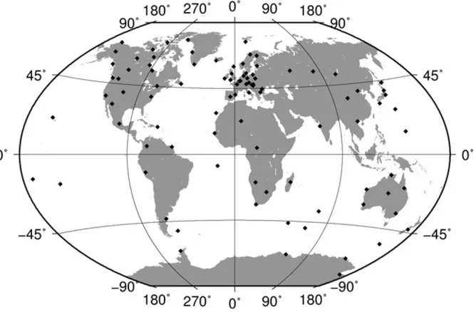
Fig. 2. The 96 geomagnetic observatories used to calculate the secular variation model series.
World Data Center C1 in Edinburgh, and monthly mean values were computed. We disregarded observatories for which time series were shorter than 11 years. Out of a gross total of 200 observatories providing hourly mean val-ues between 1980 and 2008, only 96 observatories were se-lected for this study. Many of them were rejected because they ceased operations before (or did not provide data after) 2007, some others were rejected because of very long data gaps. Time series were plotted and individually checked to disregard possible outliers, which were removed.
The obtained monthly mean values were compared with two other datasets: the IPGP monthly means database (Chulliat and Telali, 2007), and the values computed (un-til 1998) by Langlais and Mandea (2000). This dual com-parison allowed some spurious jumps to be identified and eliminated. The final dataset consists of 96 observatories (list available on request; see the geographical distribution on Fig. 2), providing monthly mean values at least between 1997 and 2007 or 2008 (inclusive). In some cases, missing values were linearly interpolated, the longest gap being 24 months.
These 96×3 time series were extrapolated until the end of 2015, using an exponential smoothing scheme, which is described as (Gardner, 2006):
St =αXt−It−p
+(1−α) (St−1+Tt−1)
Tt =γ (St−St−1)+(1−γ )Tt−1
It =δ (Xt−St)+(1−δ)Tt−p
ˆ
Xt =St+mTt+It−p+m
At a given timet, the smoothed signalSdepends on the observed signal X, on the estimated seasonal component I (of period p), as well as on the estimated additive trend T. The relative importance of these terms is determined by the smoothing parametersα, γ andδ, which describe the relative importance of the previous observation, of the ex-ponential trend and of the seasonal part, respectively. The period of the seasonal signal was set to twelve months.
These parameters were automatically adjusted, by mini-mizing the rms difference between true observations and smoothed ones. The best fit was automatically computed for each time series and component, using the Statistica software ( cStatsoft). Series are then extrapolated in time using the previously derived smoothing parameters, to ob-tainXˆduringmtime increments. In the vast majority of the cases,δwas found to be equal to 0, i.e. the seasonal part was kept constant throughout the whole time series. Most of the time,γ was also found to be small, close to 0.05, meaning that the previously observed trend was only slowly varying. The last smoothing parameterαhad larger values, between 0.5 and 1.
Time series of true, interpolated and extrapolated data were plotted and individually examined. In some cases where the result of the extrapolation appeared odd, extrapo-lations were compared with provisional hourly means (ob-tained from observatories or from INTERMAGNET), to validate extrapolated trends. All of them were visually in-spected, confirming the relevance of the smoothing and ex-trapolation scheme for recent changes. Annual means were thereafter derived from the monthly means, between 1980.5 and 2015.5. We then computed annual differences at each observatories, from 1981.0 to 2015.0.
Predicting the time variations of the magnetic field is challenging. The accuracy of our extrapolations cannot be tested for now, but we can test the level of confidence of the method by comparing past predictions to actual observa-tions. Langlais and Mandea (2000) used a similar scheme when they extrapolated observatory monthly mean values over intervals of two to three years until the end of 2000. They considered 93 observatories in their study. Because some of them were closed, and the data at some others were degraded, we were able to compare their predictions to ac-tual monthly mean values at only 54 observatories.
be-20800 20900 21000
1990 1992 1994 1996 1998 2000 2002
0 20 40 60
1990 1992 1994 1996 1998 2000 2002
0 20 40 60 42300
42400 42500 42600
1990 1992 1994 1996 1998 2000 2002
0 20 40 60
32600 32700 32800
1990 1992 1994 1996 1998 2000 2002
0 20 40 60
1990 1992 1994 1996 1998 2000 2002
0 20 40 60 32300
32400 32500 32600 32700 32800
1990 1992 1994 1996 1998 2000 2002
0 20 40 60
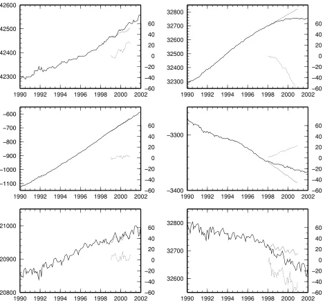
Fig. 3. Comparison of observed (solid black line) and predicted (solid gray line) monthly mean values for Chambon La Forˆet (CLF) and Kanoya (KNY) observatories by Langlais and Mandea (2000). Differences (dashed gray line) are shown on the right axis.
tween 3.82 and 22.33 nT for BX, 1.77 and 17.58 nT for BY, and 3.59 and 35.39 forBZ. The average rms difference is 8.8, 6.1 and 11.45 nT for the three components, respec-tively. Only 2 or 3 resulting annual means were extrapo-lated, and it is not possible to derive robust statistics for these.
We show on Fig. 3 two examples of such extrapolations, made by Langlais and Mandea (2000). The first one is in Chambon La Forˆet (CLF-France), and represents well other observatories in Europe, where predictions matched observations relatively well. The second one is in Kanoya (KNY-Japan), and is one of the observatories where the predictions failed. There is a clear change in the trend of all three components around 1998, which is not reproduced by the extrapolation. At the end of the 3-year extrapolation interval, errors on field components reached up to 60 nT.
The abrupt change observed around 1998 at KNY may be related to a geomagnetic jerk, occurring at or near epoch 2000 (Mandeaet al., 2000a; Mauset al., 2005). At CLF,
this jerk occurred in 1998.0, i.e. prior to the extrapolation period. An abrupt change also happened at KNY around the same period, but this occurred during the extrapolation pe-riod. Clearly, abrupt changes in the secular variation trend can not be predicted by our method. On the other hand, the physics associated with magnetic jerks is still poorly un-derstood, and it is not possible to accurately predict these events (Jackson and Finlay, 2007).
4.2 Modeling
750 A. CHAMBODUTet al.: CANDIDATE MODELS FOR IGRF-11
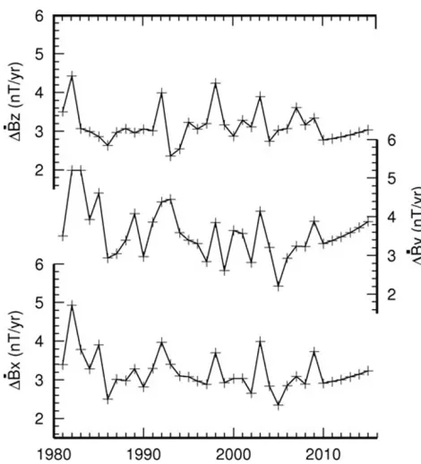
Fig. 4. Temporal evolution of the rms differences associated with the annual SV models. Models posterior to 2009 are based on extrapolated data.
The same modeling scheme as previously was used. Each individual observatory annual mean (based on real observa-tions or on extrapolated ones) was weighted accordingly to the inverse of the mean distance to the four closest observa-tories in the four NW, NE, SE and SW quadrants, as detailed in Langlais and Mandea (2000). The fit to theBX˙ , BY˙ and
˙
BZfield component differences varies from one year to the next one (Fig. 4). Prior to 2008.0 (i.e., for models based on true observations), rms errors ranged between 2.50 and 4.92 nT.yr−1forBX˙ , 2.21 and 5.20 nT.yr−1forBY˙ , and 2.35 and 4.43 nT.yr−1for BZ˙ . After 2008 (i.e. for models based on extrapolated data), errors on field component variations ranged between 2.89 and 3.72 nT.yr−1forBX˙ , 3.23 and 3.88 nT.yr−1for BY˙ , and 2.77 and 3.34 nT.yr−1forBZ˙ .
Interestingly, there is an apparent correlation between the rms errors for each field component differences. Rms max-ima are observed in 1992–1993, 1998, and 2003. These actually correspond to periods when jerks were observed (Chambodut and Mandea, 2005; Chulliat et al., 2010). There is a last occurrence over 2007–2009. It might be ar-tificial in our study, because the computed rms differences are based on a mix of observed and extrapolated annual dif-ferences, but a jerk was nonetheless observed in 2007 and 2008 at some observatories, mostly at mid-latitude (Chulliat et al., 2010).
4.3 Results
Our series of models is made of 35 SV models, from 1981.0 to 2015.0. This long time series allowed us to check the validity of the modeled secular variation prior to epoch 2008. We averaged the last six models, with a weight of 1/2 for SV2010 and SV2015, and 1 for the others. Our final candidate model is therefore centered on 2012.5. Individual coefficient errors associated with the averaging process (i.e.
based on the rms differences between the final candidate model and the six models above mentioned) are very small and meaningless, and do not represent the possible time evolution of the SV. We chose instead to compute the rms differences between SV2005, SV2006, SV2007 and SV2008 models on one hand, and their arithmetical mean on the other hand. These individual coefficient rms are actually proportional to the observed changes of the SV (i.e. the secular acceleration) during these four years.
Our SV candidate model for IGRF-11 (valid for the pe-riod 2010.0–2015.0 and centered in 2012.5) is a rounded (to the nearest 0.01 nT/yr) version of this model, up to de-gree/order 8, with associated rms errors.
5.
Discussion and Conclusion
We presented three candidate models for IGRF-11. These models were computed using very simple parametrization, without regularization or temporal splines. Our model for epoch 2005.0 is based on one year of satellite measurements, and the parent model has a trun-cated linear secular variation up to degree and order 8. The parent model of our candidate model for epoch 2010.0 is based on only two months of CHAMP measurements, then extrapolated with a predictive SV. Our predictive secular variation model for epoch 2010.0–2015.0 is built with observatory annual differences based on the extrapolation of observatory monthly means.
The comparison of past predictions to actual observations sets the limits of our approach. As expected, time extrapo-lation of monthly (or annual) mean series is valid provided that these variations remain more or less linear. Differences between our extrapolated annual means and the observed ones at a given observatory may be larger than 100 nT at the end of the considered 2010–2015 period. These relatively large errors have to be compared to the differences between the IGRF-8 and IGRF-9 at epoch 1995.0 or at epoch 2000.0 (definitive coefficients for these epochs were adopted for IGRF-9), which reached 200 to 300 nT in many locations at the surface of the Earth (Chambodutet al., 2005).
During the past decade, the successful Ørsted and CHAMP satellite missions have allowed major break-throughs in the description and understanding of the mag-netic field of the Earth (Hulotet al., 2007). The upcom-ing SWARM mission will include two spacecrafts flyupcom-ing side-by-side at a low altitude, and a third one at a higher orbit (Friis-Christensen et al., 2006). This configuration will help to better characterize the small scales of the mag-netic field, which include the time evolution of the field. However, this mission will be fruitful only if the efforts in promoting and maintaining surface magnetic observatories are pursued. The recent or scheduled closure of such mag-netic observatories is worrying, because the success of the SWARM mission partly relies on the long term observation of the current magnetic field.
con-tributed to the development, the launch and the ground section of the Ørsted and CHAMP missions. The CHAMP data were kindly provided by V. Lesur and M. Hamoudi (GFZ). The Ørsted data were collected by IPGP M. Roharik (IPGP). All maps have been plotted using the General Mapping Tool Software (Wessel and Smith, 1991). This study was partly supported by CNES. This is IPGP contribution N◦3036.
References
Cain, J. C., S. J. Hendricks, R. A. Langel, and W. V. Hudson, A proposed model for the International Geomagnetic Reference Field -1965,J. Ge-omag. Geoelectr.,19, 335–355, 1967.
Chambodut, A. and M. Mandea, Evidence for geomagnetic jerks in com-prehensive models,Earth Planets Space,57, 139–149, 2005. Chambodut, A., B. Langlais, and M. Mandea, Candidate main-field models
for the Definitive Geomagnetic Reference Field 1995.0 and 2000.0,
Earth Planets Space,57, 1197–1202, 2005.
Chulliat, A. and K. Telali, World monthly means database project, inProc. of the XIIth IAGA Workshop on Geomagnetic Observatory Instruments, Data Acquisition and Processing. Publs. Inst. Geophys. Pol. Acad. Sc., C-99, 268–274, 2007.
Chulliat, A., E. Th´ebault, and G. Hulot, Core field acceleration pulse as a common cause of the 2003 and 2007 geomagnetic jerks,Geophys. Res. Lett.,37, L07301, doi:10.1029/2009GL042019, 2010.
Cohen, Y. and J. Achache, New global vector magnetic anomaly maps derived from MAGSAT data,J. Geophys. Res.,95, 10783–10800, 1990. Friis-Christensen, E., H. L¨uhr, and G. Hulot, Swarm: A constellation to study the Earth’s magnetic field,Earth Planets Space,58, 351–358, 2006.
Gardner Jr., E. S., Exponential smoothing: The state of the art—Part II,Int. J. Forecasting,22, 637–666, 2006.
Holme, R., Modeling of attitude error in vector magnetic data: application to Østed data,Earth Planets Space,52, 1187–1197, 2000.
Hulot, G., N. Olsen, and T. J. Sabaka, The present field, inTreatise on Geophysics, vol. 5, Geomagnetism vol. 5, edited by M. Kono, 33–75, Elsevier, Amsterdam, The Netherlands, 2007.
Jackson, A. and C. Finlay, Geomagnetic secular variation and its applica-tions, inTreatise on Geophysics, vol. 5, Geomagnetism vol. 5, edited by M. Kono, 147–193, Elsevier, Amsterdam, The Netherlands, 2007. Langlais, B. and M. Mandea, An IGRF candidate main geomagnetic field
model for epoch 2000 and a secular variation model for 2000–2005,
Earth Planets Space,52, 1137–1148, 2000.
Lowes, F. J., T. Bondar, V. P. Golovkov, B. Langlais, S. MacMillan, and M. Mandea, Evaluation of the candidate Main Field model for IGRF 2000 derived from preliminary Østed data,Earth Planets Space,52, 1183– 1186, 2000.
Macmillan, S., S. Maus, T. Bondar, A. Chambodut, V. Golovkov, R. Holme, B. Langlais, V. Lesur, F. Lowes, H. L¨uhr, W. Mai, M. Man-dea, N. Olsen, M. Rother, T. Sabaka, A. Thomson, and I. Wardinski, The 9th-Generation International Geomagnetic Reference Field,Phys. Earth Planet. Inter.,140, 253–254, 2003.
Mandea, M. and B. Langlais, Observatory crustal magnetic biases dur-ing MAGSAT and Østed satellite missions,Geophys. Res. Lett.,29, doi:10.1029/2001GL013693, 2002.
Mandea, M., ´E. Bellanger, and J. L. Le Mou¨el, A geomagnetic jerk for the end of the 20th century?,Earth Planet. Sci. Lett.,183, 369–373, 2000a. Mandea, M., S. Macmillan, T. Bondar, V. Golovkov, B. Langlais, F. Lowes, N. Olsen, J. Quinn, and T. Sabaka, International geomagnetic reference field—2000,Pure Appl. Geophys.,157, 1797–1802, 2000b.
Mareschal, M. and M. Menvielle, On the use ofKindices to define max-imum external contributions to MAGSAT data at mid-latitudes,Phys. Earth Planet. Inter.,43, 799–204, 1986.
Maus, S., S. McLean, D. Dater, H. L¨uhr, M. Rother, W. Mai, and S. Choi, NGDC/GFZ candidate models for the 10th generation International Ge-omagnetic Reference Field,Earth Planets Space,57, 1151–1156, 2005. Menvielle, M., A possible geophysical meaning of K indices,Ann.
Geo-phys.,35, 189–196, 1979.
Menvielle, M., On the possibility to monitor the planetary activity with a time resolution better than 3 hours, inProceedings of the Xth IAGA Workshop on Geomagnetic Instruments, Data Acquisition and Process-ing, edited by L. Loubser, 246–250, HMO publication, 2003. Menvielle, M. and A. Berthelier, TheK-derived planetary indices:
descrip-tion and availability,Rev. Geophys. Space Phys.,29, 415–432, 1991 (er-ratum,30, 91, 1992).
Menvielle, M. and J. Paris, Theaλlongitude sector geomagnetic indices,
Contrib. Geophys. Geodes.,31, 315–322, 2001.
Menvielle, M., T. Iyemori, A. Marchaudon, and M. Nose, Geomagnetic indices, inIAGA Sopron Special Book Series, edited by M. Mandea and M. Korte, 2010.
Olsen, N., R. Holme, G. Hulot, T. J. Sabaka, T. Neubert, L. Toffner-Clausen, F. Primdahl, J. Jorgensen, J. M. Leger, D. Barraclough, J. Bloxham, J. Cain, C. Constable, V. Golovkov, A. Jackson, P. Kotze, B. Langlais, S. Macmillan, M. Mandea, J. Merayo, L. Newitt, M. Purucker, T. Risbo, M. Stampe, A. Thomson, and C. Voorhies, Ørsted initial field model,Geophys. Res. Lett.,27, 3607–3610, 2000.
Reigber, C., H. L¨uhr, and P. Schwintzer, CHAMP mission status,Adv. Space Res.,30, doi:10.1016/S0273-1177(02)00276-4, 2002.
Th´ebault, E., A. Chulliat, S. Maus, G. Hulot, B. Langlais, A. Chambodut, and M. Menvielle, IGRF candidate models at times of rapid changes in core field acceleration,Earth Planets Space,62, this issue, 753–763, 2010.
Thomson, A. W. P. and V. Lesur, An improved geomagnetic data selection algorithm for global geomagnetic field modelling,Geophys. J. Int.,169, doi:10.1111/j.1365-246X.2007.03354.x, 2007.
Ultr´e-Gu´erard, P., Du pal´eomagn´etisme au g´eomagn´etisme spatial: anal-yse de quelques s´equences temporelles du champ magn´etique terrestre, PhD thesis, Institut de Physique du Globe de Paris, 1996.
Wessel, P. and W. H. F. Smith, Free software helps map and display data,
EOS Trans. AGU,72, 441, 1991.