Source model of the 2005 Miyagi Oki, Japan, earthquake estimated from broadband strong motions

Source model of the 2005 Miyagi-Oki, Japan, earthquake estimated from

broadband strong motions

Wataru Suzuki and Tomotaka Iwata

Disaster Prevention Research Institute, Kyoto University, Gokasho, Uji, Kyoto 611-0011, Japan

(Received April 1, 2007; Revised September 30, 2007; Accepted October 23, 2007; Online published November 30, 2007)

We estimate the source model of the 2005 Miyagi-Oki earthquake, which consists of two source patches called “strong motion generation areas (SMGAs)”, to explain the broadband strong motions. The location of the first SMGA is determined from the arrival time differences between the first motion and the first pulse in theP-wave portion. Based on the broadband waveform modeling obtained using the empirical Green’s function method, we estimate the parameters of the two SMGAs. The estimated location of the two SMGAs coincides with the two major large slip areas inferred from the inversion of strong-motion and teleseismic waveforms, which implies that the broadband strong motion of the 2005 Miyagi-Oki earthquake mainly radiates from the asperities. The deeper SMGA has a larger stress drop (34.1 MPa) than the shallower one (17.6 MPa). Comparison of the locations of SMGAs between the 2005 and 1978 Miyagi-Oki earthquakes suggests that they do not overlap with each other. The interplate earthquakes, including this event, were found to have smaller SMGAs than those predicted from the relationship of crustal earthquakes for a given seismic moment. This implies that the stress drop of the SMGAs for interplate earthquakes is larger than that for crustal earthquakes.

Key words:2005 Miyagi-Oki earthquake, empirical Green’s function method, broadband strong motion, source model, interplate earthquake.

1.

Introduction

The study of kinematic waveform inversion of strong-motion records has revealed a detailed source process and allowed a better understanding of seismic sources. In most cases, these source images represent the source pro-cess of low-frequency wave radiation or low-frequency source model because the theoretical Green’s function for strong-motion records is less reliable and because wave-form matching is difficult for the frequency ranges higher than 1 Hz. In order to learn about the source physics and the asset it represents in terms of strong-motion prediction, recent studies have attempted to construct source models re-lated to broadband wave radiation (e.g., Zenget al., 1993; Nakaharaet al., 2002; Shiba and Irikura, 2005). One of the more successful approaches is the empirical Green’s func-tion (EGF) simulafunc-tion with a simple source patch model characterized within the total rupture area (e.g., Kamae and Irikura, 1998; Miyake et al., 2003; Morikawa and Sasa-tani, 2004). The EGF method is a technique used to synthe-size seismic records by summing up the observed records of small earthquakes. It can therefore simulate realistic wave-forms up to high frequencies that are affected by minute heterogeneous propagation-path structures. The assumed source model consists of a (multiple) rectangular area(s) that has no explicit heterogeneity of slip, rise time, and rup-ture velocity inside of it. Miyakeet al. (2003) named this area “strong motion generation area (SMGA).” The SMGA

Copyright cThe Society of Geomagnetism and Earth, Planetary and Space Sci-ences (SGEPSS); The Seismological Society of Japan; The Volcanological Society of Japan; The Geodetic Society of Japan; The Japanese Society for Planetary Sci-ences; TERRAPUB.

represents the large-slip velocity area extracted in the to-tal slip area to explain the characteristics of broadband (ap-proximately 0.1–10 Hz) strong motions.

Miyakeet al. (2003) showed that the SMGAs of crustal earthquakes that were estimated independently of low-frequency strong-motion waveform inversions correspond to the asperities inferred by those inversions with respect to the location and size. Moreover, they found that the total area of SMGAs is consistent with the empirical relationship between the total asperity area and the seismic moment de-rived by Somervilleet al. (1999). The SMGA stress drop is estimated to be approximately constant for crustal earth-quakes over the moment range between 1.83×1016 _and 1.38×1018 _{N m (M}

W4.8–6.0). This scaling relationship has been confirmed from more crustal earthquakes of either small or large magnitude (e.g., figure 7 of Suzuki and Iwata, 2006). Although some researchers have investigated the SMGAs of large subduction-zone interplate earthquakes, such as the 1994 Sanriku Haruka-Oki earthquake (Miyahara and Sasatani, 2004) and the 2003 Tokachi-Oki earthquake (Kamae and Kawabe, 2004), such studies are relatively few in comparison to the number carried out on crustal earthquakes. Suzuki and Iwata (2005) have estimated the SMGAs for moderate-sized interplate earthquakes that oc-curred at the subducting Pacific sea plate near Northeast Japan with a seismic moment ranging from 1.16×1018_to 3.36×1019_{N m (M}

W6.0–7.0). In order to understand the source characteristics of interplate earthquakes in relation to broadband strong motions, it is necessary to examine the scaling relationship of SMGAs by accumulating the results obtained from similar analytic procedures.

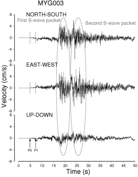
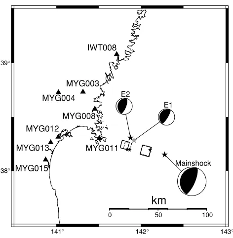
Fig. 1. Location of the 2005 Miyagi-Oki earthquake determined by the JMA. The focal mechanism is obtained from the prompt report of the Harvard CMT project. The velocity waveforms at the K-NET station, i.e., MYG003, is shown in Fig. 2.

On August 16, 2005, an earthquake with an MJMA = 7.2 (magnitude determined by the Japan Meteorological Agency, JMA) occurred offshore of Miyagi Prefecture (Miyagi-Oki region), Japan. The latitude, longitude, and depth of the JMA hypocenter are 38.150◦N, 142.278◦E, and 42.0 km, respectively. Figure 1 shows the epicenter and fo-cal mechanism of this earthquake. This 2005 Miyagi-Oki earthquake is thought to be an interplate earthquake that oc-curred between the subducting Pacific plate and the North American plate. The Miyagi-Oki region has repeatedly ex-perienced M7.5-class earthquakes at average intervals of 37 years, and there was a high probability that it would ex-perience the anticipated earthquake (The Headquarters for Earthquake Research Promotion, 2005). Hence, the ques-tion of whether the 2005 Miyagi-Oki event is the character-istic earthquake or not attracts interest. The last large event in this region occurred in 1978 with anMJMA=7.4. There-fore, the relationship between the 2005 and 1978 events has been examined. Based on the relocated aftershock distribu-tion and slip distribudistribu-tion obtained by teleseismic waveform inversion, Okadaet al. (2005) concluded that the 2005 event ruptured a part of the source area of the 1978 event. Yag-inumaet al. (2006) also concluded from several inversion results that one of the asperities of the 1978 event was rup-tured during the 2005 event. Wu and Koketsu (2006) dis-cussed the rupture pattern, comparing the source processes inverted from the strong-motion and teleseismic records for the 2005 event and strong motions for the 1978 event. Based on the broadband strong-motion simulation, Kamae (2006) reported that one source patch near the hypocenter is

Fig. 2. Velocity waveforms of station MYG003 obtained from a single integration of acceleration record without applying a filter. Two wave packets can be observed in theS-wave portion.

similar between the 2005 and 1978 earthquakes in terms of location and stress drop, whereas the landward one is dif-ferent.

In this paper, we estimate the source model of the 2005 Miyagi-Oki earthquake, which is composed of SMGAs, with the aim of gaining an understanding of the source process that generates broadband strong motions, and we assess its relationship to the 1978 event. We propose a methodology based on an objective procedure. We also examine the scaling relationship of SMGAs for the inter-plate earthquakes around Japan. We use the strong-motion records of K-NET and KiK-net maintained by the National Research Institute for Earth Science and Disaster Preven-tion (NIED).

2.

Features of the Observed Strong Motions

gen-Strike

Hyp0

Hyp1

dip Ray

Fig. 3. Schematic illustration of locating Hyp1 by following the procedure of Takenakaet al. (2006). Two-dimensional coordinate systemξ1–ξ2is

spanned along the strike and dip directions. Its origin is the hypocenter, Hyp0.is the angle between the ray and the vector to Hyp1 measured at Hyp0.

erates the first S-wave packet SMGA1 and that generating the second, SMGA2. In Fig. 2, there are two wave packets in the P-wave portion that correspond to the two S-wave packets mentioned above. A close look at theP-wave por-tion reveals that the amplitude of the waves immediately af-ter theP-wave arrival is considerably small and that the first wave packet arrived approximately 2.3 s after the first P-wave arrival. This indicates that SMGA1, where the first S-wave packet is generated, is different from the hypocenter. Based on the features of the observed waveforms described above, we can assume that the source model is composed of two SMGAs that are located away some distance from the hypocenter of the 2005 Miyagi-Oki earthquake.

It is necessary to know the time of the S-wave arrival in order to be able to estimate the location of the SMGAs by simulating whole S-wave records. However, the first S-wave motions of this earthquake are difficult to detect because it is veiled under the second P-wave packet and P-coda waves. We will, therefore, firstly determine the location of the rupture starting point of SMGA1 by using the difference in the arrival times of the firstP-wave motion (P0) and the first P-wave packet (P1). After locating the rupture starting point of SMGA1, the relative location of SMGA2 to SMGA1 and various parameters, such as size, stress drop, and the rise time of the SMGAs, are inferred by fitting the synthetic waveforms to the observed ones using the arrival time of the firstS-wave packets, which are assumed to be generated by SMGA1, as a reference time.

3.

Locating Rupture Starting Point of SMGA1

We estimate the location of the rupture starting point of SMGA1 (Hyp1), relative to the hypocenter determined by the JMA (Hyp0), by following the procedure of Takenaka et al.(2006), who investigated the 2005 West Off Fukuoka Prefecture earthquake. In the P-wave records of the 2005 West Off Fukuoka Prefecture earthquake, the small initial phase preceded the large main phase by a few seconds, similarly to the 2005 Miyagi-Oki earthquake. The differ-ence in the arrival times between the first motion (P0) from the hypocenter and the main phase (P1) generated from SMGA1,TP1−P0, can be modeled by Eq. (1).

TP1−P0=T0−lcos/VP (1)

Fig. 4. Distribution of the stations used to locate Hyp1, indicated by triangles. The location denoted by the star is the epicenter of the 2005 Miyagi-Oki earthquake determined by the JMA, or Hyp0. The rectangle shows the search range for Hyp1 location.

T0 is the delay time of the SMGA1 rupture relative to the origin time, is the angle between the departing ray and the vector toward Hyp1 measured at Hyp0,lis the distance between Hyp0 and Hyp1, andVP is theP-wave velocity of

the source region. If we use the two-dimensional coordinate system spanned on the fault plane, in which theξ1-axis is along the strike direction and theξ2-axis is along the down-dip direction, the distancelcan be expressed as Eq. (2).

l=

ξ2

1 +ξ22 (2) The geometrical setting of this problem is illustrated in Fig. 3. It is assumed here that the waves are radiated from Hyp0 and Hyp1 with the same take-off angles.

We determine the location of Hyp1 expressed by theξ1–

Table 1. Estimated Hyp1 location and rupture delay time with parameters used for the grid search. The parameters are relative to the source information obtained by the JMA. ξ1 andξ2 are along the strike and

dip directions, respectively. Average value and standard deviation of the location andT0 listed lower are estimated from the 2000 data sets of

TP1−P0randomly perturbed±0.2 seconds with probability of 50%.

ξ1(km) ξ2(km) T0(s)

Search range −15 to 15 −20 to 20 0 to 5

Grid size 0.5 0.5 0.1

Estimated value −1.0 16.5 4.3

Average value −1.14 16.22 4.28

Standard deviation 0.31 1.20 0.11

2.0 2.5 3.0 3.5 4.0

T

(s)

0.2 0.4 0.6 0.8 1.0 Observed Time Difference Estimated Relation

Fig. 5. Relationship between the observedTP1−P0and cos. The solid

line is the linear Eq. (1) for which the estimated parameters are substi-tuted.

CMT project. The take-off angles required for the calcula-tion of cos andVP (7.53 km/s) are assumed by referring

to the JMA table used for hypocenter determination. A set of parameters that gives the least residual value is listed together with the search range in Table 1. The search range is also shown on the map in Fig. 4. The location of Hyp1 is estimated to be approximately 16 km closer to the coastline than Hyp0. Figure 5 shows the observedTP1−P0 versus cos with Eq. (1) calculated from the determined parameters. The observed data follow the linear relation of Eq. (1).

To examine the effect of an error in phase detection, we prepare 2000 data sets that consist ofTP1−P0randomly perturbed from the observed data by+0.2 or−0.2 s with a 50% probability for each station. The same procedure is applied to these data sets to estimate the location of Hyp1. The estimated parameter set listed in Table 1 is that obtained the most often during these 2000 trials. The average values and standard deviations are listed in Table 1. The standard deviation of the locationξ2is larger than that ofξ1because

ξ2 has a trade-off with T0, which may be caused by poor station coverage along the dip-direction. Nevertheless, it can be said that an error of phase picking does not affect the estimated result to any great degree.

l

w

L

W

r

r

r

subfault (

i,j

)

EGF event

SMGA

Fig. 6. Schematic illustration of the EGF method using SMGA. The black star denotes the rupture starting point of SMGA. Each subfault of SMGA and the EGF event have the same size.

4.

Estimation of the Source Model from

Broad-band Waveform Simulation

4.1 Formulation of the EGF method

In the previous section, we determined the relative lo-cation and the relative time for the start of the rupture of SMGA1 to the hypocenter. Based on this result, we will es-timate the broadband source model or the parameters of the SMGA1 and SMGA2 by simulating strong motions over a wide frequency range using the EGF method proposed by Irikura (1986).

Irikura’s method is formulated on the basis of the self-similar scaling law of the source parameters and theω−2 source spectral model. From the self-similar scaling law of the source parameters between large and small earthquakes (Kanamori and Anderson, 1975), the seismic momentM0, fault lengthL, fault widthW, rise timeT, and the amount of the slipDare related, as shown in Eq. (3).

(M0/m0)1/3=L/l =W/w=T/t =D/d =N (3)

where capital and small letters denote large and small events, respectively. The constant N represents a ratio of these parameters between large and small earthquakes. Miyakeet al.(2003) used the term and concept of SMGA as the rupture area from the viewpoint of strong-motion simu-lation. Hereafter, we treatL,W,T, andDas the parameters of SMGA of a large earthquake or a target earthquake. We treatN as the integer number related with the division of SMGA into subfaults (Fig. 6).

accelera-U

/

u

2005 Miyagi-Oki / Aftershock (9061813)

IWT008

Fig. 7. Amplitude spectral ratio of the target event record to the EGF event one. (a) Schematic illustration of the spectral ratio of the two events. fcm

and fcaare the corner frequencies of the target and EGF events, respectively. (b) The observed spectral ratio of the 2005 Miyagi-Oki earthquake at

eight K-NET stations used for the EGF simulation. Picked flat levels,U0/u0andA0/a0are indicated with arrows.

tion spectra.

U0/u0=M0/m0=C N3 (4)

A0/a0=C N (5)

These two parameters, i.e.,C andN, are required for the EGF waveform synthesis.

The waveform record of the target eventU(t)is calcu-lated by summing up the record of a small or EGF event u(t)using Eqs. (6) and (7).

In these equations,VSisS-wave velocity around the source

region, and VR is the rupture velocity. ξi j is the distance

between the subfault (i,j) and the hypocenter of the main-shock, andr0,r are respectively the hypocentral distances of the target and the EGF events, andri jis the distance

be-tween the subfault (i,j)and the station (Fig. 6). We use NxandNwinstead ofNto distinctly express the number of

subfaults the SMGA has been divided into along the strike and dip directions, respectively. By convolving the func-tionF(t), we adjust the slip time function of the EGF event to that of the target event. In other words, we sum up the records of the EGF event on the slip. F(t)is expressed in the discretized form as Eq. (8), which is introduced by Irikuraet al.(1997). artificial periodicity outside of analyzing frequency band.

Nt is the number of summation of EGF in time on one

subfault.

4.2 Analytic procedure

It is necessary for the EGF simulation to determine C and N from the spectral ratio of the target event to the EGF event, as mentioned in the previous subsection. Equa-tions (4) and (5) are those for the case with single SMGA. Since the 2005 Miyagi-Oki event can be explained by two SMGAs from observed waveforms, we need to introduce the modified equations for determining C and N. If two SMGAs have the sameCandN values, which implies that they have the same stress drop and spatial dimension, then Eqs. (9) and (10), introduced by Yokoi and Irikura (1991) and Miyakeet al.(1999), are used instead of Eqs. (4) and (5):

U0/u0=2C N3 (9) A0/a0=

√

2C N. (10)

We consider not only the case of two SMGAs having the sameC value but also the cases when one SMGA has aC value 1.5 times or twice as large as the other.

We adopt the records of an MJMA = 4.1 aftershock, which occurred on September 6, 2005, as EGF. This after-shock is appropriate for the EGF event because it occurred within the rupture area expected from the waveform inver-sion and has a focal mechanism similar to that of the target event (Fig. 8). The focal depth determined by the JMA is 45.1 km and the seismic moment determined by F-net of NIED is 1.44×1015N m. The eight K-NET stations shown in Fig. 8 are used in this analysis. Figure 7(b) shows the S-wave spectral ratios calculated using a 30-s time window. By following Eqs. (9) and (10) and introducing differentC values for the two SMGAs, we obtain five combinations for CandNx,Nw,Nt, as shown in Table 2. For Combinations

3 and 5, we use a different N value betweenNx, Nwand

Ntin order to make the combination more flexible to obtain

Fig. 8. Distribution of the K-NET stations (solid triangle) and the epicen-ter of the mainshock and the EGF event used for waveform simulation, together with the estimated SMGAs projected on the slip distribution inferred by Wu and Koketsu (2006) by using strong-motion and tele-seismic data. Their slip distribution is shifted to match the epicenter de-termined by ERI to that dede-termined by the JMA. Red inverted triangles are KiK-net stations used for the comparison of waveforms with those obtained by Kamae (2006), which are shown in Fig. 14. Purple open squares are F-net stations used to examine the influence of the assumed seismic moment on the low-frequency component (Fig. 13).

We employ the genetic algorithm (GA) for estimating the source model in order to evaluate broadband waveforms by minimizing the following misfit function (Suzuki and Iwata, 2005, 2006).

misfit=

(uobs−usyn)2dt

u2_obsdt u2 syndt

+

(eobs−esyn)2dt

e2_obsdt e2 syndt

(11)

Here,uis the velocity waveform bandpass-filtered between 0.2 and 1 Hz, while eis the envelope of the acceleration waveform bandpass-filtered between 0.2 and 10 Hz. The lower frequency limit is determined from the S/N ratio of EGFs. The acceleration envelope is calculated from the root-mean-square (RMS) of acceleration records with a 1-s time window. The misfit is calculated over 20 s, beginning from 4 s before the arrival time of theS-wave from SMGA1 for two horizontal components, covering the whole rupture duration. The misfit function (11) is similar to that used in Miyakeet al.(1999, 2003), who utilized the displacement waveforms and acceleration envelopes. We use the mis-fit function for the velocity waveforms up to 1 Hz instead of displacement to see the source rupture model that con-trols broadband strong motions related to earthquake disas-ter (e.g., Kawase, 1998).

The model parameters estimated by the GA are the size and rise time of the EGF event, the rupture starting sub-fault of the two SMGAs, and the starting point and time of

Table 2. Combination of theCandN values of the two SMGAs. Nx,

Nw areN value for summation of EGF along the strike and the dip directions in Eq. (6), respectively, andNtis that for summation

regard-ing time in Eq. (8). The values of Combination 1 are calculated from Eqs. (9) and (10).

SMGA1 SMGA2

Combination C Nx Nw Nt C Nx Nw Nt

1 4.0 10 10 10 4.0 10 10 10

2 5.0 9 9 9 3.3 11 11 11

3 5.6 9 9 8 2.8 12 12 11

4 3.3 11 11 11 5.0 9 9 9

5 2.8 12 12 11 5.6 9 9 8

SMGA2 rupture. Since the number by which SMGAs are divided into subfaults, i.e., Nx and N_w, has already been

determined, the determination of the size of the EGF event or subfault corresponds to an estimation of the size of SM-GAs. The rise time within the SMGAs is also calculated from the multiplication of the rise time of the EGF event by Nt. The shape of the EGF event or subfault is assumed to be

square. Table 3 shows the search range and search interval of the model parameters. The rupture starting subfault of each SMGA is found amongNxsubfaults in the shallowest

row aligned along the strike direction. The rupture inside the SMGAs is assumed to propagate radially from Hyp1 or Hyp2. The rupture velocity (VR) inside SMGAs is fixed

in each GA search. We assume four different rupture ve-locities: 2.7, 3.15, 3.6, and 4.05 km/s, which correspond to 60%, 70%, 80%, and 90% of theS-wave velocity (4.5 km/s) of the source region, respectively. Since there are the five combinations ofCandN, as listed in Table 2, and the four rupture velocities, a total of 20 cases are taken into account. The GA code is based on the package PIKAIA (Charbon-neau, 1995). The numbers of the populations (individuals) and generations (iterations) for the GA search are 200 and 200, respectively. Since the GA is the heuristic search, we attempt ten searches with different initial populations or pa-rameter sets to confirm the robustness.

4.3 Result

Among the 20 cases tested, Combination 5 shown in Ta-ble 2 withVR =3.15 km/s gives the smallest misfit value.

TheCvalue of SMGA2 in this combination is twice as large as that of SMGA1, which implies that the stress drop of SMGA2 is twice that of SMGA1. The estimated model pa-rameters of the GA search are listed in Table 3. Three of the ten GA trials for Combination 5 withVR =3.15 km/s

give this estimated parameters, and one trial returns almost the same parameters. The obtained result is satisfactorily robust, although some trials could not reach the global min-imum. For this case, we perform the GA search using the misfit of the displacement waveforms instead of the velocity ones and obtain the same result as that shown in Table 3. Ta-ble 4 shows the SMGA parameters of this model. The seis-mic moment of each SMGA is calculated by multiplying the moment of the EGF event byC×Nx×Nw×Nt. The stress

Table 3. Search range, interval, and estimated value of model parameters of the GA search.landτare the fault length and the rise time of the EGF event, respectively. The rupture starting subfault of each SMGA is expressed by using the coordinates in the SMGA, as shown in Fig. 6, spanned along the strike and dip directions.ξ1, ξ2are the locations of Hyp2 from the Hyp0 along the strike and dip directions, respectively.T0is the rupture

time relative to the rupture of SMGA1.

EGF event Rupture starting subfault Rupture of SMGA2

l(km) τ(s) SMGA1 SMGA2 ξ1(km) ξ2(km) T0(s)

Search range 0.1 to 5.0 0.01 to 0.3 Among shallowest row −30 to 30 10 to 50 3.0 to 13.0

Search interval 0.1 0.01 Every subfault 0.5 0.5 0.1

Estimated value 0.8 0.03 (4, 1) (9, 1) 4.5 38.0 7.0

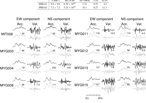
Table 4. Estimated parameters of two SMGAs from the EGF simulation.S,M0,σ,τ, andT0denote the area size, seismic moment, stress drop, rise

time, and rupture starting time, respectively.T0is measured from the origin time determined by the JMA.

S(km2_{) M}

0(N m) σ(MPa) τ(s) T0(s)

SMGA1 9.6×9.6 6.39×1018 17.6 0.33 4.3 SMGA2 7.2×7.2 5.23×1018 34.1 0.27 11.3

EW component

NS component

Acc.

Vel.

Acc.

Vel.

IWT008

MYG003

MYG004

MYG008

MYG011

MYG012

MYG013

MYG015

0 s 20 s

EW component

NS component

Acc.

Vel.

Acc.

Vel.

Fig. 9. The fittings of the acceleration envelopes (0.2–10 Hz) and velocity waveforms (0.2–1 Hz) used as a target for the genetic algorithm. The upper black traces are observed, and the lower gray traces are simulated. The maximum values of the observed data are indicated between the observation and the simulation. The units for acceleration envelopes and velocity waveforms are cm/s2and cm/s, respectively.

joint inversion of the strong-motion and teleseismic data. These researchers used the hypocenter determined by the Earthquake Research Institute (ERI), University of Tokyo, which is different from that used in this study. Therefore, the slip distribution shown here has been shifted from that based on ERI to that determined by the JMA in order to match the epicenters. Wu and Koketsu (2006) assumed a slightly different fault plane (strike 211◦and dip 23◦) from that which we assume; in accordance with the CMT solu-tion they determined the fault plane from the teleseismic body wave inversion. In Fig. 8, two SMGAs with Hyp1 and Hyp2, which are denoted by squares with stars, respectively, correspond to the two large slip regions or asperities. Hyp2 is located approximately 38 km away from the hypocenter

and approximately 22 km away from Hyp1.

The rupture delay time of SMGA2, relative to that of SMGA1, is estimated to be 7.0 s independently of locating Hyp2. The apparent rupture velocity between Hyp1 and Hyp2, calculated from the distance divided by the delay time, is 3.17 km/s. This is almost the same as the estimated rupture velocity inside the SMGAs.

EW component

NS component

Acc.

Vel.

Disp.

Acc.

Vel.

Disp.

IWT008

MYG003

MYG004

MYG008

MYG011

MYG012

MYG013

MYG015

0 s 20 s

Fig. 10. The fittings of the broadband waveforms (0.2–10 Hz) in acceleration, velocity, and displacement. The upper black traces are observed, and the lower gray traces are simulated. The maximum values of the observed waveforms are indicated between the observation and the simulation. The units for acceleration, velocity, and displacement waveforms are cm/s2_{, cm/s, and cm, respectively.}

to 10 Hz. Although some discrepancy can be seen, the EGF simulation satisfactorily reproduces the main characteristics of the observed waveforms for all stations. These good fits are achieved from acceleration to displacement, which im-plies that the broadband strong motions are simulated well. The clear second pulse waves observed at northern stations, such as IWT008, MYG003, and MYG008, are well

0 50 100

Fig. 11. Comparison of the SMGAs obtained in Section 4 using the EGF event, E1, and those obtained by using the different EGF event, E2. Rectangles with solid lines are SMGAs using E2, and rectangles with broken lines are those with E1. The epicenters and focal mechanisms of the mainshock, E1, E2 are also shown.

5.

Examination of the Obtained Source Model

There may be a possibility that the source model obtained in Section 4 is under some adverse influence of the condi-tions in the analysis, such as the selection of EGF event, the picked flat levels in Fig. 7(b), and the site response of the used stations. In this section, we will confirm the reliability and applicability of the obtained SMGA model.

5.1 Influence of the selection of the EGF event

We examine the influence of the selection of EGF event on the result from the analysis using the different EGF event. The EGF event used in Section 4 (called E1 in this subsection) is one of the most appropriate candidates for the EGF event from the viewpoint of the magnitude, location, and focal mechanism. We find that anMJMA = 4.1 earth-quake that occurred near the hypocenter of E1 on Novem-ber 8, 2004, before the mainshock, can be considered to be the other EGF candidate, called E2 hereafter (Fig. 11). The records of E2 are obtained at all the eight stations used in Section 4. Using the records of E2 as EGF, we estimate the source model by the same analytic procedure as that de-scribed in Section 4. Since the spectral ratios of the main-shock to E2 closely resemble those to E1, we assume the same combinations ofC andN values determined for the analysis with E1.

Figure 11 shows the estimated location of the two SM-GAs together with those obtained from the analysis with E1. We define the term SMGA1(E1) as SMGA1 determined by the analysis with E1, and SMGA2(E1), SMGA1(E2), SMGA2(E2) in a similar way. We can see that SMGA1(E2) is located at almost the same place as SMGA1(E1), and that SMGA2(E2) overlaps with SMGA2(E1). Table 5 shows the parameters of the SMGAs. VR inside the SMGAs is

Table 5. Estimated parameters of two SMGAs from the analysis with the different EGF.S,M0,σ,τ, andT0represent the same parameters as

estimated to be 3.6 km/s. Although the stress drop of SMGA2(E2) is smaller than that of SMGA2(E1), the pa-rameters estimated here are similar to those obtained in Sec-tion 4, especially for SMGA1. The tendency that the stress drop of SMGA2 is larger than that of SMGA1 is the same. A comparison of the observed and synthetic waveforms is shown in Fig. 12. The frequency ranges of these waveforms are 0.2–10 Hz except for the displacement waveforms of some stations where the EGF records have insufficient S/N ratio for the low-frequency range. The simulated wave-forms fit to the observed ones well. Although the estima-tion for SMGA2 is slightly different in terms of locaestima-tion and stress drop, the result obtained in Section 4 is confirmed to be satisfactorily robust to the difference in the selection of the EGF event. Since the GA search for the analysis with E1 is more stable and the EGF records seem to have better S/N ratio than those for the analysis with E2, we will treat the model estimated in Section 4 as the obtained source model and base on discussions on it.

5.2 Applicability of the estimated SMGA model for the lower frequency range

Spectral ratios in Fig. 7(b) show the fall-off in the low-frequency range because the records of EGF have a low S/N ratio for these frequency range. The picked U0/u0 in Fig. 7(b), which is 8000, is actually smaller than the seismic moment ratio of the mainshock to the EGF event, which is approximately 37,000 calculated from the moment tensor solutions by F-net. The obtained source model is constructed with approximately one fifth of the total seismic moment based on the waveform simulation between 0.2 and 10 Hz.

EW component

NS component

Acc.

Vel.

Disp.

Acc.

Vel.

Disp.

IWT008

MYG003

MYG004

MYG008

MYG011

MYG012

MYG013

MYG015

0 s 20 s

0.41

0.77 1.74

0.92 0.69

Fig. 12. Comparison of the observed and the synthetic waveforms obtained by using the records of E2 as EGF for frequency range between 0.2 and 10 Hz. The frequency range of the displacement waveforms at IWT008 is 0.25–10 Hz and those at MYG003 and MYG011 are 0.33–10 Hz since the S/N ratio of the EGF records at these stations is not enough for 0.2 Hz. The upper black traces are observed, and the lower gray traces are simulated. The maximum values of the observed waveforms are indicated between the observation and the simulation. The units for acceleration, velocity, and displacement waveforms are cm/s2, cm/s, and cm, respectively.

waveforms since the lower frequency content dominates in the observation. Nevertheless, we can see some similarity for displacement waveforms filtered between 0.1 and 10 Hz. Figure 13(b) shows the comparisons between the observa-tion and simulaobserva-tion of the displacement amplitude spectra

1e-05 0.0001

0.001 0.01

0.1 1 10 100

0.01 0.1 1 10

EW component

0.01 0.1 1 10

NS component

KSN

1e-05 0.0001

0.001 0.01

0.1 1 10 100

Displacement Spectra (cm*s)

0.01 0.1 1 10

Frequency (Hz)

0.01 0.1 1 10

TYS

(b)

Not Filtered

EW component

NS component

Acc.

Vel.

Disp.

Acc.

Vel.

Disp.

KSN

27 3.1 2.41 29 2.7 2.62

TYS

34 1.5 1.46 25 1.1 1.78

KSN

24 3.0 0.94 25 2.3 0.86

TYS

30 1.4 0.72 21 1.1 0.27

0 s 20 s 40 s

0.1-10.0Hz

(a)

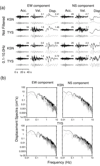
Fig. 13. Comparison of the observation and the simulation assumed by the obtained source model at the F-net stations. The location of the two stations is shown in Fig. 8. (a) Comparison of waveforms in terms of acceleration, velocity, and displacement for two frequency bands: full-frequency (upper panel) and 0.1–10 Hz (lower panel). The upper black traces are observed, and the lower gray traces are simulated. The maximum values of the observed waveforms are indicated above the observation. The units for acceleration, velocity, and displacement waveforms are cm/s2_{, cm/s, and cm,}

respectively. (b) Comparison of displacement amplitude spectra. The black solid traces are observed, and the broken gray traces are simulated.

which are the main target of the SMGA modeling, the ob-served waveforms without filtering and those of 0.1–10 Hz appear to be similar. It is therefore difficult to tell whether U0/u0is 37000 or 8000 from the velocity waveforms. Al-though the SMGA source model constructed in this study

defi-cient seismic moment and contribute to the lower frequency content.

5.3 Flat level in the high-frequency range

For the high-frequency range in the spectral ratio of Fig. 7(b), it seems difficult to observe ω−2 _{slope and to} find the flat level, A0/a0, unlike the schematic illustration of Fig. 7(a). This is probably caused by some deviation of the EGF spectra from the ω−2 _{model and may make the} pickedA0/a0(=56)in this study look suspicious. As a re-sult, there may be some uncertainty in the assumedC and Nvalues, which will affect the estimation of the SMGA pa-rameters, especially the stress drop. In order to determine the influence of the pickedA0/a0on the result, we estimate the source models whenA0/a0is assumed to be 100. Here, we call the source model obtained withA0/a0=56 in Sec-tion 4, Model56, and that with A0/a0 = 100 examined here, Model100. We consider the case that the two SM-GAs have the sameCvalues and the cases that one SMGA has twice as large aC value as the other. For the former case, we assume thatC, Nx, N_w, and Nt values are 9.0,

8, 8, and 7, respectively. For the latter cases,C, Nx, N_w,

and Nt of one SMGA are assumed to be 6.4, 9, 9, and 8

and those of the other are 12.8, 7, 7, and 6, respectively. We conduct ten GA searches with four different rupture ve-locities for each case, such as the estimation procedure of Model56. The smallest misfit is obtained when SMGA2 has twice as large aC value as SMGA1 withVR =4.05 km/s.

The estimated stress drops of SMGA1 and SMGA2 are 11.5 and 22.3 MPa, respectively. Therefore, with respect to the stress drop, the tendency of Model56 does not change for Model100. This tendency means that SMGA2 has a larger stress drop than SMGA1 and the value is not as high as that derived by Kamae (2006) and Satoh (2006), with which we will discuss the comparison of our result in Section 6. The estimated stress drop is well constrained by the observed data, even if the uncertainty ofC andN values due to the difficulty in picking the A0/a0 is considered. Although a similarity in stress drop is observed between Model56 and Model100, the two results are incompatible since the es-timated size of the subfault, being a model parameter in the GA search and controlling the stress drop, is consid-erably different. Model100 gives a larger misfit value and is less stable than Model100 since only one search returns the parameter set that gives the minimum residual. There-fore, Model56, i.e., the model obtained in Section 4, is more appropriate.

5.4 Effect of nonlinear site response on parameter es-timation

For estimating SMGA parameters by EGF simulation, we only use the NET stations on the ground because K-NET utilizes new-type accelerometers with a higher reso-lution than those of KiK-net and can provide the data with better S/N ratio in the low-frequency range than KiK-net borehole data. It is often reported that the site amplifi-cation during strong motions sometimes becomes smaller than that during weak motions by nonlinear site response, particularly for surface stations on soft soil (e.g., Aguirre and Irikura, 1997; Fieldet al., 1997). If this nonlinear site response had occurred at the stations used in this study dur-ing the 2005 Miyagi-Oki earthquake, the stress drop might

be estimated to be smaller in order to avoid overestimation of the amplitude by the linear summation of EGF records. Tsuda and Steidl (2006) examined the site response during the strong motions by the 2005 Miyagi-Oki earthquake as well as the weak motions by 14 MJMA4-class local earth-quakes for the K-NET and KiK-net stations of Miyagi and Iwate Prefectures. We refer to their results for the site re-sponse characteristics of six stations used in this analysis. Weaker amplification in the frequency range below 10 Hz is observed only for one station (MYG015). Site response does not appear to be greatly changed during strong mo-tions for the stamo-tions we used, particularly those where the fittings between the observed and synthetic waveforms are good, such as IWT008, MYG003, and MYG008. There-fore, our estimate of the SMGA parameters is thought not to be affected by the nonlinear site effect.

6.

Discussion

6.1 Comparison with slip distribution

For crustal earthquakes (e.g., Kamae and Irikura, 1998; Miyakeet al., 2003; Suzuki and Iwata, 2006) and some in-terplate earthquakes in the Tokachi- and Kushiro-Oki re-gions, Japan (Suzuki and Iwata, 2005), it has been con-firmed that SMGAs correspond to the large slip areas ob-tained mainly from strong-motion inversion. This implies that broadband strong motion can be simulated by char-acterizing the large slip areas modeled by low-frequency strong-motion inversion. The 2005 Miyagi-Oki earthquake also shows similar characteristics, suggesting that the two SMGAs are located on the two major large slip areas, as seen in Fig. 8. The amount of slip of SMGA2 is, however, larger than that of SMGA1 calculated from the parameters in Table 4, while the slip distribution in Fig. 8 shows that the slip around SMGA1 is larger than that around SMGA2. Since SMGAs are the distinct rectangular source patches, the result of the SMGA source model would be more local-ized than that obtained by waveform inversion, in which the smooth parameterization is often used. The difference in the amount of the slip may indicate some localization and con-centration for SMGA2, whose parameters are thought to be appropriately estimated since the observed second distinc-tive phases are well reproduced, as shown in Fig. 10.

6.2 Comparison with the other studies of broadband source model

as-Table 6. Comparison of the parameters of the source patches for broadband strong-motion simulation of the 2005 Miyagi-Oki earthquake obtained in this study and those obtained by Kamae (2006) and Satoh (2006). This study and that of Satoh (2006) use the term, SMGA1 and SMGA2 while Kamae (2006) uses Asp-1 and Asp-2.

SMGA1 or Asp-1 SMGA2 or Asp-2

S(km2_{) M}

0(N m) σ(MPa) S(km2) M0(N m) σ(MPa)

This study 9.6×9.6 6.39×1018 _{17.6 7.2×7.2 5.23×10}18 _34.1

Kamae (2006) 4.0×4.0 2.40×1018 _{90.0 8.0×8.0 6.39×10}18 _30.0

Satoh (2006) 6.0×6.0 1.10×1019 _{91.0 6.0×3.0 3.90×10}19 _91.0

sumed by Kamae (2006) is 90 MPa, which is considerably higher than that assumed by us, while that of Asp-2 was 30 MPa, which is nearly the same as our estimate. Satoh (2006) derived a stress drop of as high as 91 MPa for both SMGAs.

First, we consider the difference in the stress drop be-tween this study and that of Kamae (2006). His and our analyses use different EGF events and there are no common observation stations. In order to examine the influence of the EGF choice, we simulate the waveforms at the two KiK-net borehole stations, MYGH11 and MYGH12, with our source model (Model S) and the model of Kamae (Model K) with the same EGF event used in this study. These stations are relatively near the source area, as shown in Fig. 8, and are given great importance by Kamae (2006). Figure 14 compares the acceleration and velocity waveforms from the two models. The first clear pulse can be produced well by Model K, but it is not so well generated by Model S. The fitting for the second pulse is equally good for both models since the parameters of the second patch are similar. Fig-ure 15 shows the waveforms synthesized from Model K for the stations used in this study. Contrary to the compari-son of MYGH11 and MYGH12, the amplitudes of the syn-thetic first S-wave packet are focused in a very short time and overestimated by Model K. The broadband waveforms synthesized by Model S fit better to the observations from these stations (Fig. 10). Kamae (2006) mentioned the over-estimation of the amplitude of the synthetic waveforms by his model, with the exception of MYGH11 and MYGH12.

Consequently, a different EGF is not the cause of the difference in SMGA parameters between our and Ka-mae’s models since Model K with EGF used in our study could simulate the well-fitting waveforms at MYGH11 and MYGH12. There are two possible reasons responsible for the difference. One is the methodology used to evaluate the fittings. We estimated the source model by quantita-tively evaluating the fittings between the observed and syn-thetic waveforms whereas Kamae (2006) compared the fit-tings from their appearance. Use of the misfit function (11) enabled us to objectively construct the source model for all the stations in use, although the amplitude of the syn-thetic waveforms is sometimes suppressed because of the least-square evaluation. The other reason is the number of choices of the rupture starting point, which would cause a difference in the modeling of the rupture propagation. In EGF modeling, the rupture starting point should be assumed to be at the position of the subfault, which means that its choice depends on the size of the EGF event. We use the smaller EGF event that covers SMGA1 with 12×12 sub-faults in total, while Kamae (2006) used the larger event

EW component

NS component

Acc.

Vel.

Acc.

Vel.

MYGH11

91 7.0 96 4.7

MYGH12

111 6.9 59 4.2

0 s 20 s

Model S

Model K

Obs.

Model S

Model K

Obs.

Fig. 14. Comparison of synthetic waveforms between Model S derived in this study and Model K derived by Kamae (2006) at the KiK-net borehole stations MYGH11 and MYGH12 used by Kamae (2006). The location of these stations can be seen in Fig. 8. The numbers are the maximum values of the observed waveforms. The units for acceleration and velocity waveforms are cm/s2_{and cm/s, respectively. The frequency}

range is between 0.2 and 10 Hz.

that constructs the Asp-1 by 2×2. Consequently, we have more choices in terms of rupture starting subfaults than Ka-mae (2006).

On the other hand, Satoh (2006) used the same misfit function (11) to evaluate the fittings, but the frequency band for the velocity waveforms ranges from 0.1 Hz to as high as 4 Hz. With respect to modeling the rupture propagation effect, Satoh (2006) assumed that the rupture should radi-ally propagate from the hypocenter and did not allow for the variation in the rupture starting subfault of SMGAs, and that the stress drop of the two SMGAs was fixed to be the same. These differences in the SMGA modeling may cause the different results between these two studies.

6.3 Comparison with the 1978 event

EW component

NS component

Acc.

Vel.

Disp.

Acc.

Vel.

Disp.

IWT008

MYG003

MYG004

MYG008

MYG011

MYG012

MYG013

MYG015

0 s 20 s

Fig. 15. Comparison of the observed and the synthetic waveforms produced from Model K. The upper black traces are observed, and the lower gray traces are simulated. The maximum values of the observed waveforms are indicated between the observation and the simulation. The units for acceleration, velocity, and displacement waveforms are cm/s2, cm/s, and cm, respectively. The frequency range is between 0.2 and 10 Hz. The broadband waveforms calculated from Model S or the model derived in this study are shown in Fig. 10.

is located on the hypocenter and SMGA2is closer to the coastlines. Although Kamae (2006) already compared the location of these source patches with those of the 2005 event he estimated, it is worthwhile comparing these with our model since the location of SMGA1 is determined more systematically. Figure 16 shows the comparison of SMGAs

0 50 100

km

0 50 100

km

(a) (b)

1978 event

2005 event

1978 event 2005 event SMGA2'

SMGA2 SMGA1

SMGA1'

SMGA2'

SMGA2 SMGA1

SMGA1'

Fig. 16. Comparison of the SMGA location of the 2005 Miyagi-Oki earthquake with that of the 1978 earthquake estimated by Kamaeet al. (2002). The solid squares are the SMGAs of the 2005 event and the dotted squares are those of the 1978 event. (a) The hypocenters determined by the JMA are used as reference points. (b) The distribution is shifted to adjust the hypocenters to those determined by Okadaet al. (2005).

2000). The relative location of the 2005 and 1978 hypocen-ters obtained by them would be more accurate than those obtained by the JMA. Therefore, we also consider the dis-tribution of SMGAs shifted in order to change the JMA hypocentral locations to those by Okada et al. (2005) in Fig. 16(b). In Fig. 16(a), SMGA1 is adjacent to but does not overlap SMGA1. The upper or shallower bound of SMGA1 is the same as the location of Hyp1, which is es-timated from the analysis ofTP1−P0. Since this location is thought to be well determined, as discussed in Section 3 (Table 1), SMGA1 and SMGA1 do not agree with each other, even after taking into consideration the uncertainty of the determination of Hyp1. The location of SMGA2 is different from that of the landward SMGA2. In Fig. 16(b), the two epicenters determined by Okadaet al. (2005) are closer to each other than those determined by the JMA. Ac-cordingly, SMGA1 shifts farther from SMGA1and comes close to SMGA2 instead. The two SMGAs of the 2005 event also do not correspond to those of the 1978 event when the relocated hypocenters are considered. The ob-servation explained above suggests that the SMGAs of the 1978 and 2005 events are not located at the same place, al-though SMGA1 of the 2005 event may be close to one of SMGAs of the 1978 event.

6.4 Scaling relationship of the total SMGA for inter-plate earthquakes

In an earlier study, we estimated the SMGAs of the in-terplate earthquakes (MW6.0–7.0) that occurred in the Pa-cific Ocean of Northeast Japan (Suzuki and Iwata, 2005). There were ten earthquakes analyzed, including the 2005 Miyagi-Oki earthquake. Table 7 lists the interplate earth-quakes studied by Suzuki and Iwata (2005). The SMGAs of eight earthquakes (nos. 2–9) were inferred using the GA, as in this study, whereas one earthquake (no. 1) was inves-tigated by trial and error. Figure 17 shows the relationship between the combined size of SMGAs and the total seis-mic moment from the ten interplate earthquakes that we

have analyzed and from the two large interplate events: the 1994 Sanriku Haruka-Oki earthquake (Miyahara and Sasa-tani, 2004) and the 2003 Tokachi-Oki earthquake (Kamae and Kawabe, 2004). The line is the self-similar relationship of the asperity size to the seismic moment for the crustal earthquakes obtained by Somervilleet al. (1999). The sym-bols for all interplate earthquakes shown in Fig. 17 are plot-ted lower than this line. As mentioned in Section 1, Miyake et al.(2003) reported that the size of the SMGA of crustal earthquakes follows this relationship. Therefore, the size of the SMGA of these interplate earthquakes are smaller than those of crustal earthquakes of the same seismic mo-ment. This indicates that the stress drop of the SMGA of these interplate earthquakes is larger than that of crustal earthquakes. For intraslab earthquakes, Asanoet al. (2003) showed that the size of the SMGA is also smaller than that expected from Somerville’s scaling. They found that the size of the SMGA of the deeper earthquakes deviates more widely from the scaling relationship. This depth depen-dency may imply that the stress drop increases with the depth of the SMGA. The depth dependency of SMGA size cannot be clearly observed for the interplate earthquakes compiled here because the range of the focal depth might be insufficient to discuss it. Our result for the 2005 Miyagi-Oki earthquake, which indicates that the deeper SMGA2 has a larger stress drop than the shallower SMGA1, may reflect the depth dependency of SMGA stress drop.

Table 7. List of the interplate earthquakes analyzed by Suzuki and Iwata (2005). The hypocentral information is determined by the JMA. The moment magnitudeMWis determined by F-net.

Number Origin time Latitude (◦N) Longitude (◦E) Depth (km) MW

1 2002/11/03 12:37 38.894 142.142 45.8 6.4

2 2003/09/27 05:38 42.023 144.732 34.4 6.0

3 2003/09/29 11:37 42.357 144.557 42.5 6.4

4 2003/10/08 18:07 42.563 144.674 51.4 6.6

5 2003/12/29 10:31 42.417 144.760 38.9 6.2

6 2004/04/12 03:06 42.830 144.998 47.3 6.1

7 2004/11/29 03:32 42.944 145.280 48.2 7.0

8 2004/12/06 23:15 42.845 145.347 45.9 6.7

9 2005/01/18 23:09 42.876 145.007 49.8 6.2

100

101

102

103

104

Total Area of Asperities or SMGA (km

2)

1017 ₁₀18 ₁₀19 ₁₀20 ₁₀21 ₁₀22

Seismic Moment (Nm) 1

2

3 ₄

5

6

7 8

9

Fig. 17. Relationship between the size of SMGAs and seismic moment for interplate earthquakes. The star denotes the 2005 Miyagi-Oki earth-quake derived in this study. The triangles indicate the results from

MW 6.0–7.0 earthquakes in Northeast Japan that are listed in Table 7

(Suzuki and Iwata, 2005). The square is the 1994 Sanriku Haruka-Oki earthquake (Miyahara and Sasatani, 2004) and the circle is the 2003 Tokachi-Oki earthquake (Kamae and Kawabe, 2004). The solid line is the scaling relationship of the asperity size for crustal earthquakes (Somervilleet al., 1999) and the dashed lines are its extrapolation.

by waveform inversion is different from the tendency for the SMGAs of interplate earthquakes observed in this study. The spatial resolution of the inversion result compiled by Miyakeet al. (2006) is not so high as that for crustal earth-quakes because the subfault size is larger due to a lower an-alyzed frequency range even on using strong-motion data. For example, the subfault size used for the 2003 Tokachi-Oki earthquake, which is the latest large interplate earth-quake and considered to provide the best data set among those used by Miyakeet al. (2006), is 10×10 km2 _(e.g., Hondaet al., 2004; Koketsuet al., 2004; Yagi, 2004). The SMGAs of interplate earthquakes may characterize hetero-geneity with a relatively smaller scale, which waveform in-version still cannot resolve well.

7.

Conclusion

We construct the source model of the 2005 Miyagi-Oki earthquake by locating the main rupture starting point

us-ing theP-wave portion and by broadband waveform mod-eling using the EGF method. We found that the broadband strong motions are mainly radiated from the large slip ar-eas revealed by the low-frequency (≤1 Hz) waveform inver-sion of strong-motion data. The stress drop of the SMGAs, which controls the main characteristics of strong motions, is estimated to be 17.6 MPa for SMGA1 and 34.1 MPa for SMGA2. The reliability of the result is confirmed from the analysis by using the records of the other small earthquake as EGF. We found that the two SMGAs of the 2005 event may be close to those of the 1978 event but that they do not overlap. The total size of the SMGAs is smaller than that expected for the crustal earthquakes, which is consistent with the tendency observed for the interplate earthquakes. Although the estimated stress drop of SMGAs is relatively smaller than that reported in other studies, it is large in com-parison with that obtained for crustal earthquakes.

Acknowledgments. We use the strong-motion records of K-NET and KiK-net of NIED, the broadband waveform data by F-net of NIED, hypocentral information provided by the JMA, and the mo-ment tensor solution determined by F-net and the Harvard (Global) CMT project. We would like to thank the staff in these institutes for their continuous effort toward maintaining the system to obtain high-quality data. We are grateful to Prof. Katsuhiro Kamae and Dr. Changjiang Wu for providing their source models and to Prof. Tomomi Okada for providing the relocated hypocentral informa-tion. We thank Dr. Ivo Oprˇsal for improving the manuscript. Con-structive comments from two anonymous reviewers improve the manuscript. Most of figures are drawn by using the generic map-ping tools (Wessel and Smith, 1991). This study is supported by the Grant-in-Aid for Japan Society for the Promotion of Science Fellows (No. 19.840) and by the Special Project for Earthquake Disaster Mitigation in Tokyo Metropolitan Area of the Ministry of Education, Culture, Sports, Science, and Technology, Japan. References

Aguirre, J. and K. Irikura, Nonlinearity, liquefaction, and velocity variation of soft soil layers in Port Island, Kobe, during the Hyogo-ken Nanbu earthquake,Bull. Seism. Soc. Am.,87, 1244–1258, 1997.

Aki, K., Scaling law of seismic spectrum,J. Geophys. Res.,72, 1217–1231, 1967.

Asano, K., T. Iwata, and K. Irikura, Source characteristics of shallow intraslab earthquakes derived from strong-motion simulations,Earth Planets Space,55, e5–e8, 2003.

Brune, J. N., Tectonic stress and the spectra of seismic shear waves from earthquakes,J. Geophys. Res.,75, 4997–5009, 1970.

Charbonneau, P., Genetic algorithms in astronomy and astrophysics, As-trophys. J. (Supplements),101, 309, 1995.

ground-motion amplification by sediments during the 1994 Northridge earth-quake,Nature,390, 599–602, 1997.

Honda, R., S. Aoi, N. Morikawa, H. Sekiguchi, T. Kunugi, and H. Fu-jiwara, Ground motion and rupture process of the 2003 Tokachi-oki earthquake obtained from strong motion data of K-NET and KiK-net,

Earth Planets Space,56, 317–322, 2004.

Irikura, K., Prediction of strong acceleration motions using empirical Green’s function,Proc. 7th Japan Earthq. Eng. Symp., 151–156, 1986. Irikura, K., T. Kagawa, and H. Sekiguchi, Revision of the empirical Green’s function method by Irikura (1986),Prog. Abst. Seism. Soc. Japan 2, B25, 1997 (in Japanese).

Kamae, K., Source modeling of the 2005 off-shore Miyagi prefecture, Japan, earthquake (MJMA=7.2) using the empirical Green’s function

method,Earth Planets Space,58, 1561–1566, 2006.

Kamae, K. and K. Irikura, Source model of the 1995 Hyogo-ken Nanbu earthquake and simulation of near-source ground motion,Bull. Seism. Soc. Am.,88, 400–412, 1998.

Kamae, K. and H. Kawabe, Source model composed of asperities for the 2003 Tokachi-oki, Japan, earthquake (MJ M A =8.0) estimated by the

empirical Green’s function method,Earth Planets Space,56, 323–327, 2004.

Kamae, K., H. Kawabe, and K. Irikura, Source model for the 1978 Miyagi-Oki earthquake (M7.4) in Japan,Prog. Abst. Seism. Soc. Japan, A24, 2002 (in Japanese).

Kanamori, H. and D. L. Anderson, Theoretical basis of some empirical relations in seismology,Bull. Seism. Soc. Am.,65, 1073–1095, 1975. Kawase, H., Metamorphosis of near-field strong motions by underground

structures and their destructiveness to man-made structures—Learned from the damage belt formation during the Hyogo-ken Nanbu earth-quake of 1995—,Proc. 10th Japan Earthq. Eng. Symp. Panel Discus-sion, 29–34, 1998 (in Japanese with English abstract).

Koketsu, K., K. Hikima, S. Miyazaki, and S. Ide, Joint inversion of strong motion and geodetic data for the source process of the 2003 Tokachi-oki, Hokkaido, earthquake,Earth Planets Space,56, 329–334, 2004. Miyake, H., T. Iwata, and K. Irikura, Strong ground motion simulation

and source modeling of the Kagoshima-ken Hokuseibu earthquakes of March 26 (MJMA6.5) and May 13 (MJMA6.3), 1997, using empirical

Green’s function method,J. Seism. Soc. Japan (Zisin),51, 431–442, 1999 (in Japanese with English abstract).

Miyake, H., T. Iwata, and K. Irikura, Source characterization for broadband ground-motion simulation: Kinematic heterogeneous source model and strong motion generation area,Bull. Seism. Soc. Am.,93, 2531–2545, 2003.

Miyake, H., S. Murotani, and K. Koketsu, Scaling of asperity size for plate-boundary earthquakes,Chikyu Monthly, Extra Issue,55, 86–91, 2006 (in Japanese).

Miyahara, M. and T. Sasatani, Estimation of source process of the 1994 Sanriku Haruka-oki earthquake using empirical Green’s function method,Geophys. Bull. Hokkaido Univ., Sapporo,67, 197–212, 2004 (in Japanese with English abstract).

Morikawa, N. and T. Sasatani, Source models of two large intraslab earth-quakes from broadband strong motions,Bull. Seism. Soc. Am.,94, 803– 817, 2004.

Nakahara, H., T. Nishimura, H. Sato, M. Ohtake, S. Kinoshita, and H. Hamaguchi, Broadband source process of the 1998 Iwate prefecture, Japan, earthquake as revealed from inversion analyses of seismic wave-forms and envelopes,Bull. Seism. Soc. Am.,92, 1708–1720, 2002.

Okada, T., T. Yaginuma, N. Umino, T. Kono, T. Matsuzawa, S. Kita, and A. Hasegawa, The 2005 M7.2 MIYAGI-OKI earthquake, NE Japan: Possi-ble rerupturing of one of asperities that caused the previous M7.4 earth-quake,Geophys. Res. Lett.,32, L24302, doi:10.1029/2005GL024613, 2005.

Satoh, T., High-stress drop interplate and intraplate earthquakes occurred off shore of Miyagi prefecture, Japan,Proc. 3rd Int. Symp. Effect of Surface Geology on Seismic Motion, Grenoble, 2006.

Shiba, Y. and K. Irikura, Rupture process by waveform inversion us-ing simulated annealus-ing and simulation of broadband ground motions,

Earth Planets Space,57, 571–590, 2005.

Somerville, P., K. Irikura, R. Graves, S. Sawada, D. Wald, N. Abrahamson, Y. Iwasaki, T. Kagawa, N. Smith, and A. Kowada, Characterizing crustal earthquake slip models for the prediction of strong motion,Seism. Res. Lett.,70, 59–80, 1999.

Suzuki, W. and T. Iwata, Source characteristics of interplate earthquakes in northeast Japan inferred from the analysis of broadband strong-motion records,Eos Trans. AGU,86(52), Fall Meet. Suppl., Abstract S43A-1040, 2005.

Suzuki, W. and T. Iwata, Source model of the 2005 west off Fukuoka prefecture earthquake estimated from the empirical Green’s function simulation of broadband strong motions,Earth Planets Space,58, 99– 104, 2006.

Takenaka, H., T. Nakamura, Y. Yamamoto, G. Toyokuni, and H. Kawase, Precise location of the fault plane and the onset of the main rupture of the 2005 West Off Fukuoka Prefecture earthquake,Earth Planets Space, 58, 75–80, 2006.

The Headquarters for Earthquake Research Promotion,Report:‘National Seismic Hazard Maps for Japan (2005)’, 2005.

Tsuda, K. and J. Steidl, Nonlinear site response from the 2003 and 2005 Miyagi-Oki earthquakes,Earth Planets Space,58, 1593–1597, 2006. Waldhauser, F. and W. L. Ellsworth, A double-difference earthquake

loca-tion algorithm: Method and applicaloca-tion to the Northern Hayward fault,

Bull. Seism. Soc. Am.,90, 1353–1368, 2000.

Wessel, P. and W. H. F. Smith, Free software helps map and display data,

EOS Trans. AGU,72, 441, 445–446, 1991.

Wu, C. and K. Koketsu, Complicated repeating earthquakes on the conver-gent plate boundary: Rupture processes of the 1978 and 2005 Miyagi-ken oki earthquakes,Reconnaissance report of the Grant-in-Aid for Spe-cial Purposes on the 2005 Miyagi-ken Oki earthquake (MJ7.2), (No.

17800002, PI. Prof. A. Hasegawa), 31–36, 2006.

Yagi, Y., Source rupture process of the 2003 Tokachi-oki earthquake deter-mined by joint inversion of teleseismic body wave and ground motion data,Earth Planets Space,56, 311–316, 2004.

Yaginuma, T., T. Okada, Y. Yagi, T. Matsuzawa, N. Umino, and A. Hasegawa, Coseismic slip distribution of the 2005 off Miyagi earth-quake (M7.2) estimated by inversion of teleseismic and regional seis-mograms,Earth Planets Space,58, 1549–1554, 2006.

Yokoi, T. and K. Irikura, Empirical Green’s function technique based on the scaling law of source spectra,J. Seism. Soc. Japan, (Zisin),44, 109– 122, 1991 (in Japanese with English abstract).

Zeng, Y., K. Aki, and T. Teng, Mapping of the high-frequency source radiation for the Loma Prieta earthquake, California,J. Geophys. Res., 98, 11981–11993, 1993.