Soliton solutions to the time dependent coupled KdV–Burgers’ equation

R E S E A R C H

Open Access

Soliton solutions to the time-dependent

coupled KdV–Burgers’ equation

Aisha Alqahtani

_{and Vikas Kumar}

*_{Correspondence:}

vikasmath81@gmail.com 2_{Department of Mathematics, D.A.V.}

College Pundri, Kaithal, India Full list of author information is available at the end of the article

Abstract

In this article, the authors apply the Lie symmetry approach and the modified (G/G)-expansion method for seeking the solutions of time-dependent coupled KdV–Burgers equation. Using suitable similarity transformations, the time-dependent coupled KdV–Burgers equation is reduced to a system of nonlinear ordinary

differential equations. Further, the reduced system of nonlinear ordinary differential equations for the coupled KdV equation is solved with the help of the modified (G/G)-expansion method to obtain soliton solutions which are expressed by hyperbolic functions, trigonometric functions, and rational functions.

Keywords: Coupled KdV–Burgers equation; Modified (G/G)-expansion method; Soliton solutions

1 Introduction

The construction and study of solutions for nonlinear partial differential equations (PDEs) are important, mainly because they are used as solutions of the models which explain complex physical phenomena in different fields of engineering and sciences, mainly in fluid mechanics, solid-state physics, plasma physics, plasma wave, and chemical physics. One such nonlinear PDE is the celebrated Korteweg–de Vries–Burgers equation [1–3]. The equation describes the mathematical modeling of liquid flow in a bubble and the liquid flow in an elastic pipeline [4]. It was derived in fluid mechanics to describe shallow water waves in a rectangular channel [5,6] and plays an important role in plasma physics [7,8]. Various methods [9–12] have been utilized to discover solutions of physical models de-scribed by PDEs. Among these methods, the Lie symmetry method, also called Lie group method, is one of the most dominant methods to establish exact solutions of nonlinear PDEs. It is based on the study of the invariance under one-parameter Lie group of point transformations [13–16]. A few but important contributions are in [17–22]. Thus, with the applications of Lie’s method, one can reduce nonlinear PDEs to the system of ordi-nary differential equations (ODEs) or at least reduce the number of independent vari-ables. The obtained reduced ODEs are then used to find the invariant solution (exact so-lutions) of the nonlinear partial differential equations. Sometimes, in the procedure of reducing partial differential equations to ordinary differential equations, highly nonlinear equations, which are difficult to solve analytically, occurred. This is the main drawback in the traditional Lie group method. Therefore, in the quest of exact solutions of reduced

nonlinear ODEs, various powerful methods are available in the literature such as the in-verse scattering transform [23], truncated Painleve expansion [24], Jacobi elliptic function expansion [25], the F-expansion [26], the exp-function expansion method [27], (G/G )-expansion method [28–31], and so on, but there is no unified method that can be used to deal with all types of nonlinear equations. The (G/G)-expansion method has its own advantages: it is direct, concise, elementary, i.e., the general solutions of the second order linear ODE have been well known for the researchers, and effective, i.e.,it can be used for many other nonlinear PDEs, for instance the Burgers equation [32], KdV–Burgers equa-tion [33]. Motivated by the reason above, we have used the modified (G/G)-expansion method for soliton solutions of the reduced ODEs.

In this paper, we consider the variable coefficients version of the coupled KdV–Burgers equation [34–36]

ut+τ1(t)uux+τ2(t)wxx+τ3(t)uxxx= 0,

wt+κ1(t)wwx+κ2(t)wxx+κ3(t)uxxx= 0,

(1.1)

where τi(t) andκi(t),i= 1, 2, 3, are arbitrary time-dependent coefficients. We consider equation (1.1) for soliton solutions by using the Lie symmetry analysis and the modified (G/G)-expansion method.

The paper is organized as follows. Section2is dedicated to some basics of Lie classi-cal method for equation (1.1), and we fix the notations. Further in this section we de-rive the symmetries and admissible forms of the coefficients that admit the classical sym-metry group corresponding to each member of the optimal system of subalgebras. Sec-tion3presents the reduced ODEs with the application of the modified (G/G)-expansion method, and new soliton solutions of equation (1.1) are originated, which are expressed by hyperbolic functions, trigonometric functions, and rational functions. Some final remarks are specified in Sect.4.

2 Lie symmetric reduction

Consider one-parameter Lie group of transformations for equation (1.1) as follows:

x∗,t∗,u∗,w∗=eεΓ_x,eεΓ_t,eεΓ_u,eεΓ_{w, (2.1)}

which is generated by a vector field of the form

Γ =X(x,t,u,w)∂

∂x+T(x,t,u,w)

∂

∂t+U(x,t,u,w)

∂

∂u+W(x,t,u,w)

∂

∂w (2.2)

such thatu∗(x∗,t∗) andw∗(x∗,t∗) are a solution of (1.1) wheneveru(x,t) andw(x,t) are a solution of (1.1). AlsoeεΓ _{is denoted by the Lie series}∞

k=0

εk

k!Γk withΓk=Γ Γk–1and

Γ0= 1.

To discover the symmetries of equation (1.1), the infinitesimal invariance condition for the vector field (2.2) is given by the following relation:

Ut+τ1(t)Uux+τ1(t)Uxu+τ1(t)Tuux+τ2(t)Wxx+τ2(t)Twxx

Wt+κ1(t)Wwx+κ1(t)Wxw+κ1(t)Twwx+κ2(t)Wxx+κ2(t)Twxx

+κ3(t)Uxxx+κ3(t)Tuxxx= 0.

In the case of equation (1.1) we have to use the extended prolonged infinitesimals acting on an enlarged space (jet space), namelyUt,Ux,Wx,Wt,Wxx, andUxxx(for more details, see [13–16]) and decompose equations (2.3) to a large overdetermined system of linear PDEs forX,Y,U, andW known as determining equations:

Uw=Uuu= 0, Wu=Www= 0,

Xu=Xw=Xt=Xxx= 0, Tu=Tw=Tx= 0,

Ut+τ1(t)Uxu+τ3(t)Uxx= 0, Wt+κ1(t)Wxw+κ3(t)Uxx= 0,

Tt– 3Xx+

τ₃(t)

τ3(t)

T= 0, Ww–Tt–Uu+ 3Xx–

κ₃(t)

κ3(t)

T= 0,

τ1(t)U+ 2τ1(t)Xxu–τ1(t)Tu–τ1(t)

τ₃(t)

τ3(t)

Tu= 0,

τ2(t)Ww+τ2(t)Xx–τ2(t)T–τ2(t)Uu–τ2(t)

τ₃(t)

τ3(t)

T= 0,

2κ1(t)Ww+ 2κ1(t)Xx+κ1(t)T–κ1(t)Uu–κ1(t)

κ₃(t)

κ3(t)

T= 0,

κ2(t)Ww+κ2(t)Xx+κ2(t)T–κ2(t)Uu–κ2(t)

τ₃(t)

τ3(t)

T= 0.

(2.4)

The general solution of this large system (2.4), by setting the coefficients of different powers ofuandwequal to zero, leads to the following expressions for infinitesimals:

X=a1x+a5,

T= 1

τ1(t)

(a1–a2)

τ1(t)dt+a4

,

U=a2u,

W=a3w.

(2.5)

The time-dependent coefficientsτi(t) andκi(t),i= 1, 2, 3, are associated as follows:

τ₂(t)T+τ2(t)Tt+ (a3– 2a1–a2)τ2(t) = 0,

τ₃(t)T+τ3(t)Tt– 3a1τ3(t) = 0,

κ₁(t)T+κ1(t)Tt+ (a3–a1)κ1(t) = 0,

κ₂(t)T+κ2(t)Tt– 2a1κ2(t) = 0,

κ₃(t)T+κ3(t)Tt– (a3–a2+ 3a1)κ3(t) = 0,

(2.6)

wherea1,a2,a3,a4, anda5are arbitrary real constants. It follows that the Lie algebra of

spanned by the following five linearly independent vector fields:

Γ1=x

∂ ∂x+

1

τ1(t)

τ1(t)dt

∂ ∂t,

Γ2=u

∂ ∂u–

1

τ1(t)

τ1(t)dt

∂ ∂t,

Γ3=w

∂ ∂w,

Γ4=

1

τ1(t)

∂ ∂t,

Γ5=

∂ ∂x.

(2.7)

Further, in this section, we concentrate on the symmetry subalgebras, and we categorize their one-dimensional Lie subalgebras into equivalence classes under the action of the corresponding group. To categorize all the one-dimensional subalgebras of equation (1.1), we require considering the action of the adjoint representation of the symmetry group of equation (1.1). The adjoint representation of a Lie group to its algebra is a group action, and it is defined as follows:

Adexp(εΓi)

Γj=Γj–ε[Γi,Γj] +

ε2

2

Γi, [Γi,Γj] –· · ·, (2.8)

where [Γi,Γj] =ΓiΓj–ΓjΓiis the commutator for the Lie algebra andεis a parameter. More specifically, we start by considering a general element of the formΓ =a1Γ1+a2Γ2+

a3Γ3+a4Γ4+a5Γ5. Now we use all adjoint actions to simplify it as much as possible and

classify all the different one-dimensional subalgebras of equation (1.1) as follows:

(i) Γ1+λ1Γ2+λ2Γ3, (ii) Γ2+λ3Γ3,

(iii) Γ3+λ4Γ4, (iv) Γ4+Γ5,

(2.9)

whereλ1,λ2,λ3, andλ4are arbitrary constants.

3 Hyperbolic, trigonometric, and rational function solutions

In this section, we proceed to considering the symmetry variable for reduction of equation (1.1) to the systems of nonlinear ordinary differential equation (for details, see [37–39]) through the characteristic equation

dx X(x,t,u,w)=

dt T(x,t,u,w)=

du U(x,t,u,w)=

dw

W(x,t,u,w) (3.1)

for the different operators in the optimal system, and then we continue contracting soliton solutions of the main system (1.1) with the help of modified (G/G)-expansion method.

3.1 Subalgebra

Γ

λ

Γ

λ

Γ

The solutions of system (1.1) which are invariant under this subalgebra with the coefficient functions

τ2(t) =

K1

1 –λ1

τ1(t)

τ1(t)dt

2λ1–λ2+1 1–λ1

, τ3(t) =

K2

1 –λ1

τ1(t)

τ1(t)dt

λ1+2 1–λ1

κ1(t) =

are given by the following relations:

u(x,t) =

are given by the following relations:

Now, under this subalgebra for arbitrary value ofλ3, we are able to find out trivial

solu-tions of nonlinear system (1.1). Therefore, to establish the nontrivial solution of system (1.1) by using equation (3.7), we have to solve equation (3.8) by the modified (G/G )-expansion method [14,15] with the restrictionλ3= 0. Let us suppose that system (3.8)

admits a solution in the modified (G/G)-expansion method as follows:

f(ξ) =a0+ (3.9) are positive integers, and functionG(ξ) is the solution of the linear ODE

G(ξ) +μG(ξ) = 0. (3.10)

The positive integersp,qmay be decided in view of the homogeneous balance among the highest order derivative terms and nonlinear terms from equation (3.8). Therefore, equalizing the highest-order derivatives and nonlinear terms arriving in equation (3.8), we findp= 2,q= 2, and we set down

Further, substituting (3.11) into the system of ODEs (3.8), using linear ODE (3.10), and equating the coefficients of the same powers of (G/G) to zero, we arrive at a set of simul-taneous algebraic equations amonga0,a1,a2,b1,b2,c0,c1,c2,d1,d2, andμas follows:

(i) 24b2K2μ3+ 2b22μ= 0,

(iii) 2d1K1μ2+ 40b2μ2K2+ 2a0μb2+b21μ+ 2b22= 0,

(iv) 8d2K1μ+ 8b1μ2K2+a0μb1+b2a1μ+ 3b1b2–b2= 0,

(v) 2d1K1μ+ 16b2μK2+ 2a0b2– 2b2a2μ+b21+ 2a2b2μ–b1= 0,

(vi) 2d2K2– 2a1μ2K2+ 2b1μK2–a0a1μ+a0b1+a1b2–b1a2μ

+ 2c2K1μ2–a0= 0, (3.12)

(vii) 2c1K1μ– 16a2μ2K2– 2a0a2μ–a21μ–a1= 0,

(viii) 8c2K1μ– 8a1μK2– 3a1a2μ–a0a1–a2b1–a2= 0,

(ix) 2c1K1– 40a2μK2– 2a0a2–a21– 2a22μ= 0,

(x) –6a1K2– 3a1a2+ 6K1c2= 0,

(xi) –24a2K2– 2a22= 0.

Also, when we put (3.11) into the second equation of (3.8), it brings the system of alge-braic equations as follows:

(i) 24b2K5μ3+ 2K3d22μ= 0,

(ii) 6d2K4μ2+ 6b1μ3K5+ 3K3μd1d2= 0,

(iii) 2d1K4μ2+ 40b2μ2K5+ 2c0μd2K3+K3d12μ+ 2K3d22= 0,

(iv) 8d2K4μ+ 8b1μ2K5+K3c0μd1+K3d2c1μ+ 3K3d1d2= 0,

(v) 2d1K4μ+ 16b2μK5+ 2K3c0d2– 2K3d2c2μ+K3d21+ 2K3c2d2μ= 0,

(vi) 2d2K4– 2a1μ2K5+ 2b1μK5–K3c0c1μ+K3c0d1+K3c1d2–K3d1c2μ

+ 2c2K4μ2= 0, (3.13)

(vii) 2c1K4μ– 16a2μ2K5– 2K3c0c2μ–K3c21μ= 0,

(viii) 8c2K4μ– 8a1μK5– 3K3c1c2μ–K3c0c1–K3c2d1= 0,

(ix) 2c1K4– 40a2μK5– 2K3c0c2–K3c21– 2K3c22μ= 0,

(x) –6a1K5– 3K3c1c2+ 6K4c2= 0,

(xi) –24a2K5– 2K3c22= 0.

On solving algebraic equations (3.12) and (3.13) for arbitrary values ofK1andK3, we

get only the trivial solutions of the main system (1.1), which is not a physically interesting case. Therefore, we reach the following results:

Case1:

a0=a0, b1= 1,c0=c0, d1=d1 and

a1=a2=b2=c1=c2=d2=K3=μ= 0;

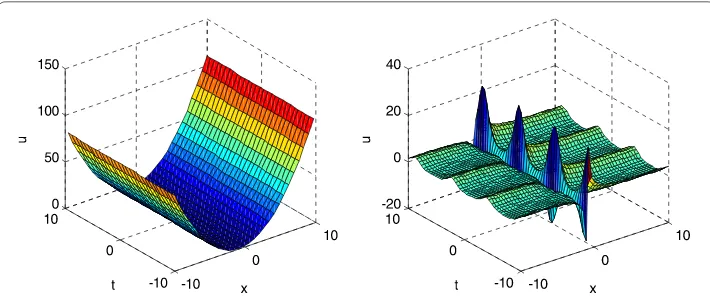
Figure 1Oscillatory soliton solution (left) and dark soliton solution (right) given by equation (3.16) withA= 1,

B= 1,a0=c0=d1= 1, andτ1(t) = exp(t) + sec(t) tan(t) +t

Case2:

a0=a0, b1= 1, c1=

2K4

K3

and

a1=a2=b2=c0=c2=d2=d2=K1=μ= 0.

(3.15)

Now, when we substitute equations (3.14), (3.15) and the solution of linear equation (3.10) forμ= 0 into equation (3.11), we get the solution of nonlinear equation (3.8). Fur-ther, using the value of solutionf(ξ) andg(ξ) into equation (3.7), we have rational solutions of equation (1.1) as follows.

Case1 gives the rational solution of equation (1.1) by the following relation:

u(x,t) =

τ1(t)dt

–1

a0+

B A+Bx

–1

,

w(x,t) =c0+d1

B A+Bx

–1

,

(3.16)

whereAandBare arbitrary constants (see Fig.1).

Similarly,Case2 gives the rational solution by the following relation:

u(x,t) =

τ1(t)dt

–1

a0+

B A+Bx

–1

,

w(x,t) =2K4

K3

B A+Bx

2

,

(3.17)

whereA,B,K3, andK4are arbitrary constants.

3.3 Subalgebra

Γ

λ

Γ

The solutions of system (1.1), which are invariant under this subalgebra with the coeffi-cient functions

τ2(t) =

K1

λ4

τ1(t)exp

–1

λ4

τ1(t)dt

, τ3(t) =

K2

λ4

κ1(t) =

are given by the following relations:

u(x,t) =f(ξ), expansion method. Therefore, following the procedure adopted in subalgebra3.2, we get

p= 2,q= 2. So we can suppose that the solution of ODEs (3.20) is of the form

Also, when we put (3.21) into the second equation of (3.20), it brings the system of al-gebraic equations as follows:

(i) 24b2K5μ3+ 2K3d22μ= 0,

(ii) 6d2K4μ2+ 6b1μ3K5+ 3K3μd1d2= 0,

(iii) 2d1K4μ2+ 40b2μ2K5+ 2c0μd2K3+K3d12μ+ 2K3d22= 0,

(iv) 8d2K4μ+ 8b1μ2K5+K3c0μd1+K3d2c1μ+ 3K3d1d2+d2= 0,

(v) 2d1K4μ+ 16b2μK5+ 2K3c0d2– 2K3d2c2μ+K3d21+ 2K3c2d2μ+d1= 0,

(vi) 2d2K4– 2a1μ2K5+ 2b1μK5–K3c0c1μ+K3c0d1+K3c1d2–K3d1c2μ

+ 2c2K4μ2+c0= 0, (3.23)

(vii) 2c1K4μ– 16a2μ2K5– 2K3c0c2μ–K3c21μ+c1= 0,

(viii) 8c2K4μ– 8a1μK5– 3K3c1c2μ–K3c0c1–K3c2d1+c2= 0,

(ix) 2c1K4– 40a2μK5– 2K3c0c2–K3c21– 2K3c22μ= 0,

(x) –6a1K5– 3K3c1c2+ 6K4c2= 0,

(xi) –24a2K5– 2K3c22= 0.

On solving algebraic equations (3.22) and (3.23) for arbitrary value ofK5, we get only

the trivial solutions of the main system (1.1), which is not a physically interesting case. Therefore, we reach the following results.

Case1:

a2=a2, c0=c0, d1= –

1

K3

, K2= –

1 12λ4a2,

a0=a1=b1=b2=c1=c2=d2=K5=μ= 0;

(3.24)

Case2:

a2= –

12K2

λ4

, c0=c0, d1= –

1

K3

, and

a0=a1=b1=b2=c1=c2=d2=K5=μ= 0.

(3.25)

Now when we substitute equations (3.24), (3.25) and the solution of linear equation (3.10) forμ= 0 into equation (3.21), we get the solution of nonlinear equation (3.20). Further, using the value of solutionf(ξ) andg(ξ) into equation (3.19), we have rational solutions of equation (1.1) as follows.

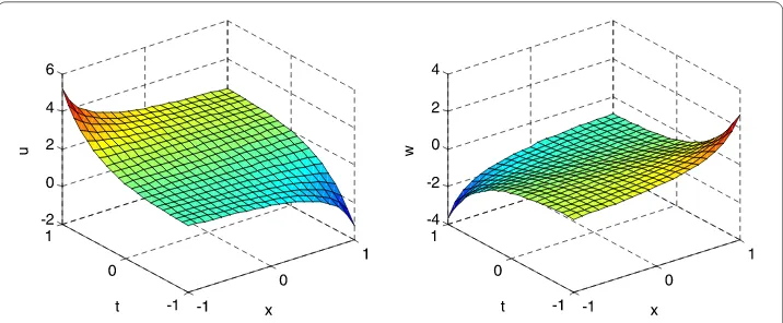
Case1 gives the rational solution of equation (1.1) by the following relation:

u(x,t) =a2

B A+Bx

2

,

w(x,t) =exp

1

λ4

τ1(t)dt

c0–

1

K3

B A+Bx

–1

,

(3.26)

Figure 2Smooth soliton solution (left) and breather soliton solution (right) given by equation (3.26) with

K3= –1,A=B= 1,a2=c0=λ4= 1, andτ1(t) = cos(t) + sin(t)

Similarly,Case2 gives the rational solution of equation (1.1) by the following relation:

u(x,t) = –12K2

λ4

A2

A1+A2x

2

,

w(x,t) =exp

1

λ4

τ1(t)dt

c0–

1

K3

A2

A1+A2x

–1

,

(3.27)

whereA,B,K2,K3, andλ4are arbitrary constants.

3.4 Subalgebra

Γ

Γ

The solutions of system (1.1) which are invariant under this subalgebra with the coefficient functions

τ2(t) =K1τ1(t), τ3(t) =K2τ1(t), κ1(t) =K3τ1(t),

κ2(t) =K4τ1(t), κ3(t) =K5τ1(t)

(3.28)

are given by the following relations:

u(x,t) =f(ξ),

w(x,t) =g(ξ),

(3.29)

whereξ=x–τ1(t)dtandf(ξ),g(ξ) are the solution of the system of nonlinear ordinary

differential equations

–f+ff+K1g+K2f= 0,

–g+K3gg+K4g+K5f= 0.

(3.30)

of ODEs (3.30) as follows:

f(ξ) =a0+a1

G(ξ)

G(ξ)

+a2

G(ξ)

G(ξ)

2

+b1

G(ξ)

G(ξ)

–1

+b2

G(ξ)

G(ξ)

–2

,

g(ξ) =c0+c1

G(ξ)

G(ξ)

+c2

G(ξ)

G(ξ)

2

+d1

G(ξ)

G(ξ)

–1

+d2

G(ξ)

G(ξ)

–2

.

(3.31)

By substituting (3.31) into the system of ODEs (3.30), using linear ODE (3.10), and equat-ing the coefficients of same powers of (G/G) to zero we obtain a set of simultaneous alge-braic equations amonga0,a1,a2,b1,b2,c0,c1,c2,d1,d2, andμas follows:

(i) 24b2K2μ3+ 2b22μ= 0,

(ii) 6d2K1μ2+ 6b1μ3K2+ 3μb1b2= 0,

(iii) 2d1K1μ2+ 40b2μ2K2+ 2a0μb2+b21μ+ 2b22– 2b2μ= 0,

(iv) 8d2K1μ+ 8b1μ2K2+a0μb1+b2a1μ+ 3b1b2–b1μ= 0,

(v) 2d1K1μ+ 16b2μK2+ 2a0b2– 2b2a2μ+b21+ 2a2b2μ– 2b2= 0,

(vi) 2d2K2– 2a1μ2K2+ 2b1μK2–a0a1μ+a0b1+a1b2–b1a2μ

+ 2c2K1μ2+a1μ–b1= 0, (3.32)

(vii) 2c1K1μ– 16a2μ2K2– 2a0a2μ–a21μ+ 2a2μ= 0,

(viii) 8c2K1μ– 8a1μK2– 3a1a2μ–a0a1–a2b1+a1= 0,

(ix) 2c1K1– 40a2μK2– 2a0a2–a21– 2a22μ+ 2a2= 0,

(x) –6a1K2– 3a1a2+ 6K1c2= 0,

(xi) –24a2K2– 2a22= 0.

Also, when we put (3.31) into the second equation of (3.30), it brings the system of al-gebraic equations as follows:

(i) 24b2K5μ3+ 2K3d22μ= 0,

(ii) 6d2K4μ2+ 6b1μ3K5+ 3K3μd1d2= 0,

(iii) 2d1K4μ2+ 40b2μ2K5+ 2c0μd2K3+K3d21μ+ 2K3d22– 2d2μ= 0,

(iv) 8d2K4μ+ 8b1μ2K5+K3c0μd1+K3d2c1μ+ 3K3d1d2–d1μ= 0,

(v) 2d1K4μ+ 16b2μK5+ 2K3c0d2– 2K3d2c2μ+K3d21+ 2K3c2d2μ– 2d2= 0,

(vi) 2d2K4– 2a1μ2K5+ 2b1μK5–K3c0c1μ+K3c0d1+K3c1d2–K3d1c2μ

+ 2c2K4μ2+c1μ–d1= 0, (3.33)

(vii) 2c1K4μ– 16a2μ2K5– 2K3c0c2μ–K3c21μ+ 2c2μ= 0,

(viii) 8c2K4μ– 8a1μK5– 3K3c1c2μ–K3c0c1–K3c2d1+c1= 0,

(ix) 2c1K4– 40a2μK5– 2K3c0c2–K3c21– 2K3c22μ+ 2c2= 0,

(xi) –24a2K5– 2K3c22= 0.

Similarly solving these algebraic equations as under the above subalgebras yields the following.

Now, when we substitute equations (3.34), (3.35) and the solution of linear equation (3.10) into equation (3.31), we get the solution of nonlinear equation (3.30). Further, using the value of solutionf(ξ) andg(ξ) into equation (3.29), we have hyperbolic, trigonometric, and rational function solutions of equation (1.1) as follows.

Case1:

Now, under Case 1 we haveμ= –₁₆1 c21

c2₂,i.e., (μ< 0), then the hyperbolic function solution of the main system (1.1) is given as follows:

w(x,t) = –1

c1= 0. Therefore, forμ= 0, we obtained the rational function solutions of equation (1.1)

as follows:

Ifμ> 0, the trigonometric function solution of the main equation (1.1) is given by the following relation:

whereA,B, andK4are arbitrary constants.

Ifμ< 0, then the hyperbolic function solution of the main system (1.1) is given as fol-lows:

Figure 3Kink compacton soliton solutions given by equation (3.40) witha1= 1,c1= –1,K4= –1,A=B= 1,

andτ1(t) = cosech2(t)

Whenμ= 0, we obtain the rational solution as follows:

u(x,t) = 1 +a1

B

A+B(x–τ1(t)dt)

,

w(x,t) = c1 2K4

+c1

B

A+B(x–τ1(t)dt)

,

(3.40)

whereA,B, andK4are arbitrary constants (see Fig.3).

4 Concluding and discussion

In this paper, the authors have studied new soliton solutions of time-dependent coupled KdV–Burgers equation with the help of two methods: the Lie symmetry group method and the modified (G/G)-expansion method. Thus, by the applications of Lie symmetry method, we have reduced nonlinear PDEs (1.1) to the system of nonlinear ODEs under different subalgebras. The reduced nonlinear ODEs are highly nonlinear, which is difficult to solve analytically. Therefore, in the quest of solutions for the reduced nonlinear ODEs, we take the help of a novel method called (G/G)-expansion method. The physical behav-iors of the obtained solutions are represented with the help of Fig.1, Fig.2, and Fig.3.

Funding

This research was funded by the Deanship of Scientific Research at Princess Nourah bint Abdulrahman University through the Fast-track Research Funding Program.

Competing interests

The authors declare that they have no conflicts of interest to this work. There is no professional or other personal interest of any nature or kind in any product that could be construed as influencing the position presented in the manuscript entitled.

Authors’ contributions

All authors read and approved the final manuscript.

Author details

1_{Department of Mathematical Sciences, College of Sciences, Princess Nourah bint Abdulrahman University, Riyadh, Saudi}

Arabia. 2_{Department of Mathematics, D.A.V. College Pundri, Kaithal, India.}

Publisher’s Note

Springer Nature remains neutral with regard to jurisdictional claims in published maps and institutional affiliations.

References

1. Su, C.H., Gardner, C.S.: Derivation of the Korteweg–de Vries and Burgers’ equation. J. Math. Phys.10, 536–539 (1969) 2. Helfrich, K.R., Melville, W.K., Miles, J.W.: On interfacial solitary waves over variable topography. J. Fluid Mech.149,

305–317 (1984)

3. Korteweg, D.J., Vries, G.: On the change of form of long waves advancing in a rectangular canal, and on a new type of long stationary waves. Philos. Mag.39, 422–443 (1895)

4. Wijngaarden, L.V.: On the motion of gas bubbles in a perfect fluid. Annu. Rev. Fluid Mech.4, 369–373 (1972) 5. Johnson, R.S.: Shallow water waves on a viscous fluid—the undular bore. Phys. Fluids15, 1693–1699 (1972) 6. Burgers, J.M.: A Mathematical Model Illustrating the Theory of Turbulence. Adv. Appl. Mech. Academic Press, New

York (1948)

7. Hu, P.N.: Collisional theory of shock and nonlinear waves in a plasma. Phys. Fluids15, 854–864 (1972)

8. Mowafy, A.E., El-Shewy, E.K., Moslem, W.M., Zahran, M.A.: Effect of dust charge fluctuation on the propagation of dust-ion acoustic waves in inhomogeneous mesospheric dusty plasma. Phys. Plasmas15, 073708 (2008) 9. Johnson, S., Suarez, P., Biswas, A.: New exact solutions for the sine-Gordon equation in (2 + 1)-dimensions. Comput.

Math. Math. Phys.52, 98–104 (2012)

10. Peng, X.X., Qian, M., Yong, C.: Nonlocal symmetries and exact solutions for PIB equation. Commun. Theor. Phys.58, 331–337 (2012)

11. Ashyralyeva, A., Koksal, M.E.: On the second order of accuracy difference scheme for hyperbolic equations in a Hilbert space. Numer. Funct. Anal. Optim.26, 739–772 (2006)

12. Kumar, H., Malik, A., Chand, F.: Soliton solutions of some nonlinear evolution equations with time-dependent coefficients. Pramana J. Phys.80, 361–367 (2013)

13. Olver, P.J.: Applications of Lie Groups to Differential Equations. Graduate Texts Math. Springer, New York (1993) 14. Ovsiannikov, L.V.: Group Analysis of Differential Equations. Academic Press, New York (1982)

15. Bluman, G.W., Kumei, S.: Symmetries and Differential Equations. Springer, New York (1989) 16. Chou, T.: Lie Group and Its Applications in Differential Equations. Science Press, Beijing (2001)

17. Kaur, L., Gupta, R.K.: Kawahara equation and modified Kawahara equation with time dependent coefficients: symmetry analysis and generalized (G/G)-expansion method. Math. Methods Appl. Sci.36, 584–601 (2013) 18. Papamikos, G., Pryer, T.: A Lie symmetry analysis and explicit solutions of the two dimensional_∞-polylaplacian. Stud.

Appl. Math.142, 48–64 (2018)

19. Johnpillai, A.G., Kara, A.H., Biswas, A.: Symmetry reduction, exact group-invariant solutions and conservation laws of the Benjamin–Bona–Mahoney equation. Appl. Math. Lett.26, 376–381 (2013)

20. Kumar, V., Gupta, R.K., Jiwari, R.: Painlevé analysis, Lie symmetries and exact solutions for variable coefficients Benjamin–Bona–Mahony–Burger (BBMB) equation. Commun. Theor. Phys.60, 175–182 (2013)

21. Kumar, V., Kaur, L., Kumar, A., Koksal, M.E.: Lie symmetry based-analytical and numerical approach for modified Burgers–KdV equation. Results Phys.8, 1136–1142 (2018)

22. Yunqing, Y., Yong, C.: Prolongation structure of the equation studied by Qiao. Commun. Theor. Phys.56, 463–466 (2011)

23. Ablowitz, M.J., Clarkson, P.A.: Solitons, Nonlinear Evolution Equations and Inverse Scattering Transform. Cambridge University Press, Cambridge (1991)

24. Cariello, F., Tabor, M.: Similarity reductions from extended Painlevé expansions for nonintegrable evolution equations. Physica D53, 59–70 (1991)

25. Liu, S.K., Fu, Z.T., Liu, S.D., Zhao, Q.: Jacobi elliptic function expansion method and periodic wave solutions of nonlinear wave equations. Phys. Lett. A289, 69–74 (2001)

26. Kumar, H., Chand, F.: Applications of extended F-expansion and projective Ricatti equation methods to (2 + 1)-dimensional soliton equations. AIP Adv.3, 032128 (2013)

27. He, J.H., Wu, X.H.: Exp-function method for nonlinear wave equations. Chaos Solitons Fractals30, 700–708 (2006) 28. Wang, M.L., Li, X., Zhang, J.: The (G/G)-expansion method and travelling wave solutions of nonlinear evolution

equations in mathematical physics. Phys. Lett. A372, 417–423 (2008)

29. Miao, X., Zhang, Z.: The modified (G/G)-expansion method and traveling wave solutions of nonlinear perturbed Schrodinger’s equation with Kerr law nonlinearity. Commun. Nonlinear Sci. Numer. Simul.16, 4259–4267 (2011) 30. Malik, A., Kumar, H., Chand, F., Mishra, S.C.: Exact traveling wave solutions of the Bogoyavlenskii equation using

multiple (G/G)-expansion method. Comput. Math. Appl.64, 2850–2859 (2012)

31. Bansala, A., Gupta, R.K.: Modified (G/G)-expansion method for finding exact wave solutions of the coupled Klein–Gordon–Schrödinger equation. Math. Methods Appl. Sci.35, 1175–1187 (2012)

32. Whitham, G.B.: Linear and Nonlinear Waves. Academic Press, New York (1973)

33. Wang, M.L.: Exact solutions for a compound KdV–Burgers equation. Phys. Lett. A213, 279–287 (1996)

34. Shaojie, Y., Cuncai, H.: Lie symmetry reductions and exact solutions of a coupled KdV–Burgers equation. Appl. Math. Comput.234, 579–583 (2014)

35. Drazin, P., Johnson, R.: Solitons: An Introduction. Cambridge Univesity Press, New York (1989)

36. Kumar, V., Alqahtani, A.: Lie symmetry analysis, soliton and numerical solutions of boundary value problem for variable coefficients coupled KdV–Burgers equation. Nonlinear Dyn.90, 2903–2915 (2017)

37. Singh, K., Gupta, R.K.: Lie symmetries and exact solutions of a new generalized Hirota–Satsuma coupled KdV system with variable coefficients. Int. J. Eng. Sci.44, 241–255 (2006)

38. Vaneeva, O.O., Papanicolaou, N.C., Christou, M.A., Sophocleous, C.: Numerical solutions of boundary value problems for variable coefficient generalized KdV equations using Lie symmetries. Commun. Nonlinear Sci. Numer. Simul.19, 3074–3085 (2014)