Volume 2008, Article ID 367287,10pages doi:10.1155/2008/367287
Research Article
Differentially Encoded LDPC Codes—Part II:
General Case and Code Optimization
Jing Li (Tiffany)
Electrical and Computer Engineering, Lehigh University, Bethlehem, PA 18015, USA
Correspondence should be addressed to Jing Li (Tiffany),[email protected]
Received 19 November 2007; Accepted 6 March 2008
Recommended by Yonghui Li
This two-part series of papers studies the theory and practice of differentially encoded low-density parity-check (DE-LDPC) codes, especially in the context of noncoherent detection. Part I showed that a special class of DE-LDPC codes, product accumulate codes, perform very well with both coherent and noncoherent detections. The analysis here reveals that a conventional LDPC code, however, is not fitful for differential coding and does not, in general, deliver a desirable performance when detected noncoherently. Through extrinsic information transfer (EXIT) analysis and a modified “convergence-constraint” density evolution (DE) method developed here, we provide a characterization of the type of LDPC degree profiles that work in harmony with differential detection (or a recursive inner code in general), and demonstrate how to optimize these LDPC codes. The convergence-constraint method provides a useful extension to the conventional “threshold-constraint” method, and can match an outer LDPC code to any given inner code with the imperfectness of the inner decoder taken into consideration.
Copyright © 2008 Jing Li (Tiffany). This is an open access article distributed under the Creative Commons Attribution License, which permits unrestricted use, distribution, and reproduction in any medium, provided the original work is properly cited.
1. INTRODUCTION
With an increasingly mature status of the sparse-graph coding technology in a theoretical context, the very pervasive scope of their well-proven practical applications, and the wide-scale availability of software radio, low-density parity-check (LDPC) codes have become and continue to be a favorable coding strategy for researchers and practitioners. Their superb performance on various channel models and with various modulation schemes have been documented in many papers. While the existing literature has shed great light on the theory and practice of LDPC codes, investigation was largely carried out from a pure coding perspective, where the prevailing assumption is that the synchronization and channel estimation are handled perfectly by the front-end receiver.
In wireless communications, accurate phase estimation may in many cases be very expensive or infeasible, which calls for noncoherent detection. Practical noncoherent detection is generally performed in one of the two ways: inserting pilot symbols directly in the coded and modulated sequence to help track the channel (it is possible to insert either pilot tones or pilot symbols, but the latter is found to be
more effective and is what of relevance to this paper), and employing differential coding. Considering that the former may result in a nontrivial expansion of bandwidth especially on fast-changing channels, many wireless systems adopt the latter, including satellite and radio-relay communications.
The problem we wish to investigate is: LDPC codes perform remarkably well with coherent detection, but how about their performance with noncoherent detection and noncoherent differential detection in particular? This series of two-part papers aim to generate useful insight and engineering rules. In Part I of the series [1], we considered a special class of differentially encoded LDPC (DE-LDPC) codes, product accumulate (PA) codes [2]. The outer code of a (p(t+ 2),pt) PA code is a simple, structured LDPC code with left (variable) degree profileλ(x)=1/(t+ 1) +t/(t+ 2)x and right (check) degree profileρ(x)=xt; and the inner code
interesting problems. For example, what is the best strategy to apply LDPC codes in noncoherent detection—should differential coding be used or not? Modulation schemes such as the minimum phase shift keying (MPSK) have equivalent realizations in recursive and non-recursive forms; is one form preferred over the other in the context of LDPC coding? What other DE-LDPC configurations, besides PA codes, are good for differential coding, and how to find them?
Since the conventional differential detector (CDD) oating on two symbol intervals incurs a nontrivial per-formance loss [7], and since multiple symbol differential detectors (MSDD) [8] have a rather high complexity that increases exponentially with the window size, we developed, in Part I of this series of papers, a simple iterative differential detection and decoding (IDDD) receiver, whose structure is shown in [1, Figure 6]. The IDDD receiver comprises a CDD with 2-symbol observation window (the current and the previous), a phase-tracking Wiener filter, a message-passing decoder for the accumulator 1/(1 +D) [2], and a message-passing decoder configured for the (outer) LDPC code. The CDD, coupled with the phase-tracking unit and the 1/(1 + D) decoder, acts as the front-end, or, the inner decoder of the serially concatenated system, and the succeeding LDPC decoder acts as the outer decoder. Soft reliability information in the form of log-likelihood ratio (LLR) is exchanged between the inner and the outer decoders to successively refine the decision. In the sequel, unless otherwise stated, we take the IDDD receiver as the default noncoherent receiver in our discussion of DE-LDPC codes.
We study the convergence property of IDDD for a general DE-LDPC code, through extrinsic information transfer (EXIT) charts [9,10]. A somewhat unexpected finding is that, while ahigh-ratePA code yields desirable performance with noncoherent (differential) detection, a general DE-LDPC code does not. We attribute the reason to the mis-match of the convergence behavior between a conventional LDPC code and a differential decoder. This suggests that conventional LDPC codes, while an excellent choice for coherent detection, are not as desirable for noncoherent detection. It also gives rise to the question of what special LDPC codes, possibly performing poorly in the conventional scenario (such as the outer code of the PA code), may turn out right for differential modulation and detection?
One remarkable property of LDPC codes is the possibil-ity to design their degree profiles, through denspossibil-ity evolution [11], to match to a specific channel or a specific inner code [12–15]. To make LDPC codes work in harmony with the noncoherent differential decoder of interest, here we develop
a convergence-constraint density evolution method. The
conventionalthreshold-constraintmethod [11,16] targets the best asymptotic threshold, and the new method effectively captures the interaction and convergence between the inner and the outer EXIT curves through a set of “sample points.” In that, it makes it possible to optimize LDPC codes to match to an (arbitrary) inner code/modulation with the imperfectness of the inner decoder/demodulator taken into account. Our study reveals that LDPC codes may be divided in two groups. Those having minimum left degree of≥2 are generally suitable for a nonrecursive inner code/modulator
but not for a differential detector or any recursive inner code. On the other hand, the LDPC codes that perform well with a recursive receiver always have degree-1 (and degree-2) variable nodes. Further, when the code rate is high, these degree-1 and -2 nodes become dominant. This also explains why high-rate PA codes, whose outer code has degree-1 and degree-2 nodes only, perform remarkably with (noncoherent) differential detection [1].
The channel model of interest here is flat Rayleigh fading channels with additive white Gaussian noise (AWGN), the same as discussed in Part I [1]. Letrkbe the noisy signal at
the receiver, let sk be the binary phase shift keying (BPSK)
modulated signal at the transmitter, let nk be the i.i.d.
complex AWGN with zero mean and varianceσ2 =N 0/2 in
each dimension, and letαkejθkbe the fading coefficient with
Rayleigh distributed amplitudeαkand uniformly distributed
phaseθk. We haverk=αkejθksk+nk. Throughout the paper,
θk is assumed known perfectly to the receiver/decoder in
the coherent detection case, and unknown (and needs to be worked around) in the noncoherent detection case. Further, the receiver is said to have channel state information (CSI) if αkknown (irrespective ofθk), and no CSI otherwise.
We consider correlated channel fading coefficients (so that noncoherent detection is possible). Applying Jakes’ isotropic scattering land mobile Rayleigh channel model, the autocorrelation ofαkis characterized by the 0th-order Bessel
function of the first kind
Rk=
1
2J0(2kπ fdTs), (1) and the power spectrum density (PSD) is given by
S(f)= P π
1−f / fd
2, for|f|< fd, (2)
where fdTs is the normalized Doppler spread, f is the
frequency band,τ is the lag parameter, andP is a constant that is dependent on the average received power given a specific antenna and the distribution of the angles of the incoming power.
The rest of the paper is organized as follows.Section 2 evaluates the performance of a conventional LDPC code with noncoherent detection, and compare it with that of PA codes. Section 3 proposes the convergence-constraint method to optimize LDPC codes to match to a given inner code and particular a differential detector. Section 4 concludes the paper.
2. CODES MATCHED TO DIFFERENTIAL CODING
Part I showed that PA codes, a special class of DE-LDPC codes, perform quite well with coherent detection as well as noncoherent detection [1]. This section reveals whether or not this also holds for general DE-LDPC codes, and the far subtly why.
recent studies have revealed surprisingly elegant and useful properties of EXIT charts. Specifically, theconvergence prop-ertystates that, in order for the iterative decoder to converge successfully, the outer EXIT curve should stay strictly below the inner EXIT curve, leaving an open tunnel between the two curves. The area property states that the area under the EXIT curve, A = 10IedIa, corresponds to the rate of
the code [10], whereIa andIe denote the a priori (input)
mutual information to and the extrinsic (output) mutual information from a particularly subdecoder, respectively. When the auxiliary channel is an erasure channel and the subdecoder is an optimal one, the relation is exact; otherwise, it is a good approximation [10]. The immediate implication of these properties is that, to fully harness the capacity (achievable rate) provided by the (noncoherent) inner differential decoder, the outer code must have an EXIT curve closely matchedin shape and in positionto that of the inner code.
With this in mind, we evaluate a few examples of (DE-)LDPC codes. (The computation of EXIT charts specific to DE-LDPC codes with IDDD receiver is discussed in [1].) We consider two configurations of the inner code:
(1) a differential decoder for 1/(1 +D); and (2) a direct detector, that is, a BPSK detector;
and three configurations of the outer code:
(1) the outer code of a PA code, which has degree profile:
λ(x)=1 7+
6 7x, ρ(x)=x7;
(3)
(2) a (3,12)-regular LDPC code; and
(3) an optimized irregular LDPC code reported in [17], whose threshold is 0.6726—about 0.0576 dB away from the AWGN capacity—and whose degree profile is
γ(x)=0.1510x+0.1978x2+0.2201x6+0.03537+0.3958x29,
ρ(x)=x20.
(4)
All three outer codes have rate 3/4, and the channel is a correlated Rayleigh fading channel with AWGN and normalized Doppler rate of fdTs=0.01.
The EXIT curves, plotted inFigure 1, demonstrate that the outer code of the PA code and the differential decoder match quite well, but a conventional LDPC code, regular or irregular, will either intersect with the differential decoder, causing decoder failure, or leave a huge area between the curves, causing a capacity loss. On the other hand, LDPC codes, especially the (optimized) irregular ones, agree very well with the direct detector. This suggests that (conventional) LDPC codes perform better as a single code than being concatenated with a recursive inner code. Put it another way, an LDPC code that is optimal in the usual sense, for example, BPSK modulation and memoryless channels, may become quite suboptimal when operated together with a recursive inner code or a recursive modulation, such
1 0.9 0.8 0.7 0.6 0.5 0.4 0.3 0.2 0.1 0 Ie,i
/Ia
,
o
0 0.2 0.4 0.6 0.8 1
Ia,i/Ie,o 0.35
0.29 0.24
0.19 0.15
0.12 0.085
0.055 0.026
0.013 0.0025 0.005 0.0076
fdTs=0.01,Eb/N0=5.32,R=3/4
Differential code 1/(1 +D) Fading channel
Outer code of PA code
LDPC code (regular) LDPC code (irregular) Regular LDPC
Irregular LDPC PA (outer) Rayleigh channel
Differential code
Figure1: EXIT curves of LDPC codes, the outer code of PA codes, differential decoder and the direct detector of Rayleigh channels. Normalized Doppler rate 0.01, Eb/N0 = 5.32 dB, code rate 3/4,
(3, 12)-regular LDPC code, and optimized irregular LDPC code withρ(x)=x20andγ(x)=0.1510x+0.1978x2+0.2201x6+0.03537+
0.3958x29.
as a differential encoder. On the other hand, not using differential coding generally requires more pilot symbols in order to track the channel well, especially on fast-fading environments. Hence, it is fair to say that (conventional) LDPC codes that boast outstanding performance under coherent detection may not be nearly as advantageous under noncoherent detection, since they either suffer from performance loss (with differential encoding) or incur a large bandwidth expansion (without differential encoding). In comparison, PA codes can make use of the (intrinsic) differential code for noncoherent detection, and therefore present a better choice for bandwidth-limited wireless appli-cations.
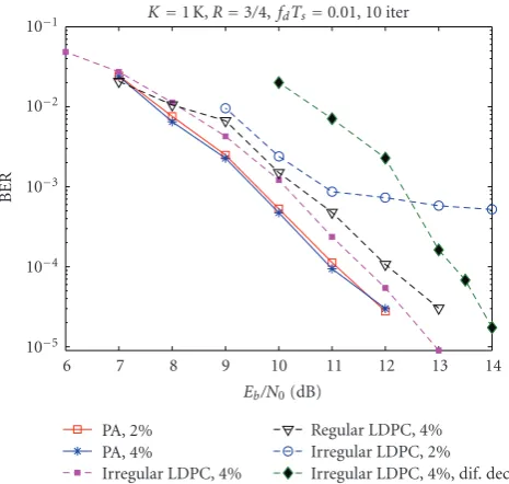
Figure 2plots the BER performance curves of the same three codes specified inFigure 1on Rayleigh channels with noncoherent detection. All the codes have data block size K = 1 K and code rate 3/4. Soft feedback is used in IDDD, the normalized Doppler spread is 0.01, and 2% or 4% pilot symbols are inserted to help track the channel. The two LDPC codes are evaluated either with or without a differential inner code. From the most power efficient to the least power efficient, the curves shown are (i) PA code with 4% of pilot symbols, (ii) PA code with 2% of pilot symbols, (iii) BPSK-coded irregular LDPC code with 4% of pilot symbols, (iv) BPSK-coded regular LDPC code with 4% of pilot symbols, (v) BPSK-coded irregular LDPC code with 2% of pilot symbols, (vi) differentially encoded irregular LDPC code with 4% of pilot symbols. It is evident that (conventional) LDPC codes suffer from a differential inner code. For example, with 4% of bandwidth expansion, BPSK-coded irregular and regular LDPC codes perform about 0.5 and 1 dB worse than PA codes at BER of 10−4, respectively, but the differentially encoded irregular LDPC code falls short by more than 2.2 dB. Further, while the irregular LDPC code (not differentially coded) is moderately (0.5 dB) behind the PA code with 4% of pilot symbols, the gap becomes much more significant when pilot symbols are reduced in half. For PA codes, 2% of pilot symbols remain adequate to support a desirable performance, but they become insufficient to track the channel for nondifferentially encoded LDPC codes, causing a considerable performance loss and an error floor as high as BER of 10−3. Thus, the
advantages of PA codes over (conventional) LDPC codes are rather apparent, especially in cases when noncoherent detection is required and when only limited bandwidth expansion is allowed.
3. CODE DESIGN FROM THE CONVERGENCE PROPERTY
3.1. Problem formulation
EXIT analysis and computer simulations in the previous section show that a conventional LDPC code does not fit differential coding, but special cases such as the the outer code of PA codes do. This raises more interesting questions: what other (special) LDPC codes are also in harmony with differential encoding? What degree profiles do they have? Is it possible to characterize and optimize the degree profiles, and how?
The fundamental tool to solve these questions lies in convex optimization. In [11], the optimization problem of the irregular LDPC degree profiles on AWGN channels was formulated as a duality-based convex optimization problem, and an iterative method termed density evolution was proposed to solve the problem. In [16], a Gaussian approximation was applied to the density evolution method, which reduces the problem to be a linear optimization problem. Density evolution has since been exploited, in different flavors and possibly combined with differential evolution [18], to design good LDPC ensembles for a vari-ety of communication channels and modulation schemes,
10−1
10−2
10−3
10−4
10−5
BER
6 7 8 9 10 11 12 13 14
Eb/N0(dB)
K=1 K,R=3/4,fdTs=0.01, 10 iter
PA, 2% PA, 4%
Irregular LDPC, 4%
Regular LDPC, 4% Irregular LDPC, 2% Irregular LDPC, 4%, dif. dec.
Figure2: Comparison of PA codes and LDPC codes on fast-fading Rayleigh channels with noncoherent detection and decoding. Solid line: PA codes, dashed lines: LDPC codes. Code rate 0.75, data block size 1 K, filter length 65, normalized Doppler spread 0.01, 10 global iterations, and 4 (local) iterations within LDPC codes or the outer code of PA codes inside each global iteration.
see, for example [12–15] and the references therein. The results reported in these previous papers are excellent, but they almost exclusively aimed at the asymptotic threshold, namely, their cost functions were set to minimize the SNR threshold for a target code rate, or, equivalently, to maximize the code rate for a target SNR threshold. This is well justified, since in these papers, the primary involvement of the channel is to provide the initial LLR information to trigger the start of the density evolution process.
However, the problem we consider here is somewhat different. Our goal is to design codes that can fully achieve the capacity provided by the given inner receiver, and the noncoherent differential decoder in particular. Considering that the inner receiver, due to the lack of channel knowledge or other practical constraints, may not be an optimal receiver, it is of paramount importance to control the interaction between the inner and the outer code, or, the convergence behavior as reflected in the matching of shape and position of the corresponding EXIT curves. To emphasize the difference, we thereafter refer to the conventional density evolution method as the “threshold-constraint” method, and propose a “convergence-constraint” method as a useful extension to the conventional method.
The key idea of the proposed method is to sample the inner EXIT curve and design an (outer) EXIT curve that matches with these sample points, or, “control points.” Suppose we choose a set ofM control points in the EXIT plane, denoted as (v1,w1), (v2,w2),. . ., (vM,wM). Let To(·)
will be defined later in (17)), the optimization problem is
whereRdenotes the code rate of the outer LDPC code, and λiandρidenote the fraction of edges that connect to variable
nodes and check nodes of degreei, respectively.
The formulation in (5) assumes that the LLR mes-sages at the input of the inner and the outer decoder are Gaussian distributed, and that the output extrinsic mutual information (MI) of an irregular LDPC code corresponds to a linear combination of the extrinsic MI from a set of regular codes. As reported in literature, the Gaussian assumption for LLR messages is less not far from reality on AWGN channels but less accurate on Rayleigh fading channels [12]. Nevertheless, Gaussian assumption is used for several reasons. The first reason is simplicity and tractability. Tracking and optimizing the exact message pdf ’s involves tedious computation, which is exacerbated by the fact the proposed new method is governed by a set of control points, rather than a single control point as in the conventional method. Second, recall that to compute EXIT curves inevitably uses the Gaussian approximation. Thus, it seems well acceptable to adopt the same approximation when shaping and positioning an EXIT curve. Finally, characterizing and representing EXIT curves using mutual information help stabilize the process and alleviate the inaccuracy caused by Gaussian approxi-mation and other factors. As confirmed by many previous papers as well as this one, the optimization generates very good results in spite of the use of the Gaussian approxima-tion.
3.2. The optimization method
Below we detail the convergence-constraint design method formulated in (5). We conform to the notations and the graphic framework presented in [16]. Letλ(x)=Dv
i=1λixi−1
andρ(x)=Dc
i=2ρixi−1be the degree profiles from the edge
perspective, where Dv and Dc are the maximum variable
node and check node degrees, andλiandρiare the fraction
of edges incident to variable nodes and check nodes of degree i. Similarly, letλ(x)=Dv
i=1λixi−1andρ(x)= Dc
i=2ρixi−1be
the degree profiles from the node perspective. LetRbe the code rate. The following relation holds:
λi=
Let superscript (l) denote thelth LDPC decoding iteration, and subscript v andc denote the quantities pertaining to variable nodes and check nodes, respectively. Further, define
two functions that will be useful in the discussion
I(x)=1−
Function I(x) maps the message mean x to the corre-sponding mutual information (under Gaussian assumption), andφ(x) helps describe how the message mean evolves in tanh(y/2) operation, whereyfollows a Gaussian distribution with meanxand variance 2x.
The complete design process takes a dual constraint optimization process that progressively optimizes variable node degree profileλ(x) and check node degree profileρ(x) based on each other. Despite the duality in the formulation and the steps, optimizing λ(x) is far more critical to the code performance than optimizingρ(x), largely because the optimal check node degree profile are shown to follow the concentration rule [16]:
ρ(x)=Δxk+ (1−Δ)xk+1. (9)
It is therefore a common practice to presetρ(x) according to (9) and code rateR, and optimizeλ(x) only. For this reason, below we focus our discussion on optimizingλ(x) for a given ρ(x). Interested readers can formulate the optimization of ρ(x) in a similar way.
3.2.1. Threshold-constraint method (optimizingλ(x))
Under the assumption that the messages passed along all the edges are i.i.d. and Gaussian distributed, the average messages variable nodes receive from their neighboring check nodes follow a mixed Gaussian distribution. From (l−1)th iteration tolth local iteration (in the LDPC decoder), the mean of the messages associated with the variable node, mv, evolves as
wherem0 denotes the mean of the initial messages received
from the inner code (or the channel). Let us define
hi(m0,r)=Δφ
Then (11) can be rewritten as
The conventional threshold-constraint density evolution guarantees that the degree profile converges asymptotically to the zero-error state at the given initial message meanm0.
This is achieved by enforcing [16]
r > hm0,r
, ∀r∈0,φm0
. (14)
Viewed from the EXIT chart, the threshold-constraint method has implicitly used a control point (v,w) = (1, I(m0)), such that the resultant EXIT curve will stay below
it.
3.2.2. Convergence-constraint method (optimizingλ(x))
The proposed convergence-constraint method extends the conventional threshold-constraint method by introducing a set of control points, which may be placed in arbitrary positions in the EXIT plane, to control the shape and the position of the EXIT cure. Each control point (v,w) ∈ [0, 1]2ensures that the EXIT curve will, at the inputa priori
mutual informationw, produce extrinsic mutual informa-tion greater than v. This is reflected in the optimization process by changing (14) to
r∗> hm0,r∗
We can reformulate the problem as follows: for a given check node degree profile ρ(x) and a control point (v,w) in the EXIT chart, where 0≤v,w,≤1, to that of the conventional threshold-constraint design.
Hence, given a set of M control points, (v1,w1),
(v2,w2),. . ., (vM,wM), where 0 ≤v1 < v2 <· · · < vM ≤1
and 0 ≤ w1 ≤ w2 ≤ · · · ≤ wM ≤ 1, one can combine
the constraints associated with each individual control point and perform joint optimization, to control the shape and the position of the resulting EXIT curve. Specifically, when the set of control points are proper samples from the inner EXIT curve, the resultant EXIT curve represents an optimized LDPC ensemble that matches to the inner code.
3.2.3. Linear programming
The basic idea of convergence-constraint design, as discussed before, is simple. Complication arises from the fact that constraint (ii) in (16) is a nonlinear function ofλi’s.
Further-more, observe that the determination of the optimization range, or, the computation of r∗ from (17), requires the knowledge ofλ(x), which is yet to be optimized. One possible approach to overcome this chicken-and-egg dilemma is to attempt an approximated λ(x) in (17) to compute r∗. Specifically, we propose accounting for the two lowest degree variable nodes λi1 and λi2, and approximating the degree
profile as
in (17). First, this approximatedλ(x) is only used in (17) to tentatively determine r∗, so that the optimization process can get started. The exact λ(x) in (16), (i) and (ii), is to be optimized. Second, the value ofi1andλi1(orλ
i1) in the
approximatedλ(x) is calculated in one of the following two ways.
Case 1. A conventional LDPC ensemble hasi1 = 2, that is,
no degree-1 variable nodes. This is because the outbound messages from degree-1 variable nodes do not improve over the message-passing process. In that case, we consider only degree-2 and 3 nodes (λi1=2 and λi2=3), upper bound the
percentage of degree-2 nodes withλ∗2, and treat all the rest
as degree-3 nodes. The stability condition [11, 16] states that there exists a value ξ > 0 such that, given an initial symmetric message densityP0 satisfying
0
−∞P0(x)dx < ξ,
then the necessary and sufficient condition for the density evolution to converge to the zero-error state isλ(0)ρ(1)< eγ, whereγ= −Δ log(∞
−∞P0(x)e−x/2dx). Applying the stability
condition on Gaussian messages with initial mean value m0, we getγ = m0/4 and λ∗2 = em0/4/
It should be noted that not all values of wk from
the M preselected control points are suitable for (19) in computing λ∗2. Since the stability condition ensures the
asymptotic convergence to the zero-error state for a given input messages, λ2 ≤ λ∗2(w∗) is valid and required only
when the output mutual information will approach 1 at the input mutual informationw∗. What this implies in sampling the inner EXIT curve is that, at least one control point, say, the rightmost point (vM,wM), should roughly satisfy the
requirement: (vM,wM)≈ (1,wM). This value ofwM is then
used in (19) to computeλ∗2 =λ∗2(wM), which is subsequently
used inλ(x) ≈λ∗2x+ (1−λ∗2)x2to computer∗from (17).r∗
Checks Bits Checks Bits
Error
Error
LDPC Differential encoder
p
q
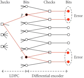
Figure3: Defect forλ1>1−R. When the four bits associated with
the solid circles flip altogether, another valid codeword results, and the decoder is unable to tell (undetectable error).
It is also worth mentioning that when a Gaussian approximation is used on the message pdf ’s, the stability condition reduces to
λ∗2(w)=
eI−1(w)/4
Dc
j=2(j−1)ρj
, (20)
which is a weaker condition than (19). Since we use Gaussian approximation primarily for the purpose of complexity reduction, unnecessary application is therefore avoided. Thus (19) rather than (20) is used in our design process.
Case 2. Consider the case when an LDPC code is iteratively
decoded together with a differential encoder, or, other recursive inner code or modulation with memory. Since the inner code imposes another level of checks on all the variable nodes, degree-1 variable nodes in the outer LDPC code will get extrinsic information from the inner code, and their estimates will improve with decoding iterations. Thus, without loss of generality, we let the first and the second nonzero λi’s be λ1 and λ2. No analytical bounds onλ1 or
λ2 were reported in literature for this case. We propose to
boundλ1byλ1 ≤1−R, whereRis the code rate (the exact
code rate is dependent on the optimization result, and may be slightly different from the target code rate). The rational is that, if λ1 > 1−R, then there exist at least two
degree-1 variable nodes, say the pth node and theqth node, which connect to the same check. When the LDPC code operates alone, these two variable nodes are apparently useless and wasteful, and can be removed altogether. When the LDPC code is combined with an inner recursive code, as shown in Figure 3, these two degree-1 variable nodes will cause a minimum distance of 4 for the entire codeword, irrespective of the code length. Using this empirical bound onλ1, we can
employ the approximationλ(x) =(1−R)+Rxin (17), which leads to the computation of (a lower bound for)r∗. Code optimization as formulated by the convergence-constraint method can thus be solved using linear programming.
It is rather expected that the choice of the control points directly affects the optimization results. The set of control
points need not be large—in fact, an excessive number of control points actually makes the optimization process con-verge slow and at times concon-verge poor. We suggest choosing 3 to 5 control points that can reasonably characterize the shape of the inner EXIT curve. Our experiments show that the proposed method generates EXIT curves with a shape matching very well to what we desire, but the position is slightly lower, indicating that the resultant code rate is slightly pessimistic. This can be compensated by presetting the control points slightly higher than we actually want them to be.
3.3. Optimization results and useful findings
For complexity concerns, instead of performing dual opti-mization, we apply the concentration theorem in (9) and preselectρ(x) that will make the the average column weight to be approximately 3. The left degree profileλ(x) is opti-mized through the convergence-constraint method discussed in the previous subsection. We now discuss some observa-tions and findings from our optimization experiments.
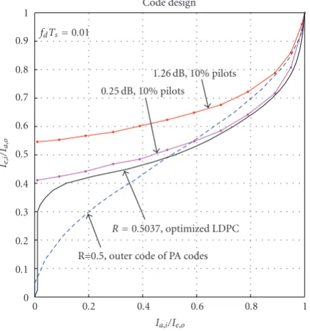
First, the LDPC ensemble optimal for differential coding always contains degree-1 and degree-2 variable nodes. For high rate codes above 0.75, these nodes are dominant, and in some cases, are the the only types of variable nodes in the degree profile. For medium rates around 0.5, there exist also a good portion of high-degree variable nodes. Considering that the outer code of a PA code has only degree-1 and degree-2 variable nodes,λ(x)=(1−R)/(1 +R) + (2R/(1 + R))x, where R ≥ 1/2 is the code rate, it is fair to say that PA are (near-)optimal at high rates, but less optimal at medium rates (the optimized LDPC ensemble contains slightly different degree distribution than that of the PA code, the difference is very small in either asymptotic thresholds or finite length simulations). This is actually well reflected in the EXIT charts. As rate 3/4 (seeFigure 1), the area between the outer code of the PA code and the inner differential code is very small, leaving not much room for improvement. In comparison, at rate around 0.5 (seeFigure 4), the area becomes much bigger, indicating that an optimized outer code could acquire more information rate for the same SNR threshold, or, for the same information rate, achieve a better SNR threshold.
The optimization result of a target rate 0.5 is shown in Figure 4. We consider an inner differential code, operating at 0.25 dB on a fdTs = 0.01 Rayleigh fading channel, and
decoded using the noncoherent IDDD receiver with the help of using 10% pilot symbols. The optimzed LDPC ensemble has code rateR=0.5037 and degree profile
λ(x)=0.0672 + 0.4599x+ 0.0264x8+ 0.0495x9
+ 0.0720x10+ 0.0828x11+ 0.0855x12
+ 0.0807x13+ 0.0760x14, ρ(x)=x5.
(21)
1 0.9 0.8 0.7 0.6 0.5 0.4 0.3 0.2 0.1 0 Ie,i
/Ia
,
o
0 0.2 0.4 0.6 0.8 1
Ia,i/Ie,o Code design
fdTs=0.01
1.26 dB, 10% pilots 0.25 dB, 10% pilots
R=0.5037, optimized LDPC R=0.5, outer code of PA codes
Figure 4: EXIT chart of a rate 0.5 LDPC ensemble optimized using convergence-evolution for differential coding. Normalized Doppler rate is 0.01, 10% of pilot symbols are assumed to assist noncoherent differential detection. Degree profile of the optimized LDPC ensemble:λ(x)=0.0672 + 0.4599x+ 0.0264x8+ 0.0495x9+
0.0720x10+ 0.0828x11+ 0.0855x12+ 0.0807x13+ 0.0760x14,ρ(x)=x5
blocks ofN=106bits, and the power penalty due to the pilot symbols is also compensated for.
The optimized LDPC ensemble requires 0.25 − 10 log10(0.5037)=3.2283 dB asymptotically, in order for the iterative process to converge successfully. Compared to a rate 0.50 PA code which requires 1.26−10 log10(0.5)=4.2703 dB (Figure 4), the optimized LDPC ensemble is about 1.04 dB better asymptotically. However, as the tunnel between the inner and the outer EXIT curves becomes more narrow, the message-passing decoder takes a larger number of iterations to arrive at the zero-error state. The increased computing complexity and processing time are the price we pay for reaching out to the limit.
The optimized LDPC ensemble is good in the asymptotic sense, that is, with infinite or very long code lengths. In practice, we are also concerned with finite-length imple-mentation or individual code realization. According to the concentration rule, at long lengths, all code realizations perform close to each other, and they all tend to converge to the asymptotic threshold as length increases with bound. At short lengths, however, the concentration rule fails and the performance may vary rather noticeably from one code realization to another. Good realizations have improved neighborhood condition than others, including a larger girth (achieved, e.g., through the edge progressive growth algorithm), a smaller number of short cycles, or a smaller trapping set.
Figure 5 simulates the optimized rate-0.5037 LDPC code with differential encoding and noncoherent differential
100
10−1
10−2
10−3
10−4
BER
3 3.5 4 4.5 5 5.5 6 6.5 7
Eb/N0(dB)
Opt. LDPC, dif. dec., ideal, 10%, 15 iter Opt. LDPC, dif. dec., 10%, 5, 10, 15 iter PA, 10%, 15 iter
Conv. LDPC, non-dif. dec., 10%, 15 iter Analytical
threshold
0.75 dB 1.4 dB 1.5 dB (64 K, 32 K), optimized LDPC,fdTs=0.01
Figure5: Simulations of optimized LDPC code with differential coding and iterative differential detection and decoding. Code rate 0.5037, normalized Doppler rate 0.01, 10% pilot insertion, degree profileλ(x)=0.0672 + 0.4599x+ 0.0264x8+ 0.0495x9+ 0.0720x10+
0.0828x11+ 0.0855x12+ 0.0807x13+ 0.0760x14, andρ(x)=x5, 15
(global) iterations each with 6 (local) iterations in the outer LDPC decoding.
decoding. The Rayleigh channel and the inner differential decoder (the IDDD receiver) are the same as discussed in Figure 4. We chose a long codeword length of N = 64 K to test how well the simulation agrees with the analytical threshold. As mentioned before, a large number of iterations (e.g., 100 iterations) is preferred to fully harness the code gain, but considering the complexity and delay affordable in a practical system, we simulated only 15 iterations. In the figure, the leftmost curve corresponds to the optimized DE-LDPC code using ideal detection (perfect knowledge on the fading phases and amplitudes), but with 10% pilot symbols. These wasteful pilot symbols are included in this coherent detection case to offset the curve, and to compare fairly with all the other noncoherently detected curves with 10% of pilot insertion. The three circled curves to the right of this ideal detection curve correspond to the noncoherent performance using iterative differential detection and decoding at the 5th, 10th, and 15th iteration. We see that the performance of the optimized differentially encoded LDPC code performs only about 0.3 dB worse than the coherent detection, which is very encouraging. Further, the simulated performance is only 0.75 dB away from the asymptotic threshold of 3.23 dB (discussed before), showing a good theory-practice agreement.
PA code outperforms the conventional LDPC code by 1.5 dB, but the optimized DE-LDPC code outperforms the PA code by another 1.4 dB!
4. CONCLUSION
Part I of this two-part series of papers [1] studied product accumulate codes, a special case of differentially encoded LDPC codes, with coherent detection and especially nonco-herent detection. It showed that PA codes perform very well in both cases. Here in Part II, we generalize the study from PA codes to an arbitrary differentially encoded LDPC code.
The remarkable performance of LDPC codes with coher-ent detection has been extensively studied, but much less work has been carried out on noncoherently detected LDPC codes. In general, a noncoherently detected system may or may not employ differential encoding. The former leads to a differential encoding and noncoherent differential detection architecture, and the latter requires the insertion of (many) pilot symbols in order to track the (fast-changing) channel well. A rather unexpected finding here is that aconventional
LDPC code actually suffers in either case: in the former it was because of an EXIT mismatch between the (outer) LDPC code and the (inner) differential code, and in the latter it was because of the large bandwidth expansion. Here by conventional we mean the LDPC code that delivers a superb performance in the usual setting with coherent detection and possibly channel state information.
Further investigation shows that it is not only possible, but highly beneficial, to optimize an LDPC code to match to a differential decoder. The optimization is achieved through a new convergence-constraint density evolution method developed here. The resultant optimized degree profiles are rather nonconventional, as they contain (many) degree-1 and -2 variable nodes. This is in sharp contrast to the conventional LDPC case (i.e., coherent detection) where degree-1 variable nodes are deemed highly undesirable.
The effectiveness of the new DE method is confirmed by the fact that the optimized DE-LDPC code brings an additional 1.4 dB and 2.9 dB, respectively, over the existing PA code and the conventional LDPC code (when nonco-herent detection is used). The proposed DE optimization procedure is very useful. It provides a practical way to tune the shape and the position of an EXIT curve, and can therefore match an LDPC code to virtually any front-end processor, with the imperfectness of the processor taken into explicit consideration.
We conclude by stating that LDPC codes can after all perform very well with differential encoding (or any other recursive inner code or modulation), but the degree profiles need to be carefully (re)designed, using, for example, the convergence-constraint density evolution developed here, and one should expect the optimized degree profile to contain many degree-1 (and degree-2) variable nodes.
ACKNOWLEDGMENTS
This research work supported in part by the National Science Foundation under Grant no. CCF-0430634 and
CCF-0635199, and by the Commonwealth of Pennsylvania through the Pennsylvania Infrastructure Technology Alliance (PITA).
REFERENCES
[1] J. Li, “Differentially-encoded LDPC codes: part I—special case of product accumulate codes,” to appear inEURASIP Journal on Wireless Communications and Networking.
[2] J. Li, K. R. Narayanan, and C. N. Georghiades, “Product accumulate codes: a class of codes with near-capacity perfor-mance and low decoding complexity,”IEEE Transactions on Information Theory, vol. 50, no. 1, pp. 31–46, 2004.
[3] V. T. Nam, P.-Y. Kam, and Y. Xin, “LDPC codes with BDPSK and differential detection over flat Rayleigh fading channels,” in Proceedings of the 50th IEEE Global Telecommunications Conference (GLOBECOM ’07), pp. 3245–3249, Washington, DC, USA, November 2007.
[4] H. Tatsunami, K. Ishibashi, and H. Ochiai, “On the per-formance of LDPC codes with differential detection over Rayleigh fading channels,” in Proceedings of the 63rd IEEE Vehicular Technology Conference (VTC ’06), vol. 5, pp. 2388– 2392, Melbourne, Victoria, Australia, May 2006.
[5] M. Franceschini, G. Ferrari, R. Raheli, and A. Curtoni, “Serial concatenation of LDPC codes and differential modulations,”
IEEE Journal on Selected Areas in Communications, vol. 23, no. 9, pp. 1758–1768, 2005.
[6] J. Mitra and L. Lampe, “Simple concatenated codes using differential PSK,” in Proceedings of the 49th IEEE Global Telecommunications Conference (GLOBECOM ’06), pp. 1–6, San Francisco, Calif, USA, November 2006.
[7] M. C. Valenti and B. D. Woerner, “Iterative channel estimation and decoding of pilot symbol assisted turbo codes over flat-fading channels,”IEEE Journal on Selected Areas in Communi-cations, vol. 19, no. 9, pp. 1697–1705, 2001.
[8] M. Peleg and S. Shamai, “Iterative decoding of coded and interleaved noncoherent multiple symbol detected DPSK,”
Electronics Letters, vol. 33, no. 12, pp. 1018–1020, 1997. [9] S. ten Brink, “Convergence behavior of iteratively decoded
parallel concatenated codes,”IEEE Transactions on Communi-cations, vol. 49, no. 10, pp. 1727–1737, 2001.
[10] A. Ashikhmin, G. Kramer, and S. ten Brink, “Extrinsic information transfer functions: model and erasure channel properties,”IEEE Transactions on Information Theory, vol. 50, no. 11, pp. 2657–2673, 2004.
[11] T. J. Richardson, M. A. Shokrollahi, and R. L. Urbanke, “Design of capacity-approaching irregular low-density parity-check codes,”IEEE Transactions on Information Theory, vol. 47, no. 2, pp. 619–637, 2001.
[12] J. Hou, P. H. Siegel, and L. B. Milstein, “Performance analysis and code optimization of low density parity-check codes on Rayleigh fading channels,”IEEE Journal on Selected Areas in Communications, vol. 19, no. 5, pp. 924–934, 2001.
[13] A. Shokrollahi and R. Storn, “Design of efficient erasure codes with differential evolution,” inProceedings of the IEEE Interna-tional Symposium on Information Theory, p. 5, Sorrento, Italy, June 2000.
[14] S. ten Brink, G. Kramer, and A. Ashikhmin, “Design of low-density parity-check codes for modulation and detection,”
IEEE Transactions on Communications, vol. 52, no. 4, pp. 670– 678, 2004.
channel: a practical framework for approaching Shannon capacity,” IEEE Transactions on Communications, vol. 51, no. 10, pp. 1676–1689, 2003.
[16] S.-Y. Chung, T. J. Richardson, and R. L. Urbanke, “Analysis of sum-product decoding of low-density parity-check codes using a Gaussian approximation,”IEEE Transactions on Infor-mation Theory, vol. 47, no. 2, pp. 657–670, 2001.
[17] http://lthcwww.epfl.ch/research/.