ARROW: Azimuth Range ROuting for large scale Wireless sensor networks

R E S E A R C H

Open Access

ARROW: Azimuth-Range ROuting for large-scale

Wireless sensor networks

Pawel Kulakowski

, Esteban Egea-Lopez

, Joan Garcia-Haro

and Luis Orozco-Barbosa

Abstract

During the past few years, the development of wireless sensor network technologies has spurred the design of novel protocol paradigms capable of meeting the needs of a wide broad of applications while taking into account the inherent constraints of the underlying network technologies, e.g. limited energy and computational capacities. Geographic routing is one of such paradigms whose principles of operation are based on the geographic location of the network nodes. Even though the large number of works already reported in the literature, there are still many open issues towards the design of robust and scalable geographic routing algorithms. In this study, after an analysis of the most relevant solutions reported in the literature, we introduce Azimuth-Range ROuting for large-scale Wireless (ARROW) sensor networks. ARROW goes a step further on the design of geographic routing protocols by defining a simple and robust routing protocol whose operation principles completely free the network nodes of the burden of keeping routing records. Under ARROW, nodes carry out all routing decisions exclusively using the information imbedded in the data packets while avoiding the risk of routing loops, a major challenge when designing routing protocols for large-scale networks. Moreover, ARROW is supplemented with a simple yet effective forwarder resolution protocol, also introduced in this study, allowing the fast and loop-free selection of the

forwarding node in a hop-to-hop basis. Both protocols, ARROW and the proposed forwarder resolution protocol, are validated by extensive computer simulations. Our results show that both protocols exhibit excellent scalability properties by limiting the overhead.

Keywords:Wireless sensor networks, Geographical routing, Beaconless routing, Graph planarization

1. Introduction

Wireless Sensor Networks (WSNs), as a research topic, are currently a subject of intensive investigation. They are be-ing used in a broad spectrum of applications, (i.e. trackbe-ing patients at hospitals, gathering data from a hostile environ-ment, controlling electronic equipment at households and many others) and are considered as one of the enabling technologies of the Future Internet. However, the diversity of possible applications creates numerous problems when defining a standard for WSNs, as the requirements may completely be different depending on the network purpose.

In this article, we address routing in a large-scale WSN scenario: a sensor network consists of an arbitrary large number of nodes (hundreds or thousands), ran-domly deployed in an outdoor area. The nodes then

sense the environment and send the data to a few master-nodes, called sinks, responsible of gathering the data generated by a group of nodes located close by. Such a scenario corresponds to the deployment of WSNs used for collecting data for applications, such as environmental or agriculture monitoring, observing enemy units in a mili-tary context, as well as measuring the parameters of a pol-luted or inaccessible region.

Taking into account the abovementioned operational features and applications, the design of the underlying routing protocol must fulfil the following requirements: (1) the protocol should be highly scalable. The protocol should be able to deliver the packets to the closest reachable sink independently of the network size; (2) the protocol should be able to recover quickly from network topology changes. In a sensor network, the topology may vary due to sensor energy depletion (some nodes may disappear from the network), wireless channel fad-ing, node movements, or node mobility; so the topology * Correspondence:[email protected]

1

Department of Telecommunications, AGH University of Science and Technology, al. Mickiewicza 30, 30-059, Krakow, Poland

Full list of author information is available at the end of the article

information stored in the network quickly becomes out-dated. (3) the protocol should be robust in the sense that it has to efficiently operate in irregular network topolo-gies. It is very likely that, because of their large size and nature of the target application, WSNs will be deployed randomly or quasi-randomly. Random network topolo-gies result in routing problems, e.g. a data packet can get stuck somewhere in the network or circulate in loops. Recovery mechanisms are thus needed to avoid such situations. Furthermore, as the number of nodes is very large, their production cost should be reduced as much as possible. This issue imposes physical constraints to the sensor processors complexity and the battery cap-acity, which in addition, limits the complexity of the trans-mission protocols and the computing processes to be performed by the sensor nodes. To reduce the energy con-sumption and extend the lifetime of the battery-limited nodes, the number of packets exchanged and the protocol overhead should also be minimized.

Geographic routing meets the aforementioned restric-tions in a natural way. Packet forwarding is performed in a localized manner, only involving the relevant nodes, i.e. those within the path, and with the routing decisions using the information imbedded within the header of the packet. It is based on the assumption that a localization mechanism exists enabling the sensor nodes to calculate their own position and the position of the nearest sink. Localization can be done by different methods, e.g. by received signal strength measurements, angle-of arrival, or time-of-arrival techniques implemented in radio frequen-cies or by using acoustic waves. These techniques are thor-oughly discussed in the open literature, see, e.g. [1-6]. All these techniques (except passive localization where, how-ever, the localized node is not aware of its own position coordinates) require receiving some radio beacons. An accur-ate localization algorithm consumes some time: an example of trade-off calculations between the accuracy, number of beacons and localization time can be found in [5].

Afterwards, a node can exploit the position knowledge to forward a data packet in the proper direction. This feature simplifies the whole routing procedure and en-hances its scalability, since large routing tables can be avoided. It also increases the robustness of the routing mechanism, making it more resilient to network top-ology variations.

Geo-routing protocols usually operate in one of two modes: greedy forwarding [1] or facerouting [7]. Under the former, a node chooses as forwarder, the neighbour with the shortest distance to the sink as long as such neighbour can be identified. However, in the case that a local minimum is reached, that is to say, if no neighbour is closer to the sink than the current node, the routing protocol should change its operating mode. This situ-ation arises in the presence of a holein the network, i.e.

a large area not covered by nodes. In this case, a face

routing mechanism must be initiated whose main task is to forward the packet along the boundary of the hole. However, it requires the network subgraph be planar, since intersecting links may cause a routing loop. In the pres-ence of intersecting links, some planarization process must be done prior to forwarding the data. Such process consists on disabling some links in order to avoid rout-ing loops. The planarization process can be performed following one of two approaches,beaconandbeaconless

planarization. The former requires that the current node gets to know the overall neighbourhood topology by exchanging beacon packets with its neighbours. Since this may be an intensive signalling procedure in terms of energy consumption and communication over-head, the latter approach avoids exchanging full know-ledge and tries to construct a local planar subgraph by exchanging a limited number of control messages dur-ing the routdur-ing process.

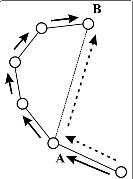
Although beaconless planarization is more efficient, it still requires a considerable overhead and may result in the use of longer routing paths (see Figure 1). In this art-icle, we adopt a novel approach to geographic routing in

Figure 1An example of routing paths with planarization

large-scale WSNs. The main idea isto avoid planarization at all, beacon or beaconless. In our proposed routing protocol, packets are routed using the greedy forwarding mode as long as possible. Whenever the packet gets stuck in a local minimum,the packet is routed along the bound-ary of the hole without requiring a planarizationprocess. Instead, the routing along the boundary of the hole will be performed using a simple mechanism relying on the infor-mation included in the packet header. Moreover, the rout-ing decision at each hop is taken distributedly by the current node and its neighbours by means of a simple

forwarder resolution protocol. Even though similar ap-proaches have already been reported in the literature, our proposed resolution protocol does not require that the nodes get to know their transmission ranges. The oper-ation details and a performance evaluoper-ation of the overall solution are given in Sections 3 and 4, respectively.

The main contributions of this article can be summa-rized as follows:

a) A novel geo-routing protocol ARROW. The protocol is based on simple angle and range calculations to be performed by the sensor nodes without requiring at all a local or global

planarization of the network. We also provide a detailed performance evaluation of ARROW for different network sizes and node densities.

b) A novel forwarder resolution protocol that enables sensors to compute a routing decision allowing the selection of the best forwarder in a distributed way, i.e. in a hop-by-hop basis. This protocol uses simple metrics that can be computed from local

information.

c) An analysis of the proposed forwarder resolution under uncertainty. Differently to previous resolution protocols, the forwarder resolution protocol introduced herein does not require the nodes to have a perfect knowledge of their transmission ranges. Numerical results obtained via analysis and simulation show the effectiveness of the proposed protocol in routing the packets through the network even in the case where the nodes do not have perfect knowledge of their coverage ranges.

The remainder of the article is organized as follows. In Section 2, we describe the most common geo-routing ap-proaches and discuss related work. Our proposed routing algorithm and the accompanying forwarder resolution protocol are explained in Section 3. The protocol perform-ance is evaluated by simulations in Section 4. Section 5 discusses propagation issues and provides some conclu-sions. Finally, in Appendices 1 and 2, we explain the de-tails of the routing metrics and provide a mathematical analysis of the forwarder resolution protocol.

2. Related work

Geographic routing protocols for WSNs are a broad topic in the open literature with a large number of solutions proposed to date. Greedy routing, the most straightfor-ward concept described in the previous section, is very ef-fective, but only in dense networks. When the node density is not high enough, less than eight neighbours in average, there is a high probability that a packet may get stuck in a network local minimum, i.e. in a node that has no neighbours closer to the sink [7]. Many authors simply state that an extra procedure is needed [8,9] while others suggest the use of a flooding mechanism [10] which is time and energy consuming. Face routing which is the most promising recovery solution consists on routing the packet along the hole boundary [11]. This procedure can be further refined in multiple ways, for instance to minimize the routing cost, and is usually combined with greedy routing [7,12-14].

Face routing combined with greedy routing guarantees packet delivery if certain additional conditions are met [15]. However, face routing requires carrying out a previ-ous network planarization process. There are different suitable planar graph constructions like the Gabriel graph or the relative neighbourhood graph [16]. How-ever, this process needs information about the complete neighbourhood of a node in the worst case. Hence, planarization requires that nodes obtain full knowledge of their neighbourhood by exchanging beacon packets [7]. This may be an intensive signalling and maintenance procedure in terms of energy consumption and commu-nication overhead, especially if the topology of the net-work changes frequently.

The alternative approach of beaconless planarization tries to construct a local planar subgraph using as few messages as possible. Recently, a beaconless planarization and forwarding procedure based on a Select-and-Protest

philosophy has been proposed [16] and later extended in [17]. The graph planarization is performedon the run dur-ing data transmission by the Angular Relaydur-ing algorithm: nodes listen to the transmissions in their vicinity and send protests if they become aware that the selection of a potential forwarder may result in intersecting links, according to the Gabriel graph construction [18]. A protesting node becomes the candidate, but the new po-tential forwarder is also a subject to further protests. The process of removing links is continued until there are no more protesting nodes. The selection of the forwarder is based on the least angular distance to the previous hop.

purposes is unrealistic in wireless networks. This is also the case of the mechanism described in [19], where the message delivery is guaranteed without prior planarization provided that the nodes have a perfect knowledge of their radio transmission range.

The mechanism proposed herein is also based on an angular metric, but as we will show in Section 3, it does not require the implementation of a local planarization procedure and still guarantees the delivery of the data packets. In Section 4, we compare the performance of the face routing variant with our proposal and show that the routing cost is significantly reduced. In our routing protocol, the nodes are not required to keep track of the links having been switched off. Moreover, the forwarder resolution protocol, also proposed in this article, is quite effective in identifying from the very first control exchange the best forwarder candidates among the neighbouring nodes. This latter feature allows that a large majority of the neighbouring nodes be released of further control ex-changes which translates on significant energy savings.

A different solution that should also be mentioned is the BoundHole algorithm [20]. As local minima occur at the boundaries of holes, i.e. the regions in the network where greedy routing can fail, BoundHole finds these boundaries in advance, and then routes a data packet along a boundary. BoundHole requires nodes to gather information about their 1-hop neighbourhood enabling them to identify stuck nodes as a previous step to detect a hole boundary. However, routing along the boundary can fail if the destination is inside the hole. In that case, arestricted floodingprocedure is initiated by the bound-ary nodes until a path is found [20]. In either case, the mechanism to be implemented introduces a considerable overhead. Our approach is similar to BoundHole, as we also use the least angle distance to select the next for-warder. However, unlike BoundHole, ARROW does not require to implement the restricted flooding procedure, even if the destination is inside the hole.

Beaconless planarization relies on the assumption that nodes know their neighbours on demand. So there should also be an additional transmission scheme that enables to efficiently forward a data packet from a node to the chosen neighbour, without wasting time and en-ergy in topology discovery procedures. Angular Relaying [16] clearly needs a deterministic procedure but it does not specify how to solve collisions among potential for-warders or protests. Several papers dealing with such schemes and suitable for geographic routing in WSNs have already been proposed. Zorzi and Rao [21,22] intro-duced a scheme to select a forwarder based on the dis-tance that a data packet could progress: a backlogged node sends a packet with its own position when the channel is idle. Each neighbour node then calculates the fitness of the forwarder and responds to the initial

packet using as a basis a time slotted scheme. In the first slot, the best possible forwarders respond and, later, the worse does. Nodes that hear a previous response with-draw their own transmissions. If the initial transmitter receives a single response, it replies with the data packet and the forwarding procedure is successfully finished. If a collision occurs, i.e. two or more neighbour nodes re-spond in the same timeslot, the initial transmitter indi-cates that fact and the colliders reply again with a probability of 50%. This procedure enables to choose the final forwarder in one or few more extra steps.

A similar solution is described in [23,24] and developed in [25]. To decrease the number of exchanged overhead packets, it is proposed to omit the confirmation packets. After a delay period, the nodes under consideration re-spond with the same data packet, forwarding it at the same time and shortening the whole procedure. As the nodes that are competing to forward the packet can have different group of neighbours, the entire scheme can lead to packet multiplication and, as a result, additional energy waste and packet collisions. This problem was later solved in [26] by limiting the area where the potential forwarder can be located and storing the hop number in the packet header.

Both described communication schemes share two shortcomings. First, they do not consider the situation when there are no neighbours closer to the sink than the transmitting node, i.e. the packet is stuck in a local mini-mum. Second, when a collision happens, the forwarder is chosen randomly among the competitors, so it is not guaranteed that the most appropriate neighbour will be selected. The forwarder resolution protocol proposed in Section 3.3 has a similar operation: nodes select a slot according to how good forwarders they are. Our pro-posal, however, does not suffer from these flaws, as after a collision it organizes another competition in order to elect the best forwarder. Some similar ideas can be found in [17], but without any performance analysis.

Finally, it should be noted that these solutions com-bine routing with some MAC functions, but others need an additional specific MAC layer. Interestingly, our pro-posal may be implemented on top of a MAC service that allows nodes to establish activity-sleep periods without knowing their neighbours, like for instance B-MAC [27].

3. ARROW protocol

azimuth state guarantees that the transmitted packet reaches a node closer to the sink than the local mini-mum. Then, thegreedystate is resumed.

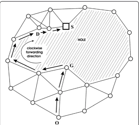
One of the main features of ARROW is to avoid planarization, beacon or beaconless, even in the presence of a hole in the network. Therefore, we use the greedy scheme as long as possible. If the packet gets stuck in a local minimum, it is routed along the boundary of the hole until it reaches a node located closer to the sink than the local minimum (Figure 2). Each routing decision is made with very limited information consisting of the position of the current node, sink node and two previous hop nodes, theleast distanceto the sink and theforwarding direction

(described later). Moreover, each routing decision is taken

distributedlyby the forwarding node using the aforemen-tioned information imbedded into the packet header and actually implemented by means of theforwarder resolution protocolalso proposed in this article.

The flow chart of ARROW is illustrated in Figure 3, while a thorough description and the rationale behind the routing protocol is presented in Section 3.1. A dis-cussion on the processing tasks to be made by the nodes is provided in Section 3.2. Finally, the forwarder reso-lution protocol that allows ARROW to apply the rules in a distributed manner is explained in Section 3.3.

3.1. Routing algorithm

Our routing proposal has been developed with the fol-lowing assumptions:

a) The connectivity between sensor nodes is

characterized by the unit disk graph model [28]. All nodes have the same transmission power and equal circular range. Under these assumptions, the entire network topology can be scaled up or down (dividing all the distances by the nodes transmission range) to set-up the transmission range equal to 1, independently of the transmission power and path loss. In the final section of the article, we discuss the impact of the connectivity model and the

propagation scenarios on the routing protocol performance.

b) The network is connected. A path between each sensor node and at least one sink exists. If there exists more than a sink in the network, the sensor nodes must be aware of the existence of the nearest sinkthey are connected to, not simply the closest one. This assumption ensures that a data packet will not circulate indefinitely around the closest sink to the origin node for which no path may exist.

Figure 3 illustrates the general operation of ARROW. As shown in the figure, ARROW switches back and forth between two states: greedy and azimuth. When a node gets ready to transmit a packet, it initiates the routing process in the greedy state. While in this state, the source node as well as all the nodes in the path to-wards the destination will choose among the neighbours the node meeting the following two conditions: (1) the neighbour with the shortest distance to the closest reachable destination and (2) the neighbour whose dis-tance to the closest reachable destination is shorter than the distance of the current node, i.e. the one currently looking for a suitable neighbour [15]. If such neighbour exists, the node will forward the packet to it. The rout-ing process will proceed in this way until the packet is delivered to the destination or arrives at a stuck node, i.e. a node located at the boundary of a hole (node G in Figure 2) [20]. In this latter case, the current node will be unable to find a neighbour fulfilling the aforemen-tioned two conditions. In order to be able to proceed, ARROW switches to theazimuthstate.

Upon entering the azimuth state, and in order to be able to evaluate the progress of the routing strategy, the distance between the stuck node,G, and the destination,

S, is first stored in the packet header. We will refer to this value as the shortest distanceand it will be denoted by |GS|. While in the azimuth state, the main goal of ARROW will consist of routing the packet around the hole boundary, searching for a path towards the destin-ation. ARROW will switch back to the greedy state as soon as a node closer to the sink than the stuck node is reached. Furthermore, and in order to be able to prop-erly operate under all conditions, while in the azimuth

Figure 2ARROW protocol: a message originated inOis

transported according to greedy state toG(local minimum).

state, ARROW will register the coordinates of the two previously visited nodes in the packet header, (x1,y1) and

(x2,y2), where (x1,y1) refers to the very last visited node.

Initially, (x1,y1) is set equal to the coordinates of S, i.e.

the stuck node, and (x2,y2) is not set.

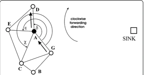
Upon entering the azimuth state and once having updated the header data, ARROW starts by deciding the way to take to surround the hole. ARROW chooses as next node, from now on referred as the forwarder, the neighbour of the stuck node, G, with the smallest azi-muth angle relative to the direction to the sink (see Figure 4). The choice of the first forwarder determines the forwarding direction around the hole, i.e. clockwise or counter-clockwise. In this way, ARROW will attempt to surround the hole following the forwarding direction

as long as it finds a suitable forwarder. ARROW then proceeds by choosing the node with the smallest angle relative to the direction of the edge of the previously vis-ited edge as the next forwarder (Figure 5). The angles

are calculated taking into account the forwarding direc-tion being followed. This is to say, if ARROW has de-cided to surround the hole clockwise, the angles are calculated in the counter-clockwise direction and vice versa (Figure 5). In the worst case, if the current node has no further neighbours other than the previous neighbour, the packet will have to be sent one-hop back. Then, the forwarding process resumes following the same for-warding direction, i.e. the node with the smallest angle relative to the direction of the previously visited edge will be chosen as the next forwarder.

This simple 2-state procedure guarantees the delivery of packets in planar networks. To verify the correct op-eration of ARROW under these conditions, simply con-sider the stuck nodeGand the circle centred at the sink

Swith radius|GS|.In this case, ARROW will not return to the greedy state as long as it has not reached a node closer to the sink than the previous local minimum. Once in the greedy state, the packet may reach the sink

or another stuck node,U. Since |US| < |GS| and because the network is composed of a finite number of nodes, by switching back and forth between thegreedyandazimuth

states, ARROW guarantees the delivery of the packet to the final destination. A rigorous demonstration of the prin-ciples on which the ARROW protocol has been developed can be found in ([15]: Theorem 4, [20]: Lemma 3.13).

In the case of a non-planar network, further provisions have to be put in place in order to ensure the delivery of the packet to its final destination. In a non-planar net-work, the existence of intersecting edges lead to routing loops (Figure 6b). In order to overcome this problem, a graph planarization procedure could be performed. However, such procedure requires the exchange of mes-sages which implies the definition of a protocol for this purpose [16] and the handling of data structures to be stored in the forwarding nodes. In this article, we

propose a simple and efficient solution whose only re-quirement consists of registering the coordinates of the last two visited nodes in the packet header. While in the

azimuth state and in order to properly follow the hole boundary, each node will have to verify that the edge to be used is not intersecting the already visited ones and that there is in fact a hidden edge leading to a better po-sitioned node.

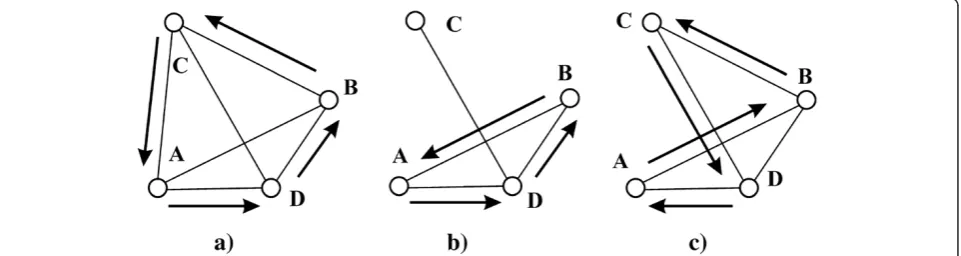
Our proposed mechanism is built on the results reported in [29]. In that study, the authors have shown that if two links AB and CD intersect in a unit disk graph, only three possible cases may arise, as shown in Figure 7. Case (a) causes no problems: while operating in the azimuthstate, ARROW will traverse the exterior boundary (links BC, CA, AD and DB), visiting in the worst case the four nodes. Hence, a better positioned node will always be reached. However, the other cases may cause a packet to fall into a loop. In case (b), if the packet arrives to nodeA,BorD, it will not be forwarded to nodeC. It could use the linkCDto reach it, but the azi-muthstate rules do not allow for that. On the other hand, in case (c), all the nodes can be reached, but the routing al-gorithm is unable to follow the hole border, because it is unaware of crossing a link having been previously visited. See also Figure 8, where this case is explained with further detail. Hence, to avoid loops and errors in cases (b) and (c), we derive a simple stepwise procedure.

In order to be able to identify crossing edges, the mechanisms proposed herein require to make us of the nodes coordinates of the two previously visited nodes be recorded in the packet header previously described. The proposed mechanism can be simply stated as below.

First, backward rule: the current node additionally broadcasts the coordinates of the two last hop nodes. Then, each neighbour node locally determines the rela-tive positions of the links and decides if it can serve as a potential forwarder. If the link from the current node to the neighbour crosses the penultimate edge, the neigh-bour does not propose itself and remains silent. An ex-ample is given in Figure 8, where the node B does not propose itself as a next hop for the node A, as linksAB

and CDare intersected. The details on how the relative positions are obtained by the nodes are described in Section 3.2. The final routing decision is made by the current node after receiving the responses from all po-tential forwarders. Let us note that this procedure obtains the same results as the procedure of avoiding nodes in the

forbidden region, defined in [20], which ensures that we are correctly following the hole boundary. The backward rule solves the problems of case (c) from Figure 7, inde-pendently of the node where the packet arrives.

Second, IC triangle rule: the case (b) from Figure 7 shows that it is possible for the routing protocol to miss the only path to the sink. The path could be not accessible

Figure 4An illustration of the first hop in the azimuth state (a part of the network topology is shown).The packet has just reached nodeGwhich is a local minimum. The next hop node is chosen among all the neighbours of the nodeG, comparing their azimuth angles relative to the direction to the sink. As_α<β<χ,the nodeAwill be the next hop. It also determines the forwarding direction: clockwise around the hole.

Figure 5Next step of the azimuth state (continuation after

from the boundary of the hole because of the crossing edges (Figure 6b) and thus, a transmitted packet may fall into a routing loop.

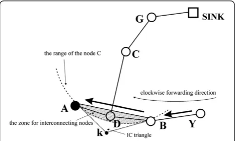
Our solution is depicted in Figure 9. At each hop, e.g. fromBtoA, it should be verified if there is a link between a certain node located farther from the hole boundary (let us call itD) to a node located closer to the sink and non-reachable neither fromAnor fromB(let us call itC). In order to avoid rooting loops, we have to find if such a nodeDexists and forward the packet to it. If it exists, it must be located within the interconnecting (IC) triangle

having as verticesA,Band the pointk(Figure 9). The IC triangle is isosceles with the linkABbeing its base and the angles∠ABkand∠BAkbeing equal to 30° and∠AkBequal to 120°. In other words, a search within the IC triangle en-sures that the nodeDinterconnecting toCwill be found, as proved below.

Theorem: The interconnecting node D, if exists, is al-ways located in the IC triangle as defined above.

Proof:We are looking for nodeDconnected with node

C, this latter fulfils the following two conditions: (1) it is located out of the range of both A and B and (2) it is closer than both A and B to the closest reachable sink. Thus, according to the unit disk graph model, the dis-tance DC must be shorter than AC and BC. If node D

exists, it must be located on the opposite side of the link

AB to C: if not, D would have been found before as a next hop node instead ofA. Thus,Dmust be located in the circle centred at Cand with the radius equal to the radio transmission range, while at the same time the links AB and DC must cross. Consequently, the area where D can be located is limited to the shaded area shown in Figure 9. The size of this area increases as the distance between A and B increases. The size is max-imum when A and B are located just on the transmis-sion radius of C. In the borderline case, A, B and C

create an equilateral triangle, where A and B are interconnected with each other, but not with D. In this

Figure 6A planar network (a) and non-planar one with intersecting links (b).A packet is trying to reach the sink while inazimuthstate, from the nodeY. The first hop is the nodeB. Then, keeping the clockwiseforwarding direction, the next hops are chosen. In the planar network, the packet eventually reaches the sink. In the non-planar one, the packet from the nodeBwill be forwarded toA, because∟YBA<∟YBD<∟YBE <∟YBXand the nodeD, being the only way to the sink, does not lie on the hole border. Note, that theforwarding directionwhich is clockwise around the hole means the counter-clockwise calculation of the azimuth angles (see also Figure 5) and the counter-clockwise circulation around a part of the network. As a result, the packet will remain circulating in a loop.

Figure 7Three only possible cases of two crossed linksABandCD.Let us assume that the sink is located above the considered nodes

case, the circle determined by the transmission range of

C is tangent to the edges Ak and Bk, while the whole shaded zone is located inside the IC triangle. Hence, in all the cases the interconnecting node is located inside the IC triangle.■

Checking the IC triangle, the nodeDcan verify if it is a potential interconnecting node even if the radio trans-mission range is unknown. The node D only needs to examine if the angle∟ADBis larger than 120°. This is a simple procedure that can be done by calculating the cosine function of the angle ∟ADB, as explained in Section 3.2.

To summarize, ARROW withIC triangle ruleproceeds as follows. After a hop in theazimuthstate, it looks for a

potential forwarder in the IC triangle. If such node exists (e.g. the nodeDin Figure 9), the packet is forwarded to it. If there are two or more such nodes (e.g. D1 and D2 in

Figure 10), the protocol chooses the nodeDiwith the lar-gest angle ∟ADiB (closest to link BA). Then, this node sends a request looking for a node located on the opposite side of (above) the link BA (the node C in Figure 9). If eventually nodeCexists, it is chosen as a forwarder. Note that after forwarding the packet toC, the appropriate node

DiandB(notA) are registered as the two last hop nodes having been visited in the packet header, in order to follow properly the border of the hole.

In the very unlikely situations when there is more than one such a node (see the nodesC1andC2in Figure 10),

we choose the nodeCjwith smallest angle∟CjDiB. If the nodeDhas no appropriate neighbours, the protocol seeks anotherDinode in the IC triangle and the procedure is re-peated. If there are no more Di nodes, the packet is forwarded back to the nodeAand the data transmission is resumed along the borderline of the network.

In order to perform all the procedures, each node only needs to check the relative angles, which are calculated on the basis of its own position and the two last-hop co-ordinates. Therefore, the following information is needed and broadcast by the current forwarder when looking for a next forwarder:

(a) the coordinates of the current forwarder, (b)the coordinates of the two last hop nodes, (c) theforwarding directionand

(d)theleast distancefield.

In the greedy state, the situation is even simpler, as the coordinates of the current forwarder are sufficient

Figure 8The azimuth state, clockwise forwarding direction.As

δ<ε, the next hop after the nodeAwould be the nodeB. The backward ruleprevents such a situation: the candidates for potential forwarders (nodesBandE) check if their links with the current node (linksABandAE) are not intersecting the penultimate hop edge (the linkCD). Because ofABandCDintersection, the nodeBis not considered as a potential forwarder and, eventually, the packet is routed to the nodeE.

Figure 9The interconnecting nodes can be located only in the

indicated shaded zone.For the sake of simplicity of the calculations performed by nodes, the zone is extended into the so-called IC triangle.

Figure 10The case of multiple nodes located in the IC triangle

and the remaining data do not need to be broadcasted. It is worth mentioning that the whole above procedure is donedistributedly and without any additional infor-mation about the neighbourhood. That is, when a node announces to all its neighbours that it has a packet to forward, each neighbour can locally and independently from all the other neighbours evaluate its fitness as the best forwarder. On this basis, the neighbours decide if they are suitable candidates to the best forwarder and if so they reply to the announcement issued by the current node. In order to actually come out with the best for-warder, the node and its neighbours implement the for-warder resolution procedure described in Section 3.3. One of the main goals of this protocol is to coordinate the exchange of control packets among the current node and its neighbours.

There are also significant advantages of the proposed solution compared with other beaconless approaches based on local planarization. First, the nodes do not need to listen to all the radio transmissions in their vicinity in order to remove the non-planar links: if a node is not suitable as a forwarder, it can go into idle state and save energy. Second, we can avoid forcing the nodes to re-member (store) which radio links are switched off. Finally, local planarization requires checking all the pos-sible local forwarders in a suitable planar graph, usually a Gabriel graph. The IC triangle area is around 37% of the area of the Gabriel semicircle, so the number of situa-tions and nodes involved when we need to proceed with the procedure described above is smaller than in local planarization. Furthermore, differently to other routing protocols that do not use planarization [16], ARROW does not require that the nodes get to know their radio ranges in order to successfully route the packet through the network. It should be also stressed that the proposed solution introduces only a minimal overhead associated withRequest-To-Send(RTS) packets (typical for wireless routing) and very short (few bytes)Clear-To-Send(CTS) packets of the forwarder resolution protocol, as explained in Section 3.3.

3.2. Local calculations

All the routing decisions are made after the analysis of the relative positions of the current node, the nearest sink and two previous hops. The required computations are very basic and not too demanding for sensor proces-sors. In particular, as it was explained in the previous section, the nodes should be able to:

a) compare relative angles,

b) calculate the cosine function of an angle (when checking an IC triangle),

c) check if two links cross (to avoid routing loops and errors in theazimuthstate).

(a) To compare the relative angles, we propose that each potential forwarder node calculates the following expression:

coordinates of the potential forwarderF, the sinkS and the transmitting nodeO, respectively. The rationale behind (1) is as follows. According to the well-known definition of the dot product, we can calculate the cosine function of the angle∠FOS:

cos∠FOS¼

Note that∠FOSis the azimuth angle of the potential forwarder relative to the direction to the sink. The square root in (3) equals the distance from the sink to the transmitting node and is constant in the metrics of all potential forwarders. Thus, the neighbour node with the largest metricahas the least azimuth angle.

(b)Calculating the cosine function is the simplest method to verify if a node is located inside an IC triangle. Using the notation from Figure9, the node Dshould check if cos∠ADB<–0.5. Recalling again

the dot product definition,Dshould verify that:

xAxD

(c) In order to check if two vectorsAB andCDare crossed, we can calculate if pointsAandBare on the opposite sides of the line given by pointsCand D.To meet this condition, we check the angles

xAxC

ð ÞðyDyCÞ ðxDxCÞðyAyCÞ

½

½ðxBxCÞðyDyCÞ ðxDxCÞðyByCÞ

<0 ð5Þ

At the same time, pointsCandDmust be on the oppos-ite sides of lineAB: a condition analogous to Equation (5) must also be met. Only if both conditions hold, the links cross and, thus, the backward rule applies.

3.3. Forwarder resolution protocol

The forwarder resolution protocol described herein has been designed to operate together with ARROW. It is similar to that presented by Zorzi and Rao [21,22], but more general: it works also if a transmitting node has not any neighbours closer to the sink. It follows the idea of splitting the set of potential forwarders into smaller sets until the correct one is chosen, so it guarantees selecting the best neighbour. It does not need any infor-mation about the relative neighbourhood prior to send-ing a data packet.

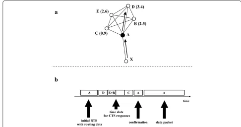
The procedure starts when a node has a packet to for-ward, or is the source of a message. After checking if the channel is idle, it sends an RTS packet, which consists of the routing data and indicates that the node is looking for forwarders. After the initial RTS, time becomes slot-ted and a frame of timeslots follows (see Figure 11). All the neighbours compute theirrouting metrics, described in Appendix 1, to decide if they are potential forwarders.

The metrics are mapped into the length of the frame,N

(e.g. if N= 4, the routing metrics will provide an integer in the interval [1..4]). The potential forwarders select a timeslot to reply with a CTS short packet, according to the computed metric: first slot if metric is 1, second one if it is 2 and so on.

For the RTS sender, only the first slot with a single re-sponse is relevant: that node is the next forwarder. Then, it sends a short confirmation packet, so as to let non-involved nodes go to sleep. Immediately after that the data packet is sent (see Figure 11).

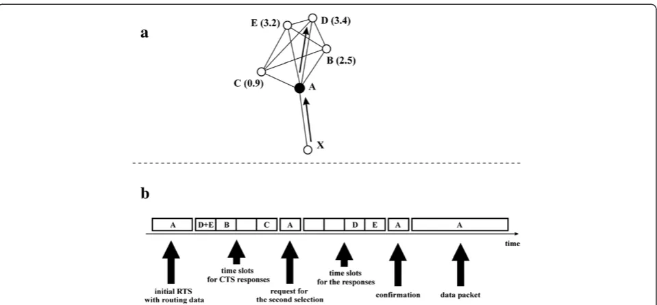
However, it is possible that two potential forwarders compute similar metrics and they both respond in the first occupied slot, resulting in a collision. Then, the RTS sender cannot decode their responses. Thus, it sends another (though very short) RTS showing only the index of the collided slot, followed again by a frame ofN

slots (see Figure 12). But in this case, only the nodes having collided previously are allowed to reply. The re-sponses (CTS) of the competing nodes are remapped into theNslots again, proportionally to their metrics. As their range is now smaller (from N–1 to N only), it is very likely that they select different slots. In the worst case, if there is another collision, this process is repeated until the first occurrence of a slot with a single reply.

Note that all collisions or replies following a slot with a single reply are ignored. The details on the mechanism used for the allocation of the timeslots in both routing states, i.e. the mapping of routing metrics, are given in Appendix 1.

Figure 11The forwarder resolution protocol. athe network topology—the node metrics are given in brackets.bthe consecutive

Let us also remark that all the timeslots and packets, except the RTS with initial routing data and the data packet, are very short. Just a few bytes are enough to let other nodes know that the channel is occupied or to in-form that a collision has happened, as even the ad-dresses of nodes are not needed.

Finally, in all the cases, only one neighbour is chosen as a forwarder. The entire forwarding procedure requires sending the initial routing data and reserving at least

N+ 1 short timeslots (Nslots within the time frame for neighbour responses and 1 slot for the final confirmation sent by the initial node). In the case that a collision oc-curs or if the routing state changes, another selection round is initiated, i.e. other N+ 1 short timeslots are generated in order to put the nodes replies there. From this description, it is clear that the overhead introduced by the ARROW routing protocol and the described for-warder resolution protocol is limited to the initial RTS packet with routing data and the short CTS/confirm-ation packets. The data packet is sent afterthe proced-ure has been able to choose the best neighbour. The nodes not having been chosen as the forwarder can go to sleep immediately after realizing that the node offer-ing the best guarantees has been picked up.

An important design parameter is the length of the frame,N. In order to reduce the complexity of the scheme, the best is to assign a constant value toN. Clearly, a small

N allows to get the neighbour responses quickly, but it also increases the probability of a collision. In Appendix 2, we present an analysis proving that, depending on the net-work density, the forwarding procedure is optimized for

N= 2 or N= 3. The mathematical analysis has been

restricted to the case when the protocol operates in the

greedy state. The general performance for the whole ARROW protocol in both routing states is evaluated with the aid of computer simulations in the following section.

4. Protocol performance results

In order to validate ARROW, we performed extensive C++ computer Monte-Carlo simulations for a wide spectrum of working parameters: network size, node density, number of sink nodes, error of the transmission range and number of timeslots in the time frame. To characterize the connectivity between sensor nodes, we used the well-known unit disk graph model. However, as the transmission range is not known by the nodes in real wireless networks, we assumed that the real range d

could be different to the range d'used by the nodes to calculate the routing metrics (see also Appendix 1). We called ratiod'/dthetransmission range error.

The sensor network topology was generated randomly, with a two-dimensional uniform distribution of the nodes and the sinks in a square field. Basically, three cases of sensor networks were investigated: (a) a network with 1,000 nodes and 10 sinks, (b) 1,000 nodes and 50 sinks and (c) a large network with 10000 nodes and 100 sinks. These cases were considered to study the influ-ence of network size and percentage of the sinks on the protocol performance. In order to obtain different net-work densities, the whole area with the nodes was scaled accordingly, i.e. its dimensions were increased or de-creased, keeping the same number of sensors. For low-density networks, a large number of the nodes were not connected, i.e. there was no path between them and any

Figure 12The forwarder resolution protocol when a collision forces the initial node_Ato send a request for the second selection of

sink. In all scenarios, we simulated the full network, counted the number of not connected nodes and then, we calculated the simulation results only for the connected ones. All the simulations were repeated at least 5,000 times, thus all the 95% confidence intervals were smaller than 3% of the measured values.

In Figure 13, the percentage of connected nodes is shown. For a given network density, the connectivity de-pends on the percentage of the sinks rather than the net-work size. For all the cases, a low netnet-work density (below four nodes per unit disk area) is rather not ad-vantageous, as the majority of the nodes is isolated and has no connection to any of the sinks. The most favourable networks in terms of cost have densities be-tween 5 and 8 nodes per unit disk area (depending on the sinks/nodes ratio). This is a reasonable trade-off be-tween having the majority of the nodes connected and not wasting the resources for redundant nodes. In numerous papers, more dense topologies are considered [23,24,30], also as a solution to keep the network connected when some nodes deplete all their energy. However, bearing in mind the low-cost criterion followed in most WSN de-ployments, increasing the number of nodes may substan-tially increase the costs of deployment and maintenance rather than enhance the operation of the batteries. How-ever, the best network configuration will very much de-pend on the nature of the end application.

The routing costs of ARROW and Angular Relaying [16] protocols are compared in Figure 14. The cost of routing is defined as the average number of hops done with the protocol to reach the sink divided by the aver-age number of hops in the shortest possible path [7]. This cost not only gives an idea of the energy spent for

the subsequent retransmission of a packet, but also of its end-to-end delay. It also informs about the approximate overhead of ARROW, as in each hop we have exactly one RTS and at least one CTS packet. The actual num-ber of time slots with CTS packets depends not only on the network density, but also on the frame size and the ratio between the real and estimated radio transmission range (see Figures 15 and 16). The routing cost is the largest in case of the mid-density networks: here, the greedy routing has a significant probability to fail and the azimuth state is required very frequently. In low-density networks, the topologies are very simple, with many nodes not-connected (see Figure 13). On the other hand, when the density is high, there is a large probabil-ity that the whole routing path can be done in thegreedy

state. A higher percentage of sinks (see the scenario with 50 sinks) also decreases the routing cost substantially. Obviously, the average routing paths are also shorter, in this case, and it results in larger energy savings.

In all the scenarios, ARROW exhibits similar routing cost than Angular Relaying, except in the case when the mid levels of network density. Under these latter scenarios, ARROW shows its value outperforming the Angular Relay-ing protocol. These results clearly show that ARROW is able to route the packets in a very effective manner, i.e. via a shorter path than the ones used by Angular Relaying. Therefore, it effectively reduces the number of unnecessary hops introduced by the planarization process. Unlike An-gular Relaying, it is achieved without forcing the nodes to remember which radio links should be switched off. In addition, we reduce the number of listening nodes in each transmission: part of the sensors can go into a sleeping state just after becoming aware that they are not proper

forwarders. In the Angular Relaying algorithm, the nodes need to listen longer in order to check the links planarity.

Comparing ARROW with other geo-routing algo-rithms like Angular Relaying, it would be also interesting to verify the real memory usage and energy consump-tion. This, though, depends strictly on the specific hard-ware where the geo-routing protocol is implemented and thus it is a topic for future work.

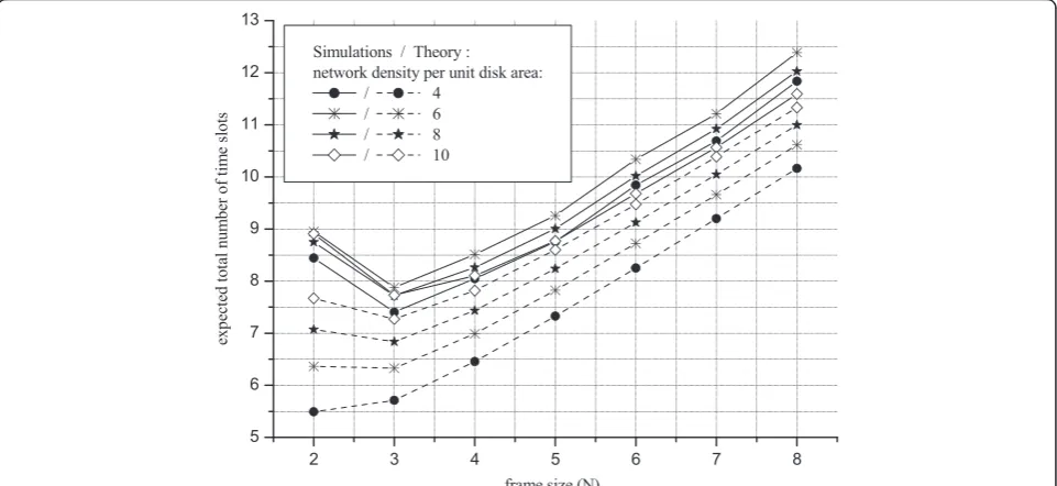
We also investigated the performance of the forwarder resolution protocol, described in Section 3.3, as a func-tion of the frame sizeN. The procedure of forwarding a single data packet requires reservingN+ 1 timeslots and, in the case of a collision, other N+ 1 timeslots, and so on. Thus, we studied the expected total number of timeslotsEsrequired for a single routing hop, what gave us a measure of the protocol overhead.

Figure 14The algorithm cost for ARROW and Select-and-Protest protocols.It also informs about the number of RTS packets, as there is

exactly one RTS packet per hop.

In Figure 15, the results for the network consisting of 1 000 nodes and 10 sinks are presented. The minimal Es occurs forN= 3: no more than 8 slots are required to per-form the forwarding procedure, it means 2 time frames, with 3 slots each one, and 2 confirmations (see Figure 12), in average. As a comparison, the theoretical results (only the greedy state, see Appendix 2) are given. Simulations show larger Es values than theoretical calculations, par-ticularly for the density of 4 or 6 nodes per unit disk area. It is understandable, as theazimuthstate is more frequent there. This routing state is usually less efficient in limiting the number of timeslots (see Appendix 1).

In these simulations, we assumed that all the nodes knew their maximum transmission ranged. Since this parameter is not known for the nodes in real networks, we tested two additional scenarios: when the assumed transmission range

d'is lower or higher than the real ranged. As explained in Appendix 1, our protocol can manage that issue; however we are expecting that the timeslots are not used effectively. Ifd0<d, the first timeslot is overloaded, while ford0>dtoo many CTS responses occur in the last slot. Both situations can lead to CTS collisions and, in consequence, they could increase the overhead of the resolution protocol, though, as presented in Figure 16, the proposed protocol is rather robust against the errors in the transmission range. For the suggested case of N= 3, even ifd0=d/10,Es does not in-crease by more than six additional slots compared to the ideal case of the known transmission range.

5. Conclusions

Numerous current and envisioned applications, e.g. envir-onmental, agricultural, military or research ones, require

large-scale WSNs. In contrast with small-scale WSNs, the objectives like the low node cost, scalability and robust-ness against irregular and changing topologies are crucial for the good performance and profitability of a network with a huge number of nodes. The design of the WSN communication protocol for a large-scale network should strictly concentrate on fulfilling these goals.

It is the localization ability which enables to achieve the abovementioned design objectives. If a sensor node knows its own position and the position of the nearest sink, it can just send a data packet in the proper direc-tion, avoiding the maintenance of routing tables. The location-based transmission protocols are more scalable and resilient to adverse network topologies. Also, they effectively limit the protocol overhead, simplifying the communication and decreasing the energy consumption. In this article, we propose and discuss ARROW: a new geo-routing protocol for WSNs. ARROW avoids local planarization, while simultaneously guaranteeing mes-sage delivery in non-planar networks without requiring sensors to keep any topological data in their memories. ARROW is based on distance and angular metrics ap-plied together with simple rules in order to avoid routing loops because of crossing links. We also present a for-warder resolution protocol integrated with ARROW that enables each sensor to efficiently and distributedly choose the best neighbour in the forwarding process according to the ARROW rules. The nodes do not need to be aware of their neighbours, making the communica-tion more robust against network topology variacommunica-tions. Each node decides if it is a potential forwarder by com-puting a simple metric only with knowledge about its

own position, current forwarder and two previous hop positions. These metrics are also used to distributedly select the next forwarder.

Our extensive simulation results validate both pro-posed protocols. They show that ARROW effectively re-duces the number of hops comparing to beaconless planarization techniques. The protocol overhead could be very limited, especially when the transmission frame size is chosen carefully. Moreover, the protocols are very scalable in sensor networks of different size, density and percentage of sink nodes. Finally, although the forwarder resolution protocol operates optimally when the trans-mission range is known, it also shows a good robustness when this parameter is not known for the sensors.

ARROW has been designed to exploit geometric prop-erties of the unit disk communication model. Neverthe-less, the assumed unit disk graph model is only a rough approximation of the network connectivity. In real net-works, a wireless channel fading may result in a network topology where the proper routing path is contrary to the geographic intuition that stands behind the idea of geo-routing. In such a scenario, the message delivery can be guaranteed only with very extensive and energy-consuming topology discovery procedures. While more research is re-quired on this topic, a good connectivity model suitable for routing simulations in wireless networks is also an open issue. There are numerous proposals that are able to neatly characterize the propagation channel between two wireless devices. However, we still need a decent model of spatial correlations of wireless communication channels which are crucial for the performance of routing protocols.

Appendix 1: Routing metrics

To clarify how the neighbour nodes choose proper timeslots, we consider both routing states separately. In the greedy state, only the nodes that are closer to the sink are competing. The length of the frame is N. As-suming that the maximum transmission range d is known to all the sensors, after the transmitting nodes send initial routing data, each neighbour can calculate its metric with the following formula:

mi¼N:

L0Li

d ð6Þ

where L0 and Li are the distances to the sink from the transmitting node andith neighbour, respectively. Now, for the timeslots indexed as N−1, N−2, . . ., 1, 0, the mapping to the slot number is calculated as the floor function of its metric. If a collision occurs in the first oc-cupied slot, the selection procedure needs to be re-peated. However, the selection is now limited only to the nodes that have sent the colliding packets, as we know that the best forwarder is among them. If the collision has a place in the slot with the index M (the previous

slots, if any, were not occupied), the nodes that have responded in that slot are recalculating their metric:

mi2¼N:ðmiMÞ ð7Þ

and they are responding in the timeslot with the index being the floor function of their new metrics mi2. This procedure is repeated until there is only one response in the first occupied slot.

In a real case, range d is not known to the wireless nodes. Instead, the nodes must use a certain value d'

possibly close to the real range. The theoretical range can be derived from the appropriate propagation models for WSN [6]. There are two cases: if d0>d, the protocol works properly, but the timeslots are not used effect-ively: the first slots are occupied rarely. The situation is more difficult if d0<d. Then, it can happen that some nodes have their metrics larger thanN. Of course, such nodes could just respond in the first slot but, if there are two or more of them, the collision cannot be resolved in any number of retrials, as all these nodes have the max-imum value of the metric. Therefore, we propose to proceed as follows. If the collision occurs in any timeslot but the first one, the metrics are recalculated according to (7) and the selection procedure is continued as we de-scribed before. But if there is a collision in the first slot, instead of recalculating the metrics, the nodes that responded in the first slot divide their metrics by 2. If the collision happens in the first slot for the second time, the metrics are again divided by 2, and so on, until we are sure that there is no more than one neighbour node with the metric larger thanN. In Section 4, where the forwarder resolution protocol performance is evalu-ated, we considered several situations when the max-imum transmission range is not known to the nodes and it is under- or over-rated.

In the azimuth state, there are three sub-cases that must be considered. Choosing a forwarding neighbour, the priority should be given to the nodes that are closer to the sink than theleast distancevalue remembered in the data packet (see Section 3.1). If there are no such nodes, the packet must be transmitted to a node in the IC triangle with respect to the previous hop (if this hop was also the azimuthone). Eventually, other neighbours may be potential forwarders, according to their azimuth angle (see Figure 5). Thus, we need multiple metrics, suitable to these three categories. For the nodes closer to the sink than theleast distancevalue, we propose

mi¼N 1 3þ

L0Li

3d : ð8Þ

mi¼N1

4 cosβþ2

3 : ð9Þ

The angle βis equal to the angle ∠BCiAand can be computed from the information broadcast in the RTS packet, as described in Section 3.1. As ∠BCiA∈(120°, 180°), the nodes located in an IC triangle receive metrics∈ (N–1, N–1/3). All the nodes classified into these two categories occupy the first timeslot. Concluding from our experience of computer simulations, a single slot is enough, as most of the neighbour nodes fall into the third cat-egory and their metrics are calculated according to their azimuth angles:

mi¼

N1

ð Þ:cosαþ3

4 ; α≤180

N1

ð Þ:1 cosα

4 ; α>180

:

8 > < >

: ð10Þ

This metric is constructed so that the nodes from the third category are distributed into all the slots but the first one, proportionally to the angle α, that is, their an-gular distance to the current forwarder.

It is worth to remark that, for theazimuthstate, com-peting nodes can be located in the whole unit disk area around the current forwarder. In comparison, for the greedy state, they can occupy only half of the disk area: the nodes farther to the sink do not respond. Thus, we can conclude that, for greedy state, the forwarder reso-lution protocol is more efficient in terms of limiting the number of timeslots. It is confirmed by the simulations, as shown in Figure 15.

Appendix 2: Number of slots in the time frame Here, we present the mathematical analysis to compare the ARROW performance for different time frame sizes. Still, the analysis is valid only for thegreedystate. In the

azimuth state, we cannot assume that the node density is the same in the whole range of a transmitting node, as we know there is aholenearby.

Let us assume that the transmission range of all the nodes is equal to d (according to the unit disk graph model). The nodes in the analysed network are distrib-uted randomly with a two-dimensional uniform distribu-tion over an unlimited area and their density, i.e. the number of nodes per circle with radius dis ρ. Now, let us consider a situation where a node Ais going to for-ward a packet (Figure 17) and it broadcasts the RTS. The closest sink is at the distance L, whereL>d. If the number of timeslots is equal toN, the neighbours of the nodeAare grouped intoNzones, according to their dis-tance to the sink. Thejth zone contains the nodes located in the distance∈(L−d+ (j−1) ·d/N,L−d+j·d/N) from the sink. The nodes respond in timeslots according to the zone numbers: the ones from the first zone (closest to the sink) respond in the first timeslot, etc. The nodes that are farther to the sink than the nodeA, do not respond at all. If a collision happens in the first occupied slot (a collision after a slot with a single reply can be ignored, see Section 3.3), the next selection round (nextN+ 1 slots) is required. In such an adverse situation, the zone where the colliding nodes are located needs to be further divided into Nsmaller sub-zones. Only these nodes will respond again and the forwarder will be selected among them. If a collision occurs once more, the sub-zone with colliding nodes is again divided intoNsmaller sub-zones and next

Figure 17An example of the forwarding process for the time frame with four slots.If for example the area of the second zone needs to

N+ 1 slots are created, etc. The whole procedure is re-peated until there is no collision in the first occupied timeslot. We can calculate the expected total number of timeslots as follows:

Es¼ðNþ1Þ: X1

i¼1

i:Pi; ð11Þ

where Pi is the probability that the best forwarder is chosen in ith selection round. The probability P1can be

expressed as follows:

Equation (12) can also be explained as follows. In order to have the forwarder chosen in the first selection round, there should be exactly one node in the first zoneor no nodes in the first zone, and one node in the second zone

or no nodes in the first two zones, and one node in the third zone, and so on. The scaling factor 1

1p0ðLd;LÞ is the

result of the fact that we are considering only thegreedy

state, so we need to assume that there is at least one node in one of the zones. When i> 1 (a case withi–1 colli-sions), there is at least one zone where there are two or more nodes and there are no nodes in other zones located closer to the sink. The zone with nodes is divided i–1 times, thus, there is no collision in the first occupied timeslot during the final selection round. Accordingly,Pi>1

is equal to

The variableRidescribes how the nodes should be dis-tributed in order to have exactlyi–1 collisions. After all zone divisions, we have Nsub-zones. There are two or more nodes in total in these sub-zones, as we know that we had a collision in the previous selection round. But, there is no collision in the ith selection round, so there is only one node in the first occupied sub-zone and other nodes (at least one) are located further. Equation (13) shows that there are no other nodes located closer.

In all cases, the probabilitypk(r1,r2) is given by a

two-dimensional Poisson distribution with the node densityρ:

pk¼ ρ

:S

ð Þk

k! :e

ρS_{: ð16Þ}

where S is the area of a zone, zone or multiple sub-zones. Its borders are determined by radiir1andr2and it

can be expressed as (see also equations (3–5) in [21] or thecircular segmententry in [31]) follows:

S¼d2arcsinx2

Finally, to obtain Es, we need to compute the infinite sum given in (11). On the basis of numerical calculations, we can state that limiting the number of sum elements to 15 is sufficient, as the next element does not change the result by more than 0.05%.

We compared Es for different values of N, testing three cases:L= 2d,L= 10dandL= 100dfor node dens-ities between 4 and 10. The minimal values of Eswere obtained for

a) N= 2, whenρ≤5 or (ρ= 6 andL= 2d),

b) N= 3, whenρ≥7 or (ρ= 6 andL> 2d).

Therefore, fixing a frame ofN= 3 timeslots is usually a good choice for the scenarios of real interest, as the

greedy routing needs to be supported by the azimuth

Competing interests

The authors declare that they have no competing interests.

Acknowledgements

This study was performed thanks to scientific cooperation efforts taken under the frame of the COST Action IC1004. It was supported by the Spanish MICINN, Consolider Programme, Plan E funds and CALM TEC2010-21405-C02-02,“Programa de Ayudas a Grupos de Exelencia de la Region de Murcia, Fundacion Seneca”programmes. It was also co-funded by European Commission FP7 Programme UNITE and FEDER funds, under Grants CSD2006-00046 and TIN2009-14475-C04-03.

Author details

1

Department of Telecommunications, AGH University of Science and Technology, al. Mickiewicza 30, 30-059, Krakow, Poland.2_{Department of} Information Technologies and Communications, Universidad Politécnica de Cartagena, ETSIT, Campus Muralla de Mar s/n, 30202, Cartagena, Spain. 3

Albacete Research Institute of Informatics, University of Castilla-La Mancha, Campus Universitario s/n, 02071, Albacete, Spain.

Received: 21 October 2011 Accepted: 1 March 2013 Published: 1 April 2013

References

1. H Karl, A Willig,Protocols and Architectures for Wireless Sensor Networks(John Wiley & Sons, Chichester, UK, 2005)

2. I Stojmenovic (ed.),Handbook of Sensor Networks. Algorithms and Architectures(John Wiley & Sons, New Jersey, 2005)

3. N Patwari, JN Ash, S Kyperountas, AO Hero III, RL Moses, NS Correal, Locating the nodes: cooperative localization in wireless sensor networks. IEEE Signal Process. Mag.22, 54–69 (2005)

4. C Wang, L Xiao, Sensor localization under limited measurement capabilities. IEEE Netw.21, 16_–23 (2007)

5. P Kulakowski, J Vales-Alonso, E Egea-Lopez, W Ludwin, J Garcia-Haro, Angle-of-arrival localization based on antenna arrays for wireless sensor networks. Comput Electr Eng36, 1181_–1186 (2010)

6. R Verdone, D Dardari, G Mazzini, A Conti,Wireless Sensor and Actuator Networks–Technologies, Analysis and Design(Academic, London, 2008) 7. F Kuhn, R Wattenhofer, A Zollinger, An algorithmic approach to geographic

routing in ad hoc and sensor networks. IEEE/ACM Trans. Netw.16, 51_–62 (2008)

8. L Blazevic, S Giordano, J-Y Le Boudec, Self-organized terminode routing. Clust. Comput.5, 205_–218 (2002)

9. B Blum, T He, S Son, J Stankovic,IGF: a state-free robust communication protocol for wireless sensor networks, Technical Report CS-2003-11(University of Virginia, USA, 2003)

10. I Stojmenovic, X Lin, Loop-free hybrid single-path/flooding routing algorithms with guaranteed delivery for wireless networks. IEEE Trans. Parallel Distr. Syst.12, 1–10 (2001)

11. E Kranakis, H Singh, J Urrutia, Compass routing on geometric networks, in Proc. of 11th Canadian Conference on Computational Geometry, Vancouver, 1999, pp. 51–54

12. P Bose, P Morin, I Stojmenovic, J Urrutia, Routing with guaranteed delivery in ad hoc wireless networks. Wireless Networks7, 609–616 (2001) 13. F Kuhn, R Wattenhofer, A Zollinger, Worst-case optimal and average-case

efficient geometric ad-hoc routing, inProceedings of the 4th ACM International Symposium on Mobile Ad Hoc Networking & Computing, Annapolis, 2003, pp. 267–278

14. F Kuhn, R Wattenhofer, Y Zhang, A Zollinger, Geometric ad-hoc routing: of theory and practice, inProceedings of the 21st Annual ACM Symposium on Principles of Distributed Computing, Boston, MA, 2003, pp. 63–72 15. H Frey, I Stojmenovic, On delivery guarantees of face and combined

greedy-face routing in ad hoc and sensor networks, inProceedings of the of 12th Annual International Conference on Mobile Computing and Networking (MobiCom '06), Los Angeles, 2006, pp. 390_–401

16. H Kalosha, A Nayak, S Ruhrup, I Stojmenovic, Select-and-protest-based beaconless georouting with guaranteed delivery in wireless sensor networks, inProceedings of the 27th IEEE Conference on Computer Communications, Phoenix, 2008, pp. 346–350

17. S Ruhrup, H Kalosha, A Nayak, I Stojmenovic, Message-efficient beaconless georouting with guaranteed delivery in wireless sensor, ad hoc, and actuator networks. IEEE Trans. Network.18, 95–108 (2010) 18. K Gabriel, R Sokal, A new statistical approach to geographic variation

analysis. Syst. Zool.18, 259–278 (1969)

19. S Ruhrup, I Stojmenovic, Contention-based georouting with guaranteed delivery, minimal communication overhead, and shorter paths in wireless sensor networks, inProceedings of the IEEE International Symposium on Parallel and Distributed Processing, Atlanta, 2010, pp. 1–9

20. Q Fang, J Gao, LJ Guibas, Locating and bypassing holes in sensor networks. Mob. Netw. Appl.11, 187–200 (2006)

21. M Zorzi, RR Rao, Geographic random forwarding (GeRaF) for ad hoc and sensor networks: multihop performance. IEEE Trans. Mob. Comput.2, 337–348 (2003) 22. M Zorzi, RR Rao, Geographic random forwarding (GeRaF) for ad hoc and

sensor networks: energy and latency performance. IEEE Trans. Mob. Comput.2, 349–365 (2003)

23. H Fussler, J Widmer, M Kasemann, M Mauve, H Hartenstein, Contention-based forwarding for mobile ad hoc networks. Ad Hoc Netw.1, 351–369 (2003)

24. M Heissenbuttel, A novel position-based and beacon-less routing algorithm for mobile ad-hoc networks, inProceedings of the 3rd IEEE Workshop on Applications and Services in Wireless Networks, Bern(210, 210, 2003), pp. 197–210

25. M Heissenbuttel, T Braun, T Bernoulli, M Walchli, BLR: beacon-less routing algorithm for mobile ad hoc networks. Comput. Commun.27, 1076–1086 (2004)

26. M Witt, V Turau, BGR: blind geographic routing for sensor networks, in Proceedings of the 3rd International Workshop on Intelligent Solutions in Embedded Systems, Hamburg, 2005, pp. 51–61

27. J Polastre, J Hill, D Culler, Versatile low power media access for wireless sensor networks, inProceedings of the 2nd International Conference on Embedded Networked Sensor Systems (SenSys '04), Baltimore, 2004, pp. 95–107 28. I Stojmenovic, Simulations in wireless sensor and ad hoc networks:

matching and advancing models, metrics, and solutions. IEEE Commun. Mag.46, 102–107 (2008)

29. J Bruck, J Gao, A Jiang, Localization and routing in sensor networks by local angle information. ACM Trans. Sens. Netw.5, 1–31 (2009)

30. R Flury, R Wattenhofer, Randomized 3D geographical routing, inProceedings of the 27th Annual IEEE Conference on Computer Communications (INFOCOM), Phoenix, 2008, pp. 834–842

31. The Wolfram Mathworld compendium, http://mathworld.wolfram.com/

doi:10.1186/1687-1499-2013-93

Cite this article as:Kulakowskiet al.:ARROW: Azimuth-Range ROuting for large-scale Wireless sensor networks.EURASIP Journal on Wireless Communications and Networking20132013:93.

Submit your manuscript to a

journal and benefi t from:

7 Convenient online submission 7 Rigorous peer review

7 Immediate publication on acceptance 7 Open access: articles freely available online 7 High visibility within the fi eld

7 Retaining the copyright to your article