Surface wave analys
i
s w
i
th beamform
i
ng
Toshiro Tanimoto and Kenton Prindle
Institute for Crustal Studies and Department of Earth Science, University of California, Santa Barbara, California 93106, USA
(Received January 29, 2007; Revised March 27, 2007; Accepted April 2, 2007; Online published June 8, 2007)
It is well known that off-great-circle path propagation causes a technical difficulty for surface wave analysis in higher frequency ranges. We propose a new approach that combines a beamforming technique and two-station phase velocity measurement to resolve this problem. Beamforming allows us to determine the correct azimuth of incoming surface waves which can be taken into account in phase velocity measurement. Beamforming results also support that a plane-wave approximation is mostly acceptable for frequencies up to about 50–60 mHz (millihertz), although evidence of multipathing is occasionally recognized in beamforming results as multiple peaks. Application of this correction scheme for Rayleigh-wave data in Southern California seems to make the largest impact on the results of azimuthal anisotropy. Effects are not large for frequencies up to 30 mHz but fast velocity axes in azimuthal anisotropy maps change significantly for higher frequencies.
Key words:Surface wave, wave propagation, earth structure.
1.
Introduct
i
on
One of the most difficult problems in the analysis of teleseismic surface waves has been the so-called off-great-circle path propagation for high frequency surface waves, noted at least since McGarr (1969a, b). On a global scale, long period surface waves mostly propagate along great circle paths but they start to deviate from great circle paths at periods about 50–60 seconds (e.g., Laske and Masters, 1996). This period range, however, may vary depending on geographical locations. If a region is near a sharp structural boundary, such as the ocean-continent boundary (thus both Japan and California), even longer-period waves may be susceptible to lateral refraction of surface waves.
Various groups are trying to resolve this type of problem in different ways; one can now take a completely numerical approach because of fast computers (e.g., Tapeet al., 2006; Zhao and Jordan, 2006). Alternatively, one can take a more observational, wavefield modelling approach for an array (Friedrich et al., 1994; Pollitz, 1999; Bruneton et al., 2001; Yang and Forsyth, 2006). In this paper, we will take the latter approach and propose an approach that combines the beamforming method and two-station phase velocity measurement. Both the beamforming and phase velocity measurements are not new but their combination does not seem to have been attempted extensively, although Baumont et al. (2002) and Bourova et al. (2006) tried a somewhat similar approach to with a limited number of stations (3 or more). Essentially, what we are proposing is an improvement of such approaches using a seismic array.
Although Prindle and Tanimoto (2006) and Yang and Forsyth (2006) already published some results in South-ern California, results for azimuthal anisotropy are
incom-Copyright cThe Society of Geomagnetism and Earth, Planetary and Space Sci-ences (SGEPSS); The Seismological Society of Japan; The Volcanological Society of Japan; The Geodetic Society of Japan; The Japanese Society for Planetary Sci-ences; TERRAPUB.
plete; Prindle and Tanimoto (2006) only discussed hetero-geneity and Yang and Forsyth (2006) never really showed a map of azimuthal anisotropy; they only showed varia-tions of azimuthal anisotropy with longitude that seem to suggest consistency with S-wave splitting data. Our anal-ysis, with the use of the technique described in this paper (also in Prindle, 2006), seems to indicate that patterns of azimuthal anisotropy differ greatly from S-wave splitting results. Since anisotropy is important for understanding the tectonics in the region, clarification of the correct azimuthal anisotropy patterns is called for.
We apply the method to data from California, but it can be used for other areas with seismic broadband networks as, for example, Japan.
2.
Mot
i
vat
i
on from Part
i
cle Mot
i
on Analys
i
s
Our motivation for beamforming analysis arose from our particle motion analysis of Rayleigh waves. Two panels in Fig. 1 show horizontal particle motions of Rayleigh waves that arrived from the northwest quadrant (top panel) and also from the southwest quadrant (bottom); directions of horizontal particle motions are given by blue and those for great-circle paths are shown by red. These are the results at 0.04 Hz.The top panel (Fig. 1) shows that blue lines are systemat-ically oriented toward east-west in comparison to the great-circle directions. On the other hand, the bottom panel shows generally good match between the great-circle directions and the observed particle motions. Clearly, the great-circle approximation is justified for the event in the bottom panel. This is generally true for events in the southwest azimuth in Southern California. This is not the case for the events in the northwest quadrant and some corrections for the devia-tion is definitely required in the analysis of this data set.
Another important feature in Fig. 1 is the fact that a plane-wave approximation may be a reasonable
back azimuth (GCP)
Expected
Frequency Hz 0.040
back azimuth (particle motion)
Calculated
back azimuth (GCP)
Expected
Frequency Hz 0.040
back azimuth (particle motion)
Calculated
Fig. 1. (top) Comparison of great-circle directions (red) and the long axes of Rayleigh wave particle motions (blue). Blue lines are systematically shifted to east-west directions. (bottom) Rayleigh waves arrived from west for this event. Particle motions mostly match the great-circle direction.
tion at 0.04 Hz, at least to first order. Directions of blue lines deviate from great-circle paths, especially in the top panel, but these observed directions are aligned parallel to each other mostly, suggesting a plane-wave like propaga-tion. Some minor regional variations are seen which vi-olate this plane-wave assumption but the most important first-order correction seems to be the correction for arrival azimuth of Rayleigh waves.
3.
Beamform
i
ng
In order to determine the azimuth of arrival automati-cally, we adopted a beamforming approach. In this paper, we applied the beamforming to vertical component
seismp-graphs for the entire array in Southern California. This study is thus limited to Rayleigh waves.
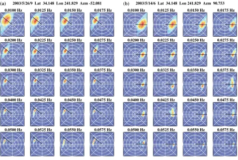
We used a simple stacking method (Aki and Richards, 1980; Johnson and Dudgeon, 1993), referenced to Pasadena station. Examples of beamforming results for frequencies between 0.01 and 0.06 Hz are shown in Figs. 2(a) and (b). The great-circle direction is shown by solid (black) line. Four concentric circles in each panel indicate the slowness of 0.1, 0.2, 0.3 and 0.4 (s/km) respectively.
Processing was done in the following way; Fourier spec-tra for the portion of time series that contain Rayleig waves were obtained first; they were obtained by using a cosine ta-pered filter. We made sure that results were not influenced strongly by a specific choice of detailed tapering range. We then used a frequency-domain beamforming approach, us-ing the Fourier spectra from each station. We referenced all spectra to Pasadena (PAS) and stacked.
A case of Rayleigh wave arrival in the northwest quadrant is shown in Fig. 2(a). The maximum peak is indicated by red and blue denotes values that are 1 dB below the peak value. Denoting the peak location (red) as (sx,sy)
(in Figs. 2(a) and 2(b)), we can estimate phase velocity by (1/
s2
x+s2y) and also its azimuth (thus deviations from
great-circle directions).
A relatively broad but single peak is seen up to about 50 mHz in Fig. 2(a). It is thus possible to determine the azimuth of arrival from the peak in the beamforming re-sults. Note that locations of the peak start to deviate from the great-circle direction at frequencies about 15–20 mHz. Deviations in this figure are systematically to the west with respect to the great-circle directions, if one viewed the in-coming waves at seismic stations. This is consistent with the particle-motion results in Fig. 1. Quantitatively, devia-tion angles from particle modevia-tion are as large as 30–40 de-grees but vary from station to station to some extent. It is similar to variations in arrival azimuth estimates, shown later in Fig. 3(b), in which the average angle is about 20 degrees but a large number of data exist between 10 and 30 degrees.
Multiple peaks, or the evidence for multipathing, are ob-vious in results for 55 mHz and 57.5 mHz. There are at least three peaks in each panel indicating three different wave packets from different azimuths. The proximity of peaks to the concentric circle for 0.3 s/km suggests that they are all fundamental-mode Rayleigh waves, arriving from multiple azimuths.
Figure 2(b) shows the case of Rayleigh-wave arrival from the east. They are generally consistent with the great-circle propagation but some panels, especially the ones at 37.5 mHz, 42.5 mHz and 47.5 mHz, show multiple peaks. The fact that these complications arise for intermediate fre-quency ranges indicate that multipathing problem is very hard to solve, even for frequencies below 50–60 mHz.
2003/5/26/9 Lat 34.148 Lon 241.829 Azm -52.081
0.0100Hz 0.0125 Hz 0.0150Hz 0.0175 Hz
0.0200Hz 0.0225 Hz 0.0250Hz 0.0275 Hz
0.0300Hz 0.0325 Hz 0.0350Hz 0.0375 Hz
0.0400Hz 0.0425 Hz 0.0450Hz 0.0475 Hz
0.0500Hz 0.0525 Hz 0.0550Hz 0.0575 Hz
(a) 2003/5/14/6 Lat 34.148 Lon 241.829 Azm 90.753
0.0100Hz 0.0125 Hz 0.0150Hz 0.0175 Hz
0.0200Hz 0.0225 Hz 0.0250Hz 0.0275 Hz
0.0300Hz 0.0325 Hz 0.0350Hz 0.0375 Hz
0.0400Hz 0.0425 Hz 0.0450Hz 0.0475 Hz
0.0500Hz 0.0525 Hz 0.0550Hz 0.0575 Hz
(b)
Fig. 2. (a) Beamforming results from 0.01 Hz to 0.0575 Hz for Rayleigh waves from the northwest quadrant. The peak value is denoted by red. Intermediate amplitudes are in yellow and small ampliudes are in blue. Great-circle directions are indicated by black lines. The peak is broad at 0.01 Hz because size of the array is small for this frequency. The peaks (red) are typically shifted to the west of black lines. Clear multipathing is seen in results at 55 mHz and 57.5 mHz. (b) Beamforming results for arrival from the east. The peak locations are mostly on the great-circle direction. Multipathing is seen in results at 37.5 mHz, 42.5 mHz and 47.5 mHz, however.
but the resolution is not good (the width of peaks is broad) due to the size of an seismic array. (3) Systematic devia-tions from great circle direcdevia-tions are seen in higher frequen-cies, in some cases starting at about 15 mHz, but typically at about 30 mHz. In most case, a single arrival azimuth can be determined. (4) However, multipathing is occasionally seen for intermediate frequencies (between 10 and 60 mHz) and its occurrence is hard to predict. We have not found any systematics in the emergence of these multipathing effects.
4
.
Proposed approach
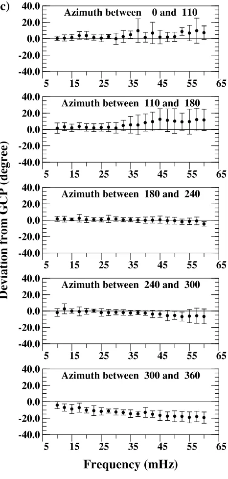
We made plots for angles of deviation from the great-circle paths for 201 events. The angles were plotted as a function of frequency for different azimuth windows. Mea-sured angles (deviations) show fair amount of scatter from event to event as two top panels in Figs. 3(a) and (b) show. These scatters might cause some problems in the analysis, if we applied the beamforming method on an event-by-event basis. On the other hand, there are clear systematics in the distributions of measured angles in both figures. We thus decided to estimate the arrival azimuth for a given azimuth window by computing the means and errors for these points. After trials and errors, we decided to divide the entire 360-degree range in five different azimuth windows. They are 0–110, 110–180, 180–240, 240–300 and 300–360 de-grees clockwise from North.
Figure 3(a) shows the results for azimuth between 180
and 240 degrees (southwest). There are many earthquakes in this range because this range includes earthquakes in the South Pacific. Deviations from the great-circle paths are generally small in this azimuth.
Figure 3(b), for the azimuth between 300 and 360 de-grees, shows the largest deviation from the great circle di-rections among the five azimuth windows. This azimuth range includes earthquakes from Alaska, Kuril, Japan and Taiwan. Rayleigh waves in this azimuth window tend to propagate at grazing angles along sharp structural contrasts in subduction zones (Kuril, Aleutian) and the continent-ocean boundaries off the coast of western United States. For this azimuth range, deviations are seen at frequencies as low as 15 mHz and seem to grow for higher frequencies and reach 20 degrees at 50 mHz.
Computed means and error bars (one sigma) are given in the bottom panels (Figs. 3(a) and (b)). Summary of results for all five azimuth windows are shown in Fig. 3(c).
As a first step, we applied the results given in Fig. 3(c). Since the plane-wave approximation seems to be accept-able, we applied corrections to the azimuth of incoming waves and measured phase velocities between pairs of sta-tions as in our previous work (e.g., Tanimoto and Prindle, 2002). Detailed analysis can be found in Prindle (2006).
-40.0 -30.0 -20.0 -10.0
0.0
10.0
20.0
30.0
40.0
5 15 25 35 45 55 65
A
zi
muth between 1
80
and 2
40
-40.0 -30.0 -20.0 -10.0
0.0
10.0
20.0
30.0
40.0
5 15 25 35 45 55 65
F
re
q
uency (m
Hz
)
D
ev
i
at
i
on from
GC
P (degree)
(a)
-40.0
-30.0
-20.0
-10.0
0.0
10.0
20.0
30.0
40.0
5 15 25 35 45 55 65
A
zi
muth between 3
00
and 3
60
-40.0
-30.0
-20.0
-10.0
0.0
10.0
20.0
30.0
40.0
5 15 25 35 45 55 65
F
re
q
uency (m
Hz
)
D
ev
i
at
i
on from
GC
P (degree)
(b)
Fig. 3. The data were divided into five azimuth windows. For each window, angles of deviation from great-circle direction as a function of frequency are plotted. Raw data are given at top and the means and standard errors are shown at bottom. Results from two windows are shown 180–240 degrees (a) and 300–360 degrees (b). (c) Summary of angle-deviations for the five windows.
-40.0 -20.0
0.0
20.0
40.0
5 15 25 35 45 55 65
Azimuth between 0 and 110
-40.0 -20.0
0.0
20.0
40.0
5 15 25 35 45 55 65
Azimuth between 110 and 180
-40.0 -20.0
0.0
20.0
40.0
5 15 25 35 45 55 65
D
ev
i
at
i
on from
GC
P (degree)
Azimuth between 180 and 240-40.0 -20.0
0.0
20.0
40.0
5 15 25 35 45 55 65
Azimuth between 240 and 300
-40.0 -20.0
0.0
20.0
40.0
5 15 25 35 45 55 65
F
re
q
uency (m
Hz
)
Azimuth between 300 and 360
(c)
Fig. 3. (continued).
scheme is based on empirical evidence that azimuth alone can be used to predict deviations angles. This situation oc-curred probably because there are only one seismically ac-tive region within a given azimuth. Therefore, this empiri-cal approach is not guaranteed to work for other regions.
5.
Impact on a
zi
muthal an
i
sotropy
-120 -118 -116 -114 32
33 34 35 36 37 38
Longitude
L
at
i
tude
Rayleigh-wave Azimuthal Anisotropy (0.045)
2.2 (%)
0.0 (%) 1.1 (%) 0.0 (%) 0.7 (%) 1.3 (%)
-120 -118 -116 -114
32 33 34 35 36 37 38
Longitude
L
at
i
tude
Azimuthal Anisotropy with Correction (0.045)
1.6 (%) 0.0 (%) 0.8 (%)
-120 -118 -116 -114
32 33 34 35 36 37 38
Longitude
L
at
i
tude
Azimuthal Anisotropy with Path Correction (0.025)
1.5 (%) 1.6 (%) 0.0 (%) 0.8 (%)
-120 -118 -116 -114
32 33 34 35 36 37 38
Longitude
L
at
i
tude
Rayleigh-wave Azimuthal Anisotropy (0.025)
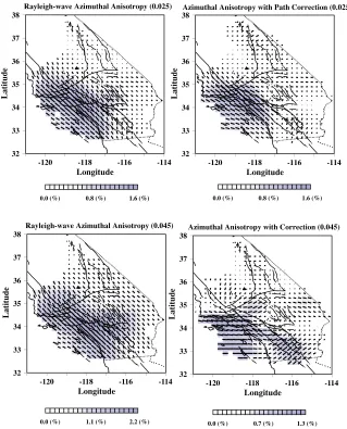
Fig. 4. Phase velocities were measured by taking into account the five-window scheme in Fig. 3(c). The most striking changes are seen in azimuthal anisotropy results at high frequencies. The left column shows the results without the correction (25 mHz at top and 45 mHz at bottom) and the right columns show results with the correction. While the changes in the results for 25 mHz are not large, directions of the fast velocity in the 45 mHz map changes dramatically. They illustrate the importance of taking into account the correct arrival azimuths in phase velocity measurements.
We solved for homogeneous block structure using ray the-ory.
Figure 4 shows our results for azimuthal anisotropy at two frequencies, 25 and 45 mHz, with and without the correction procedure we propose above. The left panels are the results without the correction (thus the great-circle path propagation) and the right panels are the results with the correction, using the five different azimuth range into consideration (Fig. 3(c)).
The results at 25 mHz, given at top, do not show ma-jor differences due to the incorporation of the beamforming results. However, at 45 mHz, the directions of fastest ve-locity azimuth change rather dramatically. On the west side of the San Andreas fault, the fastest directions are mostly northwest-southeast directions without our proposed cor-rection, but they turn out to be almost east-west after the correction. There are fewer stations off the coast, but is-lands are mostly occupied by stations, thereby giving us some resolving power even in this area. Because deviations from the great-circle paths are much larger at 45 mHz than 25 mHz, this result is most likely related to the corrections
we apply to data. It may even imply that the correct di-rections of azimuthal anisotropy cannot be recovered unless the correct arrival azimuth is taken into account in the phase velocity analysis.
This result may not be surprising since a larger devia-tion from a great-circle path tend to lead to a larger veloc-ity estimate (Pedersen, 2006). So the directions of strong great-circle deviation may tend to become a fast propaga-tion direcpropaga-tion.
6
.
C
onclus
i
on
We proposed a new Rayleigh wave analysis technique that combines the beamforming of array data (for Southern California Network) and two-station phase velocity mea-surement.
a plane-wave assumption seems to hold (to first order). We developed a specific scheme of dividing the whole azimuth into five different azimuth windows for data in Southern California. The procedure makes a large impact on the results of azimuthal anisotropy, especially for higher frequencies above 30 mHz. Since the directions of the fast velocity axes is perhaps one of the most important aspects of anisotropic structure for tectonic interpretations, correcting for the angles of deviations from great-cirle paths seems critical for surface wave analysis.
Acknowledgments. This study was supported by the Southern California Earthquake Center (SCEC). SCEC is funded by NSF cooperative Agreement EAR-0106924 and USGS Cooperative Agreement 02HQAG0008. The SCEC contribution number for this paper is 1037.
References
Aki, K. and P. G. Richards,Quantitative Seismology, W. H. Freeman and Company, San Francisco, 1980.
Baumont, D., A. Paul, G. Zandt, S. Beck, and H. Pedersen, Lithospheric structure of the central Andes based on surface wave dispersion, J. Geophys. Res.,107, B12, 2371, doi:10.1029/2001JB000345, 2002. Bourova, E., I. Kassaras, H. A. Pedersen, T. Yanovskaya, and D. Hatzfeld,
Constraints o absolute S velocities beneath the Aegean Sea from surface wave analysis,Geophys. J. Int.,160, 1006–1019, doi:10.1111/j.1365-246X.2005.02565.x, 2005.
Bruneton, M., V. Farra, H. A. Pedersen, and teh SVEKALAPKO Seismic Tomography Working Group, Non-linear surface wave phase velocity inversion based on ray theory,Geophys. J. Int.,151, 583–596, 2002. Cotte, N., H. A. Pedersen, M. Campillo, V. Farra, and Y. Cansi,
Off-great-circle propagation of intermediate-period surface waves observed on a dense array in the French Alps,Geophys. J. Int.,142, 825–840, 2000. Friedrich, W., E. Wielandt, and S. Strange, Non-plane geometries of
seis-mic surface wavefields and their implications for regional surface wave tomography,Geophys. J. Int.,119, 931–948, 1994.
Johnson, Don H. and D. E. Dudgeon,Array Signal Processing, P T R Prentice-Hall Inc., Upper Saddle River, New Jersey, 1993.
Laske, G. and G. Masters, Constraints on global phase velocity maps by long-period polarization data,J. Geophys. Res.,101, B7, 16059–16075, 1996.
McGarr, A., Amplitude variations of Rayleigh waves—Across a continen-tal margin,Bull. Seism. Soc. Am.,59, 1281–1305, 1969a.
McGarr, A., Amplitude variations of Rayleigh waves—Horizontal refrac-tion,Bull. Seism. Soc. Am.,59, 1307–1334, 1969b.
Pedersen, H. A., Impacts of non-plane waves on two-station measurements of phase velocities,Geophys. J. Int.,165, 279–287, doi:10.1111/j.1365-246X.2006.02893.x, 2006.
Pollitz, F., Regional velocity structure in nortehrn California from inver-sion of scattered seismic surface waves,J. Geophys. Res.,104, B7, 15043–15072, 1999.
Prindle, K., Souther California Surface Wave Analysis: Recovery of Three-dimensional S-wave Velocity Structure, the Finite Frequency, Off Great-Circle Propagation and Azimuthal Anisotropy,Ph.D. thesis, Uni-versity of California, Santa Barbara, 2006.
Prindle, K. and T. Tanimoto, Teleseismic Surface Wave study for S-wave velocity structure under an array: Southern California,Geophys. J. Int., 166, 601–621, 2006.
Tanimoto, T. and Don L. Anderson, Lateral Heterogeneity and Azimuthal Anisotropy of the Upper Mantle: Love and Rayleigh Waves 100–250 s,
J. Geophys. Res.,90, 842–1858, 1985.
Tanimoto, T. and K. Prindle, Three-dimensional S-wave velocity structure in Southern California,Geophys. Res. Lett., 29, 8, 1–4, doi:1029/ 2001GL013486, 2002.
Tape, C., Q. Liu, and J. Tromp, Finite-frequency tomography using adjoint methods—Methodology and examples using membrane surface waves.
Geophys. J. Int.,2006 (in press).
Yang, Y. and D. W. Forsyth, Rayleigh wave phase velocitiers, small-scale convection, and azimuthal anisotropy beneath souther California, J. Geophys. Res.,111, B07306, doi:10.1029/2005JB004180, 2006. Zhao, L. and T. Jordan, STructural sensitivity of finite-frequency seismic
waves: A full-wave approach,Geophys. J. Int.,165, 981–990, 2006.