R E S E A R C H
Open Access
The stability and bifurcation analysis of a
discrete Holling-Tanner model
Hui Cao
1*, Zongmin Yue
1and Yicang Zhou
2*Correspondence:
1Department of Mathematics,
Shaanxi University of Science & Technology, Xi’an, 710021, China Full list of author information is available at the end of the article
Abstract
A discrete predator-prey model with Holling-Tanner functional response is formulated and studied. The existence of the positive equilibrium and its stability are
investigated. More attention is paid to the existence of a flip bifurcation and a Neimark-Sacker bifurcation. Sufficient conditions for those bifurcations have been obtained. Numerical simulations are conducted to demonstrate our theoretical results and the complexity of the model.
Keywords: discrete Holling-Tanner model; flip bifurcation; Neimark-Sacker bifurcation; stability
1 Introduction
Differential equations and difference equations are two typical mathematical approaches to modeling population dynamical systems. There have been an increasing interest and research results on discrete population dynamical systems in spite of their complexity [–].
Predator-prey models describe one of the most important relationships between two interacting species and have received much attention of applied mathematicians and ecol-ogists. The stability and existence of equilibrium state, the permanence of a system, the Hopf bifurcation and the chaos of different continuous predator-prey models have been extensively investigated. However, there are less results on dynamical behaviors of dis-crete predator-prey models. The flip bifurcation and the Neimark-Sacker bifurcation are two important phenomena of discrete population model dynamics. Liu and Xiao [] used the center manifold theorem to study the flip bifurcation and the Neimark-Sacker bifurca-tion. Agizaet al.[] and Celiket al.[] used the numerical simulations to discuss the flip bifurcation and the Neimark-Sacker bifurcation. Huet al.[] also used the center manifold theorem to study the flip bifurcation and the Neimark-Sacker bifurcation.
The following continuous prey-predator model with Holling-Tanner functional re-sponse is very interesting and has been studied by many authors [–]:
dx dt =rx
– x
K
– qxy
x+a,
dy dt=ry
– y
γx
,
()
wherex(t) andy(t) are the numbers of the prey and the predator species at timet, respec-tively.randrare the intrinsic growth rates or biotic potential of the prey and predator,
respectively.Kis the prey environment carrying capacity.γ is a measure of the food qual-ity that the prey provides for conversion into predator births. qis the maximal preda-tor per capita consumption. a is the number of prey necessary to achieve one-half of the maximum rateq. The variables and parameters satisfy (x,y)∈ {(x,y)|x> ,y> }and
r,r,K,γ,q,a> .
After introducing the new variables and parameters
u= x
K, v=
y
γK, τ=rt, θ=
r r
, b= a
K, c=
qγ
r
,
system () becomes
du
dτ =u( –u) –
cuv u+b, dv
dτ =θv
– v
u
.
()
Motivated by a similar idea, we study the following discrete-time model corresponding to model ():
u(t+ ) =u(t)exp
–u(t) – cv(t)
u(t) +b
,
v(t+ ) =v(t)exp
θ
– v(t)
u(t)
,
()
whereu,v,c,b, andθ are defined as in model (). It is assumed that the initial value of solutions of system () satisfiesu() > ,v() > and all the parameters are positive. It is easy to prove that if the initial values (u(),v()) are positive, then the corresponding solution (u(t),v(t)) is positive too.
In this paper, we study the dynamical behaviors of model (). The existence and stability of the positive equilibrium are investigated in Section . The criteria for the existence of a flip bifurcation and a Neimark-Sacker bifurcation are given in Section . Numerical simulations are conducted to demonstrate our theoretical results and show the complexity of the model dynamics in Section , too. Concluding remarks and discussions are given in Section .
2 The existence and stability of the equilibrium
We firstly discuss the existence of the equilibria of model (). From model () we know that the coordinatesuandvof the positive equilibrium satisfy
–u– cv
u+b= , – v
u = , ()
which is equivalent to
Quadratic equation () has a positive solution
u∗=–(b+c– ) +
(b+c– )+ b
.
ThenE(u∗,u∗) is a positive equilibrium of model (). From the expression
u∗=–(b+c– ) +
(b+c– )+ b
=
b
b+c– +(b+c– )+ b,
we know that u∗ is a decreasing function of cwithlimc→+u∗= ,limc→∞u∗ = , and
<u∗< .
The linearized matrix of model () at the equilibriumE(u∗,u∗) is
J=
–u∗+(u∗cu+∗b) –u∗cu∗+b
θ –θ
.
The characteristic equation of matrixJish(λ) = , withh(λ) =λ–pλ+q= , where
p= –θ–u∗+ cu
∗ (u∗+b),
q= –θ–u∗+θu∗+cu∗(u∗+bθ) (u∗+b) .
Letλandλbe two solutions ofh(λ) = , and=max{|λ|,|λ|}. From the Jury criterion,
we know that the necessary and sufficient conditions for< are
+p–q> , –p+q> , –q> .
It is easy to obtain that
–p+q=θu∗+ bcθu (u∗+b) >
holds true for all positive parameters. The other two conditions become
+p+q= – θ– u∗+θu∗+ cu
∗ (u∗+b)+
bcθu∗ (u∗+b) > ,
–q=u∗+θ–uθ– cu
∗ (u∗+b)–
bcθu∗ (u∗+b) > .
()
The conditions +p+q> and –q> in () are equivalent to
(θ+ u∗– –θu∗)(u∗+b) u
∗+bθu∗ <c<
(θ+u∗–θu∗)(u∗+b)
u
∗+bθu∗ . ()
By using the equation ucu∗∗+b = –u∗ andu∗=b– (b+c– )u∗, we can have another equivalent conditions of ()
–b– u∗
–u∗ <θ< + c
Then we have the following stability theorem.
Theorem . The unique positive equilibrium point E(u∗,u∗)of model()is asymptoti-cally stable if and only if condition()or condition()holds.
Proof From the straightforward calculation, we can have the equivalent condition given in (). Here we verify the equivalence of condition () and condition (). The first inequal-ity in condition () is equivalent to
cθu∗
u∗+b> (θ– )
–u∗+ cu
∗ (u∗+b)
. ()
Substituting u∗cu∗+b= –u∗into inequality () yields
θ( –u∗) > (θ– )
–u∗+u∗( –u∗)
u∗+b
. ()
Inequality in () is equivalent to
u∗+b+ ( –u∗)(u∗+b)>θ u∗+b+ ( –u∗)u∗. ()
Using the equalityu
∗=b– (b+c– )u∗in () leads to
u∗( +b+ c) >θ( +b+c)u∗. ()
It follows from () that
θ<( +b+ c) +b+c) = +
c
+b+c. ()
The second inequality in () is equivalent to
( –θ)
–u∗+ cu
∗ (u∗+b)
< – cθu∗
u∗+b. ()
Substituting u∗cu+∗b= –u∗into inequality () yields
( –θ)
–u∗+u∗( –u∗)
u∗+b
< –θ( –u∗). ()
Inequality in () is equivalent to
u∗( –u∗) –u∗(u∗+b) <θ( –u∗)u∗. ()
From inequality () and <u∗< it follows that
θ> –b– u∗
–u∗ . ()
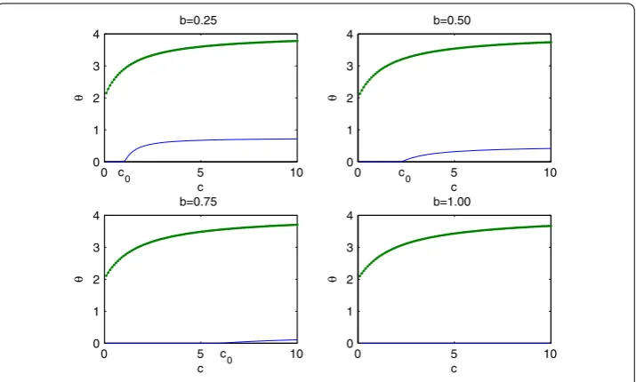
Figure 1 The stability domain of the equilibriumE(u∗,u∗) of model().
Remark Inequality () or () gives stability conditions for the equilibriumE(u∗,u∗) of model (). Inequality () is directly obtained from (), but it is not easy to verify sinceu∗ is dependent onc. As stated in the proof of Theorem ., inequality () is easy to verify though it is difficult to obtain.
Remark When –b– u∗< , equivalent to ( –b)c< ( +b), the inequalityθ>–b–u∗
–u∗ holds true automatically. The stability condition becomesθ< ++bc+c, which is easy to verify.
Forb=,b= ,b= , andb= , the stability domain in thec–θ plane is shown in Figure . The horizontal and vertical coordinates are the parameterscandθ, respectively. For any givenc, the positive equilibriumE(u∗,u∗) is stable whenθ is between two given curves. There existscfor the subplots withb=,b=, andb=, respectively. When c<c, the positive equilibriumE(u∗,u∗) of model () is stable for <θ< ++bc+c. When
c>c, the positive equilibriumE(u∗,u∗) of model () is stable for––b–u∗u∗<θ< +b+cc+.
From conditions given in Theorem . we know that the positive equilibriumE(u∗,u∗) of model () is locally stable if –b–u∗
–u∗ <θ< +
c
b+c+. The numerical simulations
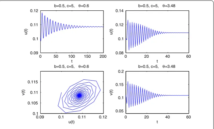
demon-strate that the positive equilibrium E(u∗,u∗) of model () may be globally asymptoti-cally stable if the conditions in Theorem . hold. If we take b= . and c= , then
E(., .) is the positive equilibrium of model (). The stability condition be-comes . <θ < .. If we take θ = ., then λ=λ¯= . + .iare the
complex eigenvalues of the linearized matrixJ of model () at the positive equilibrium
E(., .).E(., .) is a stable focus. For the initial valueu() = . and
v() = ., the solution series ofu(t) and the phase portrait are given in Figure (the left column of subplots). If we takeθ = .., thenλ= –. andλ= –. are
the real eigenvalues of the linearized matrix J of model () at the positive equilibrium
Figure 2 The stability of the equilibriumE(u∗,u∗) of model().
of subplots). The solution series and the phase portrait in Figure show that the positive equilibriumE(., .) of model () may be globally asymptotically stable.
3 Bifurcation
Bifurcation may lead to different dynamical behaviors of a model when parameters pass through a critical values. Bifurcation usually occurs when the stability of an equilibrium changes. In this section, we discuss the flip bifurcation and the Neimark-Sacker bifurcation of model ().
3.1 Flip bifurcation
We defineθ∗= +b+cc+. The stability analysis in Section shows that the positive equilib-riumE(u∗,u∗) has an eigenvalue – whenθ=θ∗, which meansE(u∗,u∗) is non-hyperbolic. The flip bifurcation may occur in the neighborhood of the endemic equilibriumE(u∗,u∗) whenθ passes through the critical pointθ∗.
The linearization matrix of model () at the equilibrium pointE(u∗,u∗) withθ=θ∗is
A=
–u∗+(u∗cu+∗b) –
cu∗ u∗+b +b+cc+ – –b+cc+
,
and the characteristic equation of matrixAisλ+p∗λ+q∗= , where
p∗=(u∗+b– )u∗
u∗+b +
c b+c+ ,
q∗= ( –u∗)
– u∗
u∗+b
+ c
b+c+
.
The eigenvalues of matrixAareλ= – andλ=(b++c)(bb++cc)+b–b(+u∗b++bc)with|λ| = . The
Theorem . Ifβ = ,then model()will undergo a flip bifurcation at E(u∗,u∗)when
θ =θ∗.That is,there exists a stable period two cycle ifθ∗<θ <θ∗+ε,whereεis a small positive number,andβis defined in the end of the proof.
Proof In order to use the center manifold theory, we treatθ as a state variable. The trans-formationsu˜=u–u∗,v˜=v–u∗, andθ˜=θ–θ∗take model () into the form
We define the matrix
The transformation
takes model () to
b=
From the center manifold theory of discrete system we know that there exists a local man-ifold of model () []. The local manman-ifold has the following expansion:
v(t) =hu(t),θ(t)
After substituting the expansion into model () and using the invariant property of the local manifold, the straightforward and careful calculation givesm=m=m=m= ,
From the second equation of model () we know thatθ(t) is always constant. Therefore, the one dimensional model induced by the center manifold is
+(λ– +θ∗)(θ∗– )b θ∗( +λ)
mθu
+θ∗– +λ
–a+
λ– +θ∗
θ∗ b
mθu. ()
It is not difficult to verify thatG(,θ) = ,∂G∂(,)u = –, and
∂G(, ) ∂u∂θ
=(λ– +θ∗)(θ∗– ) θ∗( +λ)
b= –
u∗( +b+c)
u∗( +b+ (b+c)( +b+ c)) – bc< ,
β=∂
G(, )
∂u = –
(θ∗– ) +λ
–a+
λ– +θ∗
θ∗ b
= .
Therefore, model () will undergo a flip bifurcation atE(u∗,u∗), and the bifurcation
so-lution of period two is stable (unstable) whenβ< (β> ) [].
We use numerical simulation to demonstrate the flip bifurcation of model (). When parameter valuesb= andc= are taken, then the positive equilibrium of () isE(√ – ,√ – ), the critical value ofθ∗= . The positive equilibriumE(√ – ,√ – ) is stable when <θ< .E(√ – ,√ – ) is unstable ifθ> . The calculation shows that
G(u,θ) = –u– .θu+ .u(t) + .θu+ .θu(t)
– .θu(t) – .u(t) – .u(t) – .θu
– .θu+ .θu+o ρ
.
Further calculation shows that
G(,θ) = ,
∂G(, ) ∂u
= –, ∂
G(, )
∂u∂θ
= –. < ,
β=∂
G(, )
∂u = –×. < .
From Theorem . we know that there exists a flip bifurcation of model () whenθ∗<θ< θ∗+ε, and the period two cycle is stable. The numerical simulation shows that the period
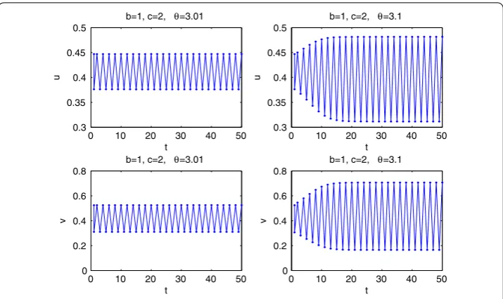
two cycle of model () may be globally asymptotically stable whenθ>θ∗andθ–θ∗is small. Figure shows the flip bifurcation of model () and its stability. For the subplots in the left column, the parameters are b= , c= , and θ = .. E(., .) and E(., .) are two points at the period two cycle of model () for those
param-eters. The solution of model () with initial conditionsu() = .,v() = . tends to the period two cycle. For the subplots in the right column, the parameters areb= ,
c= , andθ = ..E(., .) andE(., .) are the period two cycle of
model () for those parameters. The solution of model () with the same initial conditions
Figure 3 The flip bifurcation of model()from the equilibrium pointE(u∗,u∗).
3.2 Neimark-Sacker bifurcation
The Neimark-Sacker bifurcation for the discrete models is similar to the Hopf bifurcation of continuous models. In this subsection we discuss the existence of the Neimark-Sacker bifurcation of model ().
Theorem . If α = , then model () will undergo a Neimark-Sacker bifurcation at E(u∗,u∗)whenθ=––b–u∗u∗ with –b– u∗> ,whereαis defined in the proof.
Proof Letu(t) =u(t) –u∗ andv(t) =v(t) –u∗, then the equilibriumE(u∗,u∗) is trans-formed into the origin, we have
⎧ ⎨ ⎩
u(t+ ) = (u(t) +u∗)exp( – (u(t) +u∗) –uc(v(t)+(t)+u∗u∗+b)) –u∗,
v(t+ ) = (v(t) +u∗)exp(θ( –uv((tt)+)+uu∗∗)) –u∗.
()
The Taylor expression of model () at (u(t),v(t)) = (, ) to the third order is
⎧ ⎨ ⎩
u(t+ ) =(b+u∗c)+u∗b–bu(t) – ( –u∗)v(t) +P(u,v),
v(t+ ) =θu(t) + ( –θ)v(t) +P(u,v),
()
where
P(u,v) =
(c– – (b+ c)(b+ u∗))u∗ (u∗+b) u
+
(b+ c)u∗– (b+c)
u∗+b uv+
c( –u∗) (u∗+b)v
+( –u∗)[b+ ( –b– c)u∗] + ( –b– u∗)
[b+ ( +b+ c)u
∗]
(u∗+b) u
+[c–u∗( –u∗)] + ( –b– u∗)[( –u∗)( +b+ u∗) – c]
(u∗+b) u
v
+c[c– ( –u)( +b+ u∗)] (u∗+b) uv
–
c( –u
∗) (u∗+b)v
+o
P(u,v) =
straightforward calculation yield that
+[c–u∗( –u∗)] + ( –b– u∗)[( –u∗)( +b+ u∗) – c]
From Theorem .. of [] we know that the existence of a Neimark-Sacker bifurcation can be determined by the quantityα, where
α= –Re
Using the Neimark-Sacker bifurcation theorem in [], we obtain that there exists a
Neimark-Sacker bifurcation whenα= andθpasses throughθ.
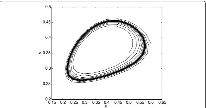
equi-Figure 4 The Neimark-Sacker bifurcation of model()at the equilibrium pointE2.
librium of () isE(., .), the critical valueθ= .. Whenθ =θ, model ()
will undergo a Neimark-Sacker bifurcation atE(u∗,u∗) (see Figure ).
4 Conclusion and discussion
The predator-prey model with Holling-Tanner functional response can give better predic-tion for some interacting species. The model also exhibits more complicated dynamics. We have studied the dynamical behaviors of a discrete prey-predator model with Holling-Tanner functional response. We have obtained sufficient conditions for the stability of the positive equilibrium, the existence of a flip bifurcation and a Neimark-Sacker bifurcation. The numerical simulations show that the model possesses more complicated dynamics. For example, if we takec= ,b= , then the positive equilibrium isE(√ – ,√ – ). The stability condition ofE(√ – ,√ – ) is <θ< . The numerical simulation shows that model () undergoes a process from periodic doubling to chaos (see Figure ).
The horizontal axis in Figure is the parameterθ, and the vertical axis is the limiting points ofu(t). When <θ < , there is only one limiting point ofu(t), which is the value of the positive equilibrium. When <θ< ., the positive equilibrium loses its stability and a stable period two cycle appears. When . <θ< ., the period two cycle loses its stability and a stable period four cycle appears. The period doubling process continues to chaos asθincreases. The top-left subplot shows a complete bifurcation. Three different domains, [., .]×[., .], [., .]×[., .], and [., .]×[., .], in the bifurcation figure are enlarged and displayed in the other three subplots. Especially, from the bottom-left subplot we can see that there is a stable period three cycle of model ().
simu-Figure 5 Model()may exhibit a process from period doubling to chaos.
lations do not give any information on the existence of two invariant closed curves. We expect that some analytical results can be obtained on those problems in the future.
Competing interests
We all authors declare that we have no competing interests.
Authors’ contributions
YZ is responsible for the model formulation and study planning. HC and ZY have done the calculation, the proof, the simulation and the application. All authors have read and approved the final manuscript.
Author details
1Department of Mathematics, Shaanxi University of Science & Technology, Xi’an, 710021, China.2Department of Applied
Mathematics, Xi’an Jiaotong University, Xi’an, 710049, China.
Acknowledgements
This study was supported by NSFC grant 11301314, by Shaanxi Provincial Education Department grant 2013JK0599, and by Doctoral Research Foundation of Shaanxi University of Science & Technology grant BJ12-20.
Received: 12 June 2013 Accepted: 16 October 2013 Published:19 Nov 2013
References
1. Liz, E, Tkachenko, V, Trofimchuk, S: Global stability in discrete population models with delayed-density dependence. Math. Biosci.199, 26-37 (2006)
2. Agiza, HN, Elabbasy, EM, El-Metwally, H, Elsadany, AA: Chaotic dynamics of a discrete prey-predator model with Holling type II. Nonlinear Anal., Real World Appl.10, 116-129 (2009)
3. Elsadany, AA, El-Metwally, HA, Elabbasy, EM, Agsia, HN: Chaos and bifurcation of a nonlinear discrete prey-predator system. Comput. Ecol. Softw.2(3), 169-180 (2012)
4. Hu, Z, Teng, Z, Zhang, L: Stability and bifurcation analysis of a discrete predator-prey model with nonmonotonic functional response. Nonlinear Anal., Real World Appl.12, 2356-2377 (2011)
5. Liu, X, Xiao, D: Complex dynamic behaviors of a discrete-time predator-prey system. Chaos Solitons Fractals32, 80-94 (2007)
6. Celik, C, Duman, O: Allee effect in a discrete-time predator-prey system. Chaos Solitons Fractals40, 1956-1962 (2009) 7. May, RM: Stability and Complexity in Model Ecosystems. Princeton University Press, Princeton (1973)
8. Sáez, E, González-Olivares, E: Dynamics of a predator-prey model. SIAM J. Appl. Math.59, 1867-1878 (1999) 9. Tanner, JT: The stability and the intrinsic growth rates of prey and predator populations. Ecology56, 855-867 (1975) 10. Wollkind, DJ, Collings, JB, Logan, JA: Metastability in a temperature-dependent model system for predator-prey mite
outbreak interactions on fruit flies. Bull. Math. Biol.50, 379-409 (1988)
11. Braza, PA: The bifurcation structure of the Holling-Tanner model for predator-prey interactions using two-timing. SIAM J. Appl. Math.63(3), 889-904 (2003)
13. Grandmonet, JM: Nonlinear difference equations, bifurcations and chaos: an introduction. Res. Econ.62, 120-177 (2008)
14. Guckenheimer, J, Holmes, P: Nonlinear Oscillations, Dynamical Systems, and Bifurcations of Vector Fields. Springer, New York (1983)
10.1186/1687-1847-2013-330