R E S E A R C H
Open Access
Optimal number of routing paths in multi-path
routing to minimize energy consumption in
wireless sensor networks
Davut Incebacak
1*, Bulent Tavli
2, Kemal Bicakci
2and Ay¸segül Altın-Kayhan
2Abstract
In wireless sensor networks, multi-path routing is proposed for energy balancing which prolongs the network lifetime as compared to single-path routing where utilization of a single route between a source node and the base station results in imbalanced energy dissipation. While it is evident that increasing the number of routing paths mitigates the problem of energy over-utilization in a subset of nodes acting as relays, the net effect of the proliferation of multiple routing paths on energy balancing remains unclear. It is imperative to keep the number of routing paths as low as possible without significantly deteriorating the network lifetime; therefore, determination of the optimal number of routing paths in multi-path routing by considering the tradeoff in routing complexity and network lifetime extension is an interesting research problem. In this study, to investigate the impact of the number of routing paths in
multi-path routing on network-wide energy balancing under optimal operating conditions, we build a novel mixed integer programming framework. We explore the parameter space consisting of a number of paths, number of nodes, maximum transmission range, network area, and network topology. The results of the analysis show that by utilizing the optimization scheme proposed, it is possible to achieve near-optimal energy consumption (within 1.0% neighborhood of the case where no restrictions are imposed on the number of routing paths in multi-path routing) using at most two paths for each node.
1 Introduction
Optimization of energy expenditure (e.g., energy-efficient routing) is one of the most important design goals in the wireless sensor network (WSN) system design [1]. In WSNs, routing protocols discover and maintain paths between sensor nodes and the base station. The data of a sensor node is conveyed towards the base station on a single path or on multiple paths. By distributing the rout-ing burden on multiple paths as opposed to transmittrout-ing on only a single path, multi-path routing leads to a more balanced energy dissipation in the network. There are sev-eral protocols designed for multi-path routing in WSNs [2-7]. The common goal of these protocols is to improve the energy efficiency of the network through multi-path routing. Additionally, they provide other capabilities (e.g.,
*Correspondence: idavut@metu.edu.tr
1Middle East Technical University, Ankara 06800, Turkey Full list of author information is available at the end of the article
intrusion detection [2], renewable energy [3], mobile sen-sors [4], fault tolerance [5], quality-of-service [6], and security [7]).
Earlier studies revealed that multi-path routing improves the energy efficiency of WSNs; however, the impact of the number of paths on the level of energy efficiency is not well understood (i.e., what amount of energy efficiency improvement should be expected with each additional path?). As the number of paths increases, so does the complexity of the routing protocol. Hence, it is desirable to limit the number of paths at some point if a further increase does not improve energy efficiency significantly, yet an analysis of the impact of limiting the number of paths on energy efficiency has not been performed in the literature.
In this study, an optimization scheme to minimize the energy consumption of sensor nodes under multi-path
routing is proposed. In fact, our main goal is to investigate the impact of multi-path routing on energy consumption characteristics of sensor nodes in WSNs. By developing a novel problem formulation using mathematical pro-gramming, we capture the essence of both routing and energy dissipation characteristics of multi-path routing. We analyze the impact of limiting the number of routes from the energy efficiency perspective within a general framework and without considering any specific proto-col or algorithm. This approach abstracts us away from the protocol-specific overhead or implementation details. Characterization of the impact of limiting the number of routes on energy balancing in WSNs is a novel research contribution and may provide valuable insights for the design of future protocols.
There are several related concepts in this area which can also be referred as multi-path routing and may be confused with the meaning of multi-path routing as it is used in this paper. In this paper, we use the term multi-path routing for partitioning the data into groups of data packets without employing data redundancy and send-ing each group of packets via a different path towards the base station. Alternate path routing is different from multi-path routing in the sense that a single path is used in normal operation, but alternative paths are kept ready to be used in case the primary path becomes unavailable. Redundant multi-path routing is another related term that means the data to be conveyed to the base station is trans-ported via multiple paths with added redundancy (e.g., multiple replicas of the data are sent on different paths) [8].
Mathematical programming is a powerful tool utilized in many studies to analyze different aspects of WSNs [9]. Here, we briefly overview the previous work most relevant to our work. In [10], a mixed integer programming (MIP) framework is proposed to analyze capacity and energy consumption of IEEE 802.15.4 cluster-tree hierarchy for organizing transmissions to provide the optimal solution for the network capacity. In [11], the problem of mini-mizing the network cost through the minimum number of relay-station installation in continuous data-gathering WSNs is investigated by using an MIP model. In [12], an MIP-based framework for optimizing the placement of RF chargers used for energy harvesting in WSNs is proposed. In [13], two joint routing and scheduling algorithms which minimize the data delivery latency while enhancing the energy efficiency in WSNs are proposed and investi-gated through an MIP framework. In [14], the impact of limiting the number of incoming and outgoing links of nodes on the network lifetime is formulated as an MIP problem.
We introduce the MIP model for multi-path routing in Section 2. Section 3 presents the results of numerical analysis. Conclusions are drawn in Section 4.
2 Model
In our framework, we make the following assumptions:
1. The network consists of stationary nodes (both sensor nodes and the base station).
2. For a substantial amount of time (epochs), topology discovery and route creation operations are not repeated [1].
3. Network reorganization period is long enough; therefore, the energy costs of topology discovery and route creation operations constitute a small fraction (e.g., less than 1.0% [15]) of the total network energy dissipation. Hence, routing overhead can be neglected in stationary WSNs without leading to significant underestimation of total energy dissipation. 4. A time division multiple access (TDMA)-based
media access control (MAC) layer is in operation which mitigates interference between active links through a time slot assignment algorithm which outputs a conflict-free transmission schedule. A combinatorial interference model can be used to model interference, and scheduling constraints can then be modeled by a conflict graph [16,17]. In [18], it is shown that such an algorithm is possible; hence, collision-free communication is achieved if sufficient bandwidth requirements are satisfied. In fact, in our model, we use a modified version of the sufficient condition presented in [18]. Furthermore, it is also possible to reduce data packet collisions to negligible levels in practical MAC protocols designed with a dynamic TDMA approach [19,20].
5. Energy dissipation for idle listening or overhearing in promiscuous mode is negligible. There are many intelligently designed MAC protocols for wireless networks that avoid energy waste in these modes [19,21]. We assume such a MAC layer is used in our framework.
6. The transmission energy model is such that the bit error rate (BER) is constant and the same for all links [22-24].
In our network model, there is a single base station and there are N sensor nodes in the network. Time is organized into rounds with durationTrnd, and the total number of rounds is Mrnd. Each sensor node-i creates the same number of data packets (si) with packet length
LP bits at each round to be conveyed to the base station (i.e., sensor nodes create CBR flows). The network topol-ogy is represented by a directed graph,G=(V,A), where
Vis the set of all nodes including the base station as node-0 andA = {(i,j) : i ∈ W,j ∈ V−i, dij ≤ Rmax}is the
ordered set of arcs. We also define setW which includes all nodes except node-0 (i.e.,W =V\ {0}). Note that we use the expression ‘node-i’ when it is used in a sentence; however, we use only ‘i’ when it is used within a mathemat-ical expression or when we need to refer to the indices of mathematical expressions in the narrative. The definition ofAimplies that no node sends data to itself or to a node that is separated from it beyond the maximum transmis-sion rangeRmax. The distance between node-iand node-j
is denoted bydij. Each node can forward its generated data towards the base station using at mostNP paths. Differ-ent paths can be either disjoint or braided (i.e., two paths can share common links in their chains of links form-ing paths). Data generated at node-k forwarded on the
lth path flowing from node-ito node-jis represented as
fijkl. Moreover,blk is the total amount of data packets gen-erated by node-k (k ∈ W) and transmitted on the lth configuration to the base station, andaklij indicates if arc
(i,j)∈Ais used in thelth routing configuration originated at node-k(k∈W).
We adopt the energy model used in [27]. In this model, the amount of energy to transmit LP bits of data is
Etx,ij(LP) = LP(ρ +εdαij) and to receiveLP bits of data is
Erx(LP)= LPρ, whereρrepresents the energy dissipated in the electronic circuitry,εdenotes the transmitter effi-ciency, andα represents the path loss exponent. Packet error rate isχ=(1−(1−ϕ)LP), whereϕis the BER. Each packet has to be transmittedλ=1/(1−χ )times (average packet retransmission rate), on the average, for success-ful delivery of the packets. The interference range of a transmission from node-ito node-jisγdij, whereγ is the interference range multiplier [18]. To model interference between links, we define a binary interference matrix,Iijm, presented in Equation 1. If node-i is in the interference region of the transmission from node-jto node-m(i.e.,
γdjm ≥ dji), then node-iis blocked from receiving any data because any such flow to node-iresults in a conflict (packet collision). Therefore, ifIjmi =1, then node-ihas a conflict with the flow on arc(j,m)(node-iis sharing the bandwidth with the flow on arc(j,m)). On the other hand, ifIjmi = 0, then flow on arc(j,m)is not conflicting with node-i. Generally speaking, the interference range is equal to or greater than the transmission range (i.e.,γ ≥ 1) [18,28]. This means that depending on the value of γ,
node-j’s transmission to node-mcan interfere with
node-ieven if the distance between node-jand node-mis less than the distance between node-jand node-i.
Ijmi =
1 ifγdjm≥dji∀j∈W,∀m∈V\ {j}
0 otherwise (1)
The objective of the optimization problem is to mini-mize the the maximum energy requirement (E) of sensor nodes. The network flow is modeled in the form of a series of constraints presented in the MIP model for multi-path routing (below). All system variables with their acronyms and descriptions are presented in Table 1.
Table 1 Terminology for MIP formulation
Variable Description
N Number of nodes
fkl
ij Number of data packets generated at node-kforwarded on
thelthpath flowing from node-ito node-j
si Number of data packets generated at node-i
Erx(LP) Energy consumption for receivingLPbits of data
Etx,ij(LP) Energy consumption for transmittingLPbits of data from
node-ito node-j
dij Distance between node-iand node-j
ρ Energy dissipated in the electronic circuitry
ε Transmitter efficiency
α Path loss exponent
E Battery energy of each sensor node
G=(V,A) Directed graph that represents network topology V Set of nodes, including the base station as node-0
W Set of nodes, except the base station (node-0)
A Set of edges (links)
l Set of paths
akl
ij Binary variable to determine if arc (i,j)∈Ais used in the
lth routing configuration originated at sensork∈W. bl
k Total amount of data sensed by sensork∈Wand
transmitted on thelth configuration to the base station
R Radius of deployment area
Rmax Maximum transmission range
Np Number of paths
LP Packet length in bits
Mrnd Number of rounds
Trnd Round duration
ξ Channel data rate (bits/s)
γ Interference range multiplier
ϕ BER (bit error rate)
χ Packet error rate
MinimizeE
Constraint (2) limits the energy used by each sensor node for data transmission and reception by the total battery energy allocated to it. In fact, the objective is to minimize the energy dissipation of the maximum energy dissipating sensor node. The expression in the parenthesis gives the energy dissipation of node-ion packet transmis-sion and reception for conveying source node-k’s data on its lth routing path. Summation over k and l gives the total energy dissipation of node-i. Energy dissipation for retransmissions are incorporated into the model through the multiplication of the whole expression byλ. If there is no retransmission, thenλ=1. The energy model we used [27] enables the adjustment of transmission energy for each node pair to enable a uniform signal-to-noise ratio (SNR) at each receiver.
Constraint (3) is known as the flow conservation con-straint, which is satisfied for alli(all nodes including the base station),k (sensor nodes), and l (routing paths). If node-i is the source node (i = k), then the difference between the sum of outgoing flows and the sum of incom-ing flows is the total amount of packets injected into the network by source node-kon itslth routing path (blk). If
i = 0 (the base station), then the all packets generated at each node-kand transmitted on path-l(blk) reach the base station. Ifi=kandi=0, then the sum of incoming flows is equal to the sum of outgoing flows (node-i is a relay node for source node-k’s flow on its lth path). In sum-mary, constraint (3) ensures that all flow generated at each node-kand transmitted on path-lreach the base station.
Constraint (4) ensures that data generated at sensor node-k and routed out to the rest of the network does not loop back to node-k. In other words, the sum of flows generated at node-k and received by node-k itself is 0. Note that constraint (10) ensures that all flows are non-negative; hence, constraint (4) together with con-straint (10) dictates that the value of any flow creating any possible loop is exactly 0.
Constraint (5) guarantees that each node-k (k ∈ W) generates and sends exactly a total of skMrnd packets to the base station. The total amount of data packets gen-erated at node-kis routed to the base station by using at mostNP paths, and the amount of data injected by
node-kinto each one of the paths is denoted asblk; hence, the summation overlfor eachkgives the total amount of data generated at node-k. Since both the flows and the amount of data injected on each path are integer variables, the packets cannot be split (all packets are created asLP bits long and reach the base station with the same length as they are formed). However, different paths can be used in a periodic time interleaved fashion. It is also possible that different paths are used to convey data in an aperiodic sequential arrangement. For example, if sk = 1 packet,
Mrnd = 3, 600 rounds,NP = 3 paths,b15 = 1, 800
pack-ets, b25 = 1, 200 packets, and b35 = 600 packets, then node-5 can create a cyclic structure with a length of six rounds. At each cycle of six rounds, three data packets, two data packets, and one data packet are conveyed to the base station using the first path, the second path, and the third path, respectively. Alternatively, node-5 can convey all its data from round 1 to round 1,800 on its first path, from round 1,801 to round 3,000 on its second path, and from round 3,001 to round 3,600 on its third path. In our model, we do not impose any timing restric-tion on scheduling. We determine the optimal paths and the amount of data transported on each path through-out the entire network operation as specified byNP, sk,
Constraint (6) ensures that an arc(i,j)∈Ais marked as used for conveying data generated at node-kon itslth path only if there is positive flow on(i,j)∈A(aklij =1 iffijkl>0). Note that the value offijkl can at most beskMrnd. Such a case happens if node-k uses only one routing path (i.e.,
b1k = fijk1andbkm = 0 form> 1). Iffijkl = 0, then binary variableaklij can be either 1 or 0 (i.e., by itself constraint (6) does not forceaklij to neither 1 nor 0 forfijkl=0). However, constraint (7) as described below forcesaklij to be 0 if both options are feasible. Hence, constraint (6) in conjunction with constraint (7)results inaklij =0 iffijkl =0.
The flow on each configuration is guaranteed to be non-bifurcated by constraint (7). Note that constraint (7) must be satisfied for all values ofi,k, andl. Consider one of the possible combinations:(i,k,l) = (3, 3, 1). For this exam-ple, constraint (7) states that data generated at node-3 which is designated to flow on its first routing path trans-mitted by node-3 (the first hop of the path) can have only one receiver (i.e., there should be only one second hop node, which can be the base station or another node acting as a relay). The summation over arc set(3,j)guarantees that only one of the arcs(3,j)have non-zero flow because the sum is equal to or less than 1. In the same example, assume that j = 7 (i.e., f3731 = b13 andf331m = 0 for all
m=7). As the second hop relay, node-7 can transmit the data it received from node-3 (f3731) to only one of its neigh-bors (dictated again by constraint (7)). If the third hop relay is node-8, thenf7831 = f3731 = b13andf731m = 0 for all
m=8. Continuing in this manner, data injected by source node-3 to its first path reaches the base station without being split into multiple branches. In other words, con-straint (7) enables the construction of an unbroken and non-branching logical pipe (path) from the source to the base station for transportation of data. Indeed,NP is the upper limit on the number of such pipes for each source node. The maximum number of such pipes in a network ofMsensor nodes can beMNP.
Constraint (8) is used to have a logical ordering of the configurations for originator nodes. Constraint (8) implies thatb1k≥b2k≥b3k≥. . .≥bNP
k (i.e., the number of packets conveyed on thelth path of source node-kis greater than or equal to the number of packets conveyed on its(l+1)th path).
To address bandwidth limitations in a broadcast medium, we need to make sure that the bandwidth used to transmit and receive at each node is limited by the available channel bandwidth. Such a constraint should take the shared capacity into consideration. For node-i, we refer to the flows around node-i which are not flowing into or flowing out of node-i but affecting the available bandwidth available to node-i as interfer-ing flows. Constraint (9) guarantees that for each node (including the base station), the aggregate amount of
incoming flows, outgoing flows, and interfering flows can be scheduled within the given time frame (Trnd sec-onds/round × Mrnd rounds = TrndMrnd seconds). The summation over l, k, (i,j), and (j,m) gives the total number of packets sharing the capacity of node-i. Mul-tiplication by LP (bits/packet) converts the number of packets to number of bits. Division by ξ (channel data rate – bits/second) transforms number of bits to seconds. Scaling withλis for the extra time needed due to retrans-missions. This constraint is a modified version of the sufficient condition given in [18]. We note that in the numerical analysis, we choose the parameters affecting constraint (9) in such a way that the maximum value of the left-hand side of the inequality is more than an order of magnitude lower than the right-hand side value; there-fore, construction of a conflict-free transmission schedule through a non-complicated time-slot assignment algo-rithm is possible. It is also shown that well-designed carrier sense multiple access (CSMA)-based MAC proto-cols are highly successful in reducing the collision rate to negligible levels provided that the network traffic is much lower (e.g., an order of magnitude) than the available capacity [29,30].
Finally, constraint (10), constraint (11), and constraint (12) are nonnegativity constraints for the variables of the model.
The objective is to minimizeE, which is the energy of the battery in each node. Once the parameterNPis set, the solution of the model gives the set of paths each node uses to forward its data and the amount of data transported on each of these paths in a way that the energy required by the most energy consuming node is minimized. As a result, all nodes transmit their data in order to keep the required battery energy per sensor node as low as possi-ble. In other words, all nodes dissipate their energies in the most balanced fashion. Sensor nodes are not required to use exactlyNP paths (e.g., it is possible for a node to use only two paths for transporting all its generated data even ifNP >2). Furthermore, the amount of data flow on each path (blk) is also determined by the MIP framework to optimize energy dissipation.
3 Analysis
As we have mentioned, general MIP models are com-putationally difficult problems. They are in NP-hard class according to their computational complexity [32]. Although there are some MIP problems with efficient optimization property (i.e., they can be solved relatively easier due to their special structures), we are not aware of any previous result on the applicability of such a prop-erty in our problem. Our preliminary tests show that the LP relaxation of the problem obtained by relaxing the integrality constraints on binary variables does not pro-vide the same optimal solution with the original MIP model and the gap is actually significant in many cases. Moreover, the solution times increase significantly as the instance sizes get larger. Hence, even for medium-sized instances, the solution times can be quite high, which can be mitigated using several implementation heuris-tics. Since our motivation in this paper is to explore the impact of multi-path routing rather than develop-ing specialized efficient solution algorithms for the prob-lem, we accept solutions with a relative gap of no more than 1.0%.
Suppose that we have a solution satisfying all integer requirements and have the best objective function value (zB) found so far. Then, the relative gap for this solution measures the distance betweenzBand the available best bound for the optimal objective function value (zL) using the ratio |zBz−LzL|. LP-based branch-and-bound algorithms are used for solving MIPs in GAMS [31]; thus, zL is the LP relaxation solution of the MIP problem under consid-eration. Note that, in general,zLis not a feasible solution because integer variables are treated as continuous vari-ables (i.e., the occurrence of non-integer values for binary variables is allowed in zL). The acceptable relative gap can be controlled via the parameteroptcrin GAMS, and when it is set to 0.0, the solution algorithm stops with the exact optimal solution. In this study, we letoptcr=1.0%, which provides significant time savings in exchange for an immaterial sacrifice for optimality.
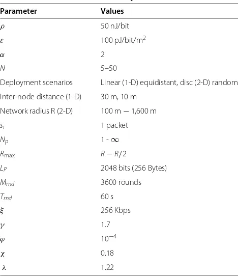
In our analysis, we investigate two deployment scenar-ios: (1) linear deployment in which nodes are deployed equidistantly on a line without any randomness and (2) uniform random distribution in which N nodes are deployed in a disc of radiusR. There are many applications for linear sensor network deployments including bor-der surveillance, highway traffic monitoring, safeguard-ing railway tracks, oil and natural gas pipeline protection, structural monitoring, and surveillance of bridges and long hallways [33]. We assume that there is a single base station located at one end in linear deployments and at the center in disc deployments. The communication parame-ters are chosen asε = 100 pJ,ρ = 50 nJ, andα = 2, the same as the ones in [27]. For random deployment sce-narios, each problem is solved for 100 random topologies,
and the results are averaged. The parameters used in the analysis are presented in Table 2.
A small-scale WSN topology is presented in Figure 1 to illustrate the network dynamics clearly. We prefer line topology to avoid more complex flow patterns in Figure 1. The numbers on each arc show the fraction of the total amount of data generated at each sensor node. For exam-ple, f5053 = 0.23 shows that f5053 = 0.23 × λ × s5 × Mrnd packets, which is equal to 1,010 packets; further-more, it also shows that b15 = 1, 010 packets. Nodes are placed on a line with 30 m separation andRmax = 150 m.
Base station is node-0. The MIP model is solved with(a) NP → ∞, (b) NP = 2, and(c) NP = 1. Energy dis-sipations are indicated near the nodes. When there is no limit on the number of paths used by each sensor node (NP → ∞), the required battery energy for each node is 5.86 J (i.e., energy dissipations of all nodes are exactly bal-anced). For the optimal case, node-4 and node-5 use three paths and other nodes use a single path. When the num-ber of paths used by each sensor node is upper limited by 2 (NP = 2), the required energy for each sensor node becomes 5.87 J (i.e., percentage energy overhead is 0.14% with respect to theNP → ∞case). Note that all sensor nodes spend the same amount of energy; however, energy dissipation is slightly higher than theNP → ∞case due to the suboptimal path selection.
For the case ofNP = 1 (i.e., single-path routing), energy overhead becomes 21.30% when compared to theNP →
Table 2 Parameters used in analysis
Parameter Values
ρ 50 nJ/bit
ε 100 pJ/bit/m2
α 2
N 5–50
Deployment scenarios Linear (1-D) equidistant, disc (2-D) random
Inter-node distance (1-D) 30 m, 10 m
Network radius R (2-D) 100 m−1,600 m
si 1 packet
Np 1 -∞
Rmax R−R/2
LP 2048 bits (256 Bytes)
Mrnd 3600 rounds
Trnd 60 s
ξ 256 Kbps
γ 1.7
ϕ 10−4
χ 0.18
Figure 1Optimal flows that minimize energy dissipation in (one dimensional) linear topology.The numbers on each arc show the fraction of the total amount of data generated at each sensor node. For example,f53
50=0.23 shows thatf5053=0.23×λ×s5×Mrndpackets, which is equal
to 1,010 packets; furthermore, it also shows thatb1
5=1, 010 packets. Nodes are placed on a line with 30 m separation andRmax =150 m. Base
station is node-0. The MIP model is solved with(a)NP→ ∞,(b)NP =2, and(c)NP = 1. Energy dissipations are indicated near the nodes.
∞case - the energy requirement for the maximum energy dissipating node (node-2) is 7.11 J. UnlikeNP → ∞and
NP = 2 cases, in theNP = 1 case, sensor nodes do not spend an equal amount of energy (e.g., 6.39 J for node-1 and 7.11 J for node-2). Hence, we observe that single-path routing cannot lead to a balanced energy dissipation regime in the network, which leads to over-utilization of some nodes’ batteries. We investigate line topologies by varying the number of sensor nodes and inter-node dis-tance to confirm the effects of limiting the number of routing paths observed in the small scale line topology in Figure 1 which also holds for larger line topologies with different inter-node separation values.
In Figure 2, energy overhead (with respect to the
NP → ∞case) as a function of inter-node separation is
presented for linear topology and forNP = 1 andNP = 2 cases with the number of nodes ranging from 20 nodes to 50 nodes. All nodes can transmit to and receive from any other node in the network because nodes’ transmission ranges are not limited in this scenario (i.e.,Rmax → ∞).
Energy overhead values of allNP = 2 curves are always less than 1.00%. On the other hand, energy overhead of single-path routing stays in the 5.58% to 11.52% band.
10 20 30 40 50 60 70 80 90 100 0
2 4 6 8 10
inter−node distance (m)
energy overhead (%)
NP=1, 20 nodes
NP=1, 30 nodes
NP=1, 40 nodes
NP=1, 50 nodes
NP=2, 20 nodes
NP=2, 30 nodes
NP=2, 40 nodes
NP=2, 50 nodes
Figure 2Percentage energy overhead with respect to theNP→ ∞case in linear topology (Rmax → ∞).
not as effective as it is with higherRmax(i.e., the number of
paths to choose from decreases asRmax decreases which
narrows the options available for energy balancing). In Figures 4 and 5, we present results on two-dimensional networks to generalize our results in one-dimensional networks to two-one-dimensional networks. In
Figures 4 and 5, energy overheads as functions of the number of sensor nodes and disc radius are presented, respectively, for differentRmaxandNP’s. In Figure 4, for
NP = 1, as Rmax decreases, the energy overhead also
decreases. This is because for smaller Rmax values even
with NP → ∞, energy balancing is not as effective as
20 40 60 80 100
0 1 2 3 4 5 6 7
inter−node distance (m)
energy overhead (%)
NP=1, Rmax=4dint NP=1, Rmax=8dint NP=1, Rmax=16dint N
P=1, Rmax=∞
N
P=2, Rmax=4dint
NP=2, Rmax=8dint NP=2, Rmax=16dint N
P=2, Rmax=∞
20 30 40 50 5
10 15 20 25 30
number of nodes
energy overhead (%)
NP=1, Rmax=R
NP=1, Rmax=3R/4
NP=1, Rmax=R/2
NP=2, Rmax=R
NP=2, Rmax=3R/4
NP=2, Rmax=R/2
Figure 4Percentage energy overhead with respect to theNP → ∞case in disc topology withR=200m.
in the case ofRmax → ∞due to more limited routing options. In single-path routing, energy overheads are in the 31.43% to 27.53% band and 1.57% to 9.13% band for
Rmax = R(200 m) andRmax = R/2 (100 m), respectively.
The characteristics of energy overhead exhibit similar trends in Figure 5 (i.e., energy overhead is dominated by
Rmax). Both in Figures 4 and 5, energy overheads of all
two-path routing scenarios are less than 1.00%.
In all topologies explored in this study, our experiments revealed that energy overhead values forNP > 2 (not presented in the figures) are always less than 1.00%.
4 Conclusion
In this paper, we presented an MIP framework to inves-tigate the energy dissipation of WSNs as a function of the number of routing paths. We explored various WSN
100 200 400 800 1600
5 10 15 20 25 30
R (m)
energy overhead (%)
N
P=1, Rmax=R NP=1, Rmax=3R/4
N
P=1, Rmax=R/2 N
P=2, Rmax=R N
P=2, Rmax=3R/4 N
P=2, Rmax=R/2
scenarios in both one-dimensional and two-dimensional network topologies by sampling the parameter space through the developed model.
Our analysis revealed that single-path routing may lead to more than 30.00% energy overhead due to the lack of sufficient number of energy balancing routes. On the other hand, multi-path routing with only two paths results in near-optimal values with at most 1.00% energy over-head. Thus, our main conclusion is that use of more than two paths for energy balancing in multi-path rout-ing for WSNs does not brrout-ing any significant benefit from an energy efficiency perspective. The MIP framework we presented in our study can easily be tailored to accom-modate other aspects of multi-path routing in WSNs. Nevertheless, the concept of an end-to-end path should exist for our results to be relevant.
Competing interests
The authors declare that they have no competing interests.
Author details
1Middle East Technical University, Ankara 06800, Turkey.2TOBB University of Economics and Technology, Ankara 06560, Turkey.
Received: 7 March 2013 Accepted: 11 October 2013 Published: 30 October 2013
References
1. K Akkaya, M Younis, A survey on routing protocols for wireless sensor networks. Ad Hoc Netw.3, 325–349 (2005)
2. A Ouadjaout, Y Challal, N Lasla, M Bagaa, SEIF: secure and efficient intrusion-fault tolerant routing protocol for wireless sensor networks, in
Proc. International Conference on Availability, Reliability and Security (ARES), (Barcelona, 4-7 March 2008), pp. 503–508
3. T Kandasamy, J Krishnan, Multipath routing scheme in solar powered wireless sensor networks, inProc. IFIP International Conference on New Technologies, Mobility and Security (NTMS), (Tangier, 5-7 Nov 2008), pp. 1–5 4. A Aronsky, A Segall, A multipath routing algorithm for mobile Wireless
Sensor Networks, inProc. IFIP Wireless and Mobile Networking Conference (WMNC), (Budapest, 13-15 Oct 2010), pp. 1–6
5. A Hadjidj, A Bouabdallah, Y Challal, HDMRP An efficient fault-tolerant multipath routing protocol for heterogeneous wireless sensor networks, inSpringer Lecture Notes of the Institute for Computer Sciences, Social Informatics and Telecommunications Engineering (LNICST), Volume 74
(Springer, New York, 2011), pp. 469–482
6. H Heikalabad, SR Rasouli, F Nematy, N Rahmani, QEMPAR: QoS and energy aware multi-path routing algorithm for real-time applications in wireless sensor networks. Int. J. Comput. Sci. Issues.8, 466–471 (2011) 7. R Gupta, H Dhadhal, Secure multipath routing in wireless sensor
networks. Int. J. Electron. Comput. Sci. Eng.1, 585–589 (2012) 8. K Bicakci, B Tavli, Denial-of-service attacks and countermeasures in IEEE
802.11 wireless networks. Comput. Stand. Interfaces.31, 931–941 (2009) 9. F Ishmanov, AS Malik, SM Kim, Energy consumption balancing (ECB) issues
and mechanisms in wireless sensor networks (WSNs), a comprehensive overview. Eur. Trans. Telecommunications.22, 151–167 (2011) 10. F Theoleyre, B Darties, Capacity and energy-consumption optimization
for the cluster-tree topology in IEEE 802.15.4. IEEE Commun. Lett.15, 816–818 (2011)
11. C Prommak, S Modhirun, Optimal wireless sensor network design for efficient energy utilization, inProc. IEEE Workshops of International Conference on Advanced Information Networking and Applications (WAINA), (Singapore, 22-25 March 2011), pp. 814–819
12. M Erol-Kantarci, HT Mouftah, Mission-aware placement of RF-based power transmitters in wireless sensor networks, inProc. IEEE Symposium on Computers and Communications (ISCC), (Cappadocia, 1-4 July 2012), pp. 12–17
13. DH Tran, DS Kim, Minimum latency and energy efficiency routing with lossy link awareness in wireless sensor networks, inProc. IEEE International Workshop on Factory Communication Systems (WFCS), (Lemgo, 21-24 May 2012), pp. 75–78
14. B Tavli, MB Akgun, K Bicakci, Impact of limiting number of links on the lifetime of wireless sensor networks. IEEE Communications Letters.15, 43–45 (2011)
15. K Bicakci, H Gultekin, B Tavli, The impact of one-time energy costs on network lifetime in wireless sensor networks. IEEE Commun. Lett.13, 905–907 (2009)
16. K Jain, J Padhye, VN Padmanabhan, L Qiu, Impact of interference on multi-hop wireless network performance, inProc. ACM Annual International Conference on Mobile Computing and Networking (MOBICOM)
(ACM, New York, 2003), pp. 66–80
17. P Gupta, PR Kumar, The capacity of wireless networks. IEEE Trans. Inf. Theory.46, 388–404 (2000)
18. M Cheng, X Gong, L Cai, Joint routing and link rate allocation under bandwidth and energy constraints in sensor networks. IEEE Trans. Wireless Commun.8, 3770–3779 (2009)
19. I Demirkol, C Ersoy, F Alagoz, MAC protocols for wireless sensor networks: a survey. IEEE Commun. Mag.44, 115–121 (2006)
20. B Tavli, W Heinzelman, Energy and spatial reuse efficient network-wide real-time data broadcasting in mobile ad hoc networks. IEEE Trans. Mobile Comput.5, 1297–1312 (2006)
21. B Tavli, W Heinzelman, Energy-efficient real-time multicast routing in mobile ad hoc networks. IEEE Trans. Comput.60, 707–722 (2011) 22. R Madan, S Cui, S Lall, AJ Goldsmith, Modeling and optimization of
transmission schemes in energy-constrained wireless sensor networks. IEEE/ACM Trans. Netw.15, 1359–1372 (2007)
23. R Madan, S Cui, S Lal, A Goldsmith, Cross-layer design for lifetime maximization in interference-limited wireless sensor networks. IEEE Trans. Wireless Commun.5, 3142–3152 (2006)
24. A Karnik, A Iyer, C Rosenberg, Throughput-optimal configuration of fixed wireless networks. IEEE/ACM Trans. Netw.16, 1161–1174 (2008) 25. Y Sankarasubramaniam, IF Akyildiz, SW McLaughlin, Energy efficiency
based packet size optimization in wireless sensor networks, inProc. IEEE International Workshop on Sensor Network Protocols and Applications (SNPA), (Anchorage, 11 May 2003), pp. 1–8
26. K Seada, M Zuniga, A Helmy, B Krishnamachari, Energy-efficient forwarding strategies for geographic routing in lossy wireless sensor networks, inProc. International Conference on Embedded Networked Sensor Systems (SenSys)(ACM, New York, 2004), pp. 108–121
27. W Heinzelman, A Chandrakasan, H Balakrishnan, An application specific protocol architecture for wireless microsensor networks. IEEE Trans. Wireless Commun.1, 660–670 (2002)
28. I Rhee, A Warrier, M Aia, J Min, ML Sichitiu, Z-MAC, a hybrid MAC for wireless sensor networks. IEEE/ACM Trans. Netw.16, 511–524 (2008) 29. K Duffy, D Malone, D Leith, Modeling the 802.11 distributed coordination
function in non-saturated conditions. IEEE Commun. Lett.9, 715–717 (2005)
30. D Malone, K Duffy, D Leith, Modeling the 802.11 distributed coordination function in nonsaturated heterogeneous conditions. IEEE/ACM Trans. Netw.15, 159–172 (2007)
31. A Brooke, D Kendrick, A Meeraus, R Raman,GAMS: A User’s Guide
(GAMS Development Corporation, Washington DC, 1998) 32. L Wolsey,Integer Programming(Wiley-Interscience Series in Discrete
Mathematics and Optimization, Wiley, New York, 1998)
33. X Liu, P Mohapatra, Proc. International Workshop on Measurement, Modelling, and Performance Analysis of Wireless Sensor Networks (SenMetrics), (San Diego, 21 July 2005), pp. 78–85
doi:10.1186/1687-1499-2013-252
Cite this article as:Incebacaket al.:Optimal number of routing paths in multi-path routing to minimize energy consumption in wireless sensor networks.EURASIP Journal on Wireless Communications and Networking2013