R E S E A R C H
Open Access
Geometrical analysis and control
optimization of a predator-prey model with
multi state-dependent impulse
Jianmei Wang
1, Huidong Cheng
1*, Xinzhu Meng
1,2and BG Sampath Aruna Pradeep
3*Correspondence: [email protected] 1College of Mathematics and Systems Science, Shandong University of Science and Technology, 579 Qianwangang Road, Qingdao, 266590, China Full list of author information is available at the end of the article
Abstract
In this paper, a predator-prey model with Holling type-I functional response and multi state impulsive feedback control is established, where the intensity of pesticide spraying and the release amount of natural enemies are linearly dependent on the given threshold in the second impulse. Firstly, the existence of order-1 periodic solution of the system is investigated by successor functions and Bendixson theorem of impulsive differential equations, then the stability of periodic solutions is proved by the analogue of the Poincaré criterion. Furthermore, in order to reduce the actual total cost and obtain the best economic benefit, the optimal economic threshold is obtained, which provides the optimal strategy for the practical application. Finally, numerical simulations for specific examples are carried out to illustrate the feasibility of the above conclusions.
MSC: 34C25; 34D20; 92B05
Keywords: semi-continuous dynamic systems; order-1 periodic solution; successor functions; stability; optimization
1 Introduction
Differential equation is the most basic mathematical theory and method to study the movement, evolution and change of things, objects and phenomena in natural sciences and social sciences. Many principles and laws in the fields of biology, chemistry, physics, aerospace, medicine, economics and finance can all be described by appropriate differ-ential equations [–]. In [], Meng et al. analyzed the dynamic behavior of a stochastic biological system; in [], Bai et al. investigated the dynamic behavior of the boundary value problem fractional nonlinear system, and in the research articles [, ], Wang et al. paid attention to the control problems of nonlinear systems. Moreover, in the fields of natural sciences and engineering technology partial differential equations have been extensively used (see, for examples, [–]).
In recent decades, scholars have paid more and more attention to the impulsive differ-ential equations which have played an important role in the field of life sciences [, ]. In addition, by modeling impulsive differential equations, external effects of various possi-ble changes in the population can be included in the proposed model. The impulse of the classical impulsive differential equation can be divided into two types: fixed time impulse
and state impulse. In particular, the former type has been developed and widely used in various fields [–]. Ballinger and Liu [] proposed a population dynamics model with fixed time impulse and discussed the persistence of the model. Liu et al. [] established a predator-prey model considering Holling type-I functional response with time impulse, and the authors completely established the stability properties of the relevant equilibria of the model. A pest management control model with continuous time impulse was pre-sented and the global asymptotic stability properties of its positive equilibrium were stud-ied by Zhang et al. [].
In recent years, it can be seen that many scholars are interested in application in mathe-matical biology; many practical problems, such as injecting insulin, vaccination and spray-ing pesticides, need to be treated includspray-ing state feedback control strategy [–]. The state feedback control is a threshold strategy which is used in impulsive semi-dynamic systems. The impulse starts to be effective when the abundance of a particular species reaches a certain threshold. The threshold strategy is widely used in the fields of ecology, life science and medicine. Therefore, it is crucial to describe and study impulsive differ-ential equations; for instance, authors in the research articles [–] have formulated mathematical models in pest management to study the dynamic behavior. It is well known that in order to prevent the destruction by pests on some crops, it is required to spray pes-ticides in a timely manner; as a result, it could quickly destroy the important proportion of pest population also. In order to minimize the damage of using pesticides on the crops, cultivators adopt the biological control method to control or eradicate the pest from the crops. In this case, cultivators release natural enemies, the integrated impulse control to be implemented when a given threshold is reached. Integrated pest management is the most effective way to minimize the use of pesticides and to eliminate pests under the premise of ensuring food safety and maintaining ecological balance. In [], Cheng et al. established a pest control model with Holling type-I functional response and studied its existence and attractiveness of order- periodic solution. In [], Tang et al. presented a semi-dynamic predator-prey model with Holling type-II functional response and studied the global sta-bility of boundary order- limit cycle. In [], Zhang et al. considered a pest management model with nonlinear state impulsive control and Holling type-II functional response and focused their attention on geometric analysis. For further information, the readers are directed to read the references [–].
The claim that the impulsive differential equations have been well developed can be ac-cepted; however, more improvements are needed to cope with the real world applications. For instance, we should not only consider the stability properties of the system under a given time or threshold in the real life, but also consider how to minimize the loss caused on crops by the pests. Therefore, the optimization problem incorporating both the ef-fects of biological control and chemical control has an important theoretical value as well as practical significance. However, it can be seen from the literature that the optimiza-tion problem has not been extensively studied. Tang et al. [] established an integrated pest management model and obtained the optimal pulse time. In [], Liu et al. studied a stochastic model with delays and the optimal harvesting effort, and the authors obtained an expression for the maximum expected value of sustainable yield. Sun et al. [, ] investigated dynamics analysis and obtained the optimal pest control level of a pest man-agement predator-prey system. However, in the above articles, although authors have ob-tained excellent results, they have considered the optimization problems neglecting multi state impulsive effect on the predator-prey system.
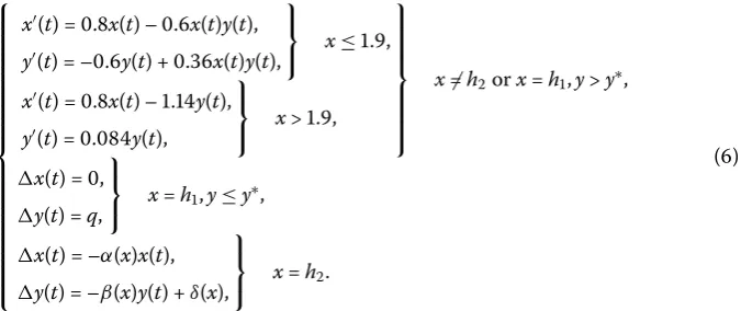
Based on the above works and the analysis, the state-dependent impulsive predator-prey system with Holling type-I functional response can be written as
⎧
where the density of the pest population and the natural enemy population are expressed byx(t) andy(t), respectively. The intrinsic growth rate of pest, the predation coefficient and the death rate of natural enemy are denoted bya,bandc, respectively. <r< means the conversion coefficient,qis the release amount of natural enemy at timeth, whileδis the release amount of natural enemy at timeth.a,b,r,c,d,q,h,h are all positive con-stants,y∗=ab,α,βrepresent the proportion of pests and natural enemies which are killed by pesticides, respectively. In this paper,α(x),β(x) andδ(x) are continuous functions
of system () is discussed by the successor function method and Bendixson theorem of impulsive differential equations. In Section , sufficient conditions for the stability of pe-riodic solutions of system () obtained by analogue of the Poincaré criterion are presented. In Section , it is shown that the conclusions are verified by numerical simulation, and the optimization problem is considered in order to minimize the total cost of pest control. Finally, a summary is made.
2 Preliminaries
At first, we consider the free system of system ()
⎧ ⎪ ⎪ ⎪ ⎪ ⎪ ⎪ ⎨ ⎪ ⎪ ⎪ ⎪ ⎪ ⎪ ⎩
x(t) =ax(t) –bx(t)y(t), y(t) = –cy(t) +rbx(t)y(t),
⎫ ⎬
⎭ x≤x,
x(t) =ax(t) –bxy(t), y(t) = –cy(t) +rbxy(t),
⎫ ⎬
⎭ x>x.
()
Define the following function:
(x,y) =
x x∗
–c+r(s) (s) ds+
y y∗
s–y∗ s ds.
It is easy to know that(x,y) is positive definite in the first quadrant and it satisfies all conditions of the Lyapunov function.
The derivative of(x,y) is
(x,y) = rxy
∗
(x)
(x) –x∗(x
∗)
x∗ – (x)
x
. ()
We can obtain that(x,y)≡ ifx≤x, then all solutions of system () constitute a set
{(x,y)|(x,y)≤(x,y∗)}, which is a closed orbit(x,y) =, where <<(x,y∗). If x>x, we have(x,y) > , then the orbit of system () always passes through the closed curve(x,y) =atx>xand out of the curve(x,y) =(x,y∗).
Thus, we observe the line
l(x,y) =y+x–m, m> ,x<x≤h,
wherehis a threshold of system (). The derivative ofl(x,y) is as follows:
l(x,y)|l==x+y=ax–bxy–cy+rbxy
=ax–bx(m–x) –c(m–x) +rbx(m–x)
= (ax+bx+c–rbx)x– (bx+c–rbx)m
≤(ax+bx+c–rbx)h– (bx+c–rbx)m.
Lemma .
(i) System()has two stable states:saddle pointO(, )and stable centerE(rbc,ab)when
x≤xand satisfiesx≥rbc.
(ii) The orbits of system()go across the linel= from the right to the left,which satisfiesx<x≤handm>(ax+bxbx++c–c–rbxrbx)h,and intersect the linex=x. Some basic definitions and lemmas are given as follows.
Definition .([]) Consider the general model with state-dependent impulse
⎧ ⎪ ⎪ ⎪ ⎪ ⎪ ⎪ ⎨ ⎪ ⎪ ⎪ ⎪ ⎪ ⎪ ⎩
x(t) =P(x,y), y(t) =Q(x,y),
⎫ ⎬
⎭ (x,y) /∈M{x,y},
x(t) =U(x,y), y(t) =V(x,y),
⎫ ⎬
⎭ (x,y)∈M{x,y},
()
whereM(x,y) is called an impulsive set, and letNbe the corresponding phase set.M(x,y) andN(x,y) represent the curve line or straight line on the plane. There exists a continuous impulse mappingI:I(M) =N. We define a dynamic system constituted by the definition of solution of state impulsive differential equation () as semi-continuous dynamic systems, which is denoted as ( ,f,I,M).
Definition .([]) Assume that the pulse setMand the phase setNare both straight lines, as shown in Figure . For any pointB∈N, then(B,t) =C∈M,I(C) =B+∈N, we denote the ordinates of pointsBandB+byy
BandyB+, respectively. ThenB+is defined as the successor point ofB, andf(B) =yB+–yBis the successor function of pointB.
Definition .([]) An orbit(Q,T) is called order- periodic solution with periodT if there exists a pointQ∈NandT> such thatQ=(Q,T)∈MandQ+=I(Q) =Q.
Definition .([]) For system (), the orbit starting from the pointAreaches the point AonLM, and then jumps onto the pointA+ onLN, that is, the orbit moves fromAtoA,
and then toA+. Similarly, the orbit moves fromBtoB, and then toB+. Thus the region k encircled by the closed curveABBA is an invariant set of system ().kis called the Bendixson region of system ().
Lemma .([]) The successor function defined in Definition.is continuous.
Lemma .([]) In system(),if there exist A∈N,B∈N satisfying the successor function f(A)f(B) < ,then there must exist a point Q(Q∈N)satisfying Q between the point A and the point B such that f(Q) = ,then system()has an order-periodic solution.
Lemma .([] Bendixson theorem of impulsive differential equations) Assume that k is a Bendixson region of system(),if k does not contain any critical points of system(), then system()has an order-periodic solution in k.
Lemma .([] Analogue of the Poincaré criterion) The T -periodic solution x=ξ(t),y=
is orbitally asymptotically stable if the multiplierμsatisfies the condition|μ|< ,where
μ=
In this paper, we assume that the conditionc≤rbxholds. Based on the biological sig-nificance of system (), we only considerD={(x,y)|x≥,y≥}.
3 Existence of order-1 periodic solution
In this section, the existence of order- periodic solution of system () is investigated by using the differential equation geometry theory and Bendixson theorem of impulsive dif-ferential equations. Here we denote
M=
Isoclinic lines of system () are denoted as follows:
L=
(x,y)y=a
b, ≤x≤x
,
L=
(x,y)x= c
rb, ≤x≤x,y≥
,
L=
(x,y)y= a bx
x,x>x,y≥a b
.
For convenience, the coordinate of any pointCis defined as (xc,yc). If the pointQ(h,yQ)∈
M, pulse occurs at the pointQ, the impulsive function transfers the pointQintoQ+∈N. By Lemma ., the orbit with any initiating point ofD={(x,y)|x≥,y≥}will intersect the setNorNwith time increasing; therefore, we consider the following cases.
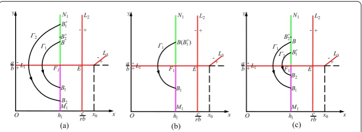
3.1 The orbit starting from the point ofN1
In this case, we havex≤x, <h<rbc <x. For convenience, we denote the intersection of LandLbyE(rbc,ab), and the pointF(h,ab) is the intersection ofLandN. The orbitof system () passes through the pointB(h,ab+ε)∈NaboveF, whereε> , and intersects with the pulse setMatB(h,yB). Then the orbit jumps back toNatB
+
(h,yB+q) from Mdue to the pulse action.
By regulatingq, the position ofB+ has the following three subcases. CaseIyB<yB+q.
In this case, the pointB+ is aboveB, thus the successor function ofBisf(B) =yB+q– (ab+ε) > . On the other hand, the orbitpassing through the pointB+ intersects with MatB(h,yB) because any two orbits are disjoint, then we haveyB<yB<
a
b. The point
Bis mapped toB+(h,yB+q) after impulsive effect. The pointB+is located aboveFand underB+
, thus the successor function ofB+ isf(B+) =yB +q– (yB+q) < . Therefore, f(B)f(B+) < .
From the above discussion, it is easy to know that the regionGencircled by the closed curveB+BBBis a positive invariant set of system () and it contains no equilibrium point. By Lemma ., there exists an order- periodic solution of system () (see Figure (a)).
CaseIIyB=yB+q.
In this case, the successor pointB+
is exactlyB, thenf(B) =yB+q– (
a
b+ε) = , thus the
curveBBB+ forms a periodic solution of system () (see Figure (b)).
CaseIIIyB>yB+q. In this case, the pointB+
is below the pointB, thus the successor function ofBisf(B) = yB+q– (
a
b+ε) < . On the other hand, the orbitpassing through the pointB
+
intersects withMatB(h,yB) because any two orbits are disjoint, then we haveyB<yB<
a b. The
pointBis mapped toB+(h,yB+q) after impulsive effect. The pointB +
is located aboveF and underB+
, then the successor function ofB+ isf(B+) =yB+q– (yB+q) > . Therefore, f(B)f(B+
) < . Thus there exists an order- periodic solution of system () by Lemma . (see Figure (c)).
Based on the above analysis, we get the following theorem.
Theorem . If x≤xand <h<rbc <x,there exists an order-periodic solution of system().
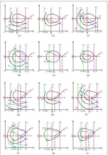
3.2 The orbit starting from the point ofN2
In this subsection, we assume the lineLintersects withL,NandMat pointsE(rbc,ab), B(( –α)h,ab) andF(h,ab), respectively. By Lemma . and qualitative analysis, there exists a unique closed orbitof system () which contains the pointEand tangents toM at the pointF. There is an orbitthat tangents toNat the pointBand intersectsM at the pointB(h,yB). The orbitjumps back toB+(( –α)h, ( –β)yB+δ)∈Nafter impulsive effect. By regulatingδ, if ( –α)h≤h, the case can be discussed like the case in Section .. And if ( –α)h>h, two cases should be discussed.
CaseI The orbitand the phase setNare disjoint andx≤x, <h< ( –α)h<rbc < h≤x. For this case, we have three subcases to be discussed.
CaseI(a)yB+q<yB.
If the pointB+ is below the pointB, we havef(B) =yB+–yB< . Then we choose another
orbit which is very close to thex axis and intersects withN at one point denoted byC(( –α)h,yC), then intersects withM at the pointB(h,yB). The orbitjumps back toB+
(( –α)h, ( –β)yB+δ)∈N after a pulse action, and it is aboveC, then the successor function of pointCisf(C) =yB+ –yC> . Therefore,f(B)f(C) < . According
to Lemma ., there must be Qwhich meetsyC<Q<yB in the phase set N to make
f(Q) =yQ+–yQ= , then there is an order- periodic solution of system () (see Figure (a)). CaseI(b)yB+q=yB.
In this subcase, the successor pointB+ is exactlyB, thenf(B) =yB+ –yB= , thus the
curveBBB+ forms a periodic solution of system () (see Figure (b)). CaseI(c)yB+q>yB.
If the pointB+
lies above the pointB, there isf(B) =yB+ –yB> . We select the orbit
which tangents toFand intersects withNandMatC(( –α)h,yC) andB(h,yB). The pointBis influenced by pulse toB+(h,yB+q)∈N. By the existence and uniqueness of impulsive differential equations, we haveyB <yB. Then we getf(C) =yB+ – (yC) < . Thus,f(B)f(B+
) < . According to Lemma ., there must beQwhich meetsyB<Q<yC
in the phase setNto makef(Q) =yQ+–yQ= , then there is an order- periodic solution of system () (see Figure (c)).
Figure 3 The orbit starting from the phase setN2(cases in Section 3.2). (a)Case I(a).(b)Case I(b).
(c)Case I(c).(d)Case II(a).(e)Case II(b).(f)Case II(c).(g)Case III(a).(h)Case III(b).(i)Case III(c).(j)Case IV(a).
(k)Case IV(b).(l)Case IV(c).
CaseII(a)yF+<yPoryF+>yP. In this subcase, the pointF+
is belowPor aboveP. By following similar analysis as that in Case I(a) or Case I(c), we can prove there exists an order- periodic solution of system () (see Figure (d)).
CaseII(b)yF+
In this subcase, the pointF+coincides withP orP, then we getf(P) =yF+–yP= or f(P) =yF+–yP = , thus an order- periodic solution of system () is existent (see Figure (e)).
CaseII(c)yP<yF+ <yP.
If the pointF+is betweenPandP, because any two trajectories are disjoint, then the orbit crosses the phase setNatF+
and does not intersect with the impulse setM, thus there is no order- periodic solution. According to the biological background, there are not a lot of pests in the farmland, crop damage is very small, therefore, it does not need pulse (see Figure (f )).
On the other hand, the lineL intersects withLandN at pointsE(rbc,ab) andB(( – α)h,ab), respectively, the lineLintersects withMatF(h,ah
bx). According to Lemma . and qualitative analysis, there exists a unique closed orbitof system () which contains the pointEand tangents toMat the pointF. There is an orbitthat tangents toNat the pointBand intersectsMat the pointB(h,yB). The orbitjumps back toB
+ (( – α)h, ( –β)yB+δ)∈Nafter impulsive effect. By regulatingδ, if ( –α)h≤h, the case can be discussed like the case in Section .. And if ( –α)h>h, we have two subcases to be discussed as follows.
CaseIII The orbitand the phase setNare disjoint andx>x, <h< ( –α)h<rbc ≤ x<h.
The method of proof is similar to Case I, here we omit it (see Figures (g), (h) and (i)). CaseIV The orbitcrosses the phase setNandx>x, <h< ( –α)h<rbc ≤x<h. The method of proof is similar to that in Case II, here we omit it (see Figures (j), (k) and (l)).
Moreover, ifx<x, <h< ( –α)h<h<rbc ≤x, the proof process is similar to that in Case I, there is no longer detailed description and graphic analysis.
From the above analysis, we get the following theorems.
Theorem .
() If the orbitand the phase setNare disjoint andx≤x,
<h< ( –α)h<rbc <h≤x,there exists an order-periodic solution of system(). () If the orbitcrosses the phase setNandx≤x, <h< ( –α)h<rbc <h≤x,
there are the following two conditions:
(i) whenyF+≥yPoryF+≤yP,an order-periodic solution of system()is existent; (ii) whenyP<yF+<yP,there is no order-periodic solution of system().
Theorem .
() If the orbitand the phase setNare disjoint andx>x,
<h< ( –α)h<rbc ≤x<h,there exists an order-periodic solution of system(). () If the orbitcrosses the phase setNandx>x, <h< ( –α)h<rbc ≤x<h,
there are the following two conditions:
(i) whenyF+≥yPoryF+≤yP,an order-periodic solution in system()is existent; (ii) whenyP<yF+<yP,there is no order-periodic solution of system().
4 Stability of order-1 periodic solution
In this section, under the existence condition of periodic solution of system (), we discuss its stability by Lemma ..
4.1 The orbit starting from the phase setN1
Letx=ξ(t),y=η(t) be aT-periodic solution of system () andξ=ξ(T),η=η(T);ξ=
Theorem . If c<rbx and a+bq–
periodic solution of system()is stable.
4.2 The orbit starting from the phase setN2
Let x=u(t),y=v(t) be a T-periodic solution of system () and u =u(T) =h,v =
The following theorem is obtained.
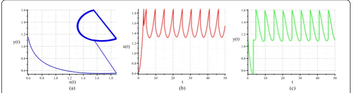
Figure 4 Numerical simulation of Example 1. (a)Phase portrait ofx(t) andy(t) onh1= 0.6.(b)Time series
ofx(t).(c)Time series ofy(t).
5 Numerical simulations and optimization 5.1 Numerical simulations
In this section, specific examples are given to verify the feasibility of the conclusions. Let a= .,b=c=r= .,x= .,h= .,αmax= .,βmax= .,δmax= .,δmin= ., then the equilibrium point of free system isE(., ). Inserting these parameter values into system (), we get
⎧ (c) show that system () has an order- periodic solution which is stable.
Example Leth= . and the initial value be (., .). By a direct calculation, we have α= .,β= . andδ= .. Figures (a), (b) and (c) show that system () has a stable order- periodic solution. By observing carefully from Figure (b), we can estimate that the period of order- periodic solution isT= ..
Example Whenh= , let the initial value be (, .), thenα= .,β= . andδ= .. Figures (a), (b) and (c) show that system () has an order- periodic solution with periodT= . which is stable.
Figure 5 Numerical simulation of Example 2. (a)Phase portrait ofx(t) andy(t) onh2= 1.88.(b)Time series
ofx(t).(c)Time series ofy(t).
Figure 6 Numerical simulation of Example 3. (a)Phase portrait ofx(t) andy(t) onh2= 5.(b)Time series of
x(t).(c)Time series ofy(t).
Figure 7 Numerical simulation of Example 4. (a)Phase portrait ofx(t) andy(t) onh2= 1.(b)Time series of
x(t).(c)Time series ofy(t).
stable order- periodic solution. By observing carefully from Figure (b), we can estimate that the period of order- periodic solution isT= ..
5.2 Determination and optimization of economic thresholdh2
The integrated control method of spraying pesticides and releasing natural enemies not only speeds up the death rate of pests, but also avoids the excessive damage to the crops; at the same time, the ecological balance is ensured. In order to ensure the best use of the material, the shortest time and the highest efficiency, the following optimal problem is investigated to find the best economic threshold.
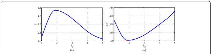
Figure 8 The change in the periodTand the cost per unit time F/T on the economic thresholdh2. (a)The change in the period T on the economic thresholdh2.(b)The cost per unit time F/T on the economic
thresholdh2.
of intensity of pesticide sprayingα(h), and the released amount of natural enemies are given byδ(h). Then we haveF(h) =dα(h) +dδ(h), and the optimization model is established as follows:
minF(h)
T(h)
s.t.h≤h≤h.
The objective function is solved to find out the best economic thresholdh∗, so as to obtain the optimal pesticide control intensityδ∗=δ(h∗), to find an optimal release amount of nat-ural enemiesα∗=α(h∗), and to find an optimal control period of pestT∗=T(h∗). Figure illustrates the variation of periodT and the cost per unit timeF/T with the economic thresholdh, whered=d= ,, i.e.,d/d= . From Figures (a) and (b), we can see that the optimal economic threshold ish∗= ., the optimal pesticide control intensity isα∗= ., the optimal release amount of natural enemy isδ∗= ., and the optimal control period of the pest isT∗= ..
6 Conclusion
In this paper, according to the different degrees of damage on crops, feedback control with two state dependent impulses is adopted on the pest management. When the den-sity of pests reaches the slightly harmful thresholdh, only the biological control method is adopted; when the density of pests reaches the economic thresholdh, the method of combining biological and chemical control is used, which can make the density of pests less than a given threshold and maintain the ecological balance. Analysis shows that this method is effective. Finally, numerical simulations are carried out to verify effectiveness of the control strategy. In addition, an optimization problem is proposed and solved, the optimal economic threshold is determined under the condition that the total cost is min-imum. However, there are some deviations in the results, which need to be improved.
Acknowledgements
The paper was supported by the National Natural Science Foundation of China (No. 11371230), Shandong Provincial Natural Science Foundation, China (No. ZR2015AQ001), SDUST Research Fund (2014TDJH102), and Joint Innovative Center for Safe and Effective Mining Technology and Equipment of Coal Resources, Shandong Province of China.
Competing interests
The authors declare that they have no competing interests.
Authors’ contributions
Author details
1College of Mathematics and Systems Science, Shandong University of Science and Technology, 579 Qianwangang Road, Qingdao, 266590, China. 2State Key Laboratory of Mining Disaster Prevention and Control Co-founded by Shandong Province and the Ministry of Science and Technology, Shandong University of Science and Technology, 579 Qianwangang Road, Qingdao, 266590, China. 3Department of Mathematics, University of Ruhuna, Matara, 81000, Sri Lanka.
Publisher’s Note
Springer Nature remains neutral with regard to jurisdictional claims in published maps and institutional affiliations.
Received: 15 May 2017 Accepted: 31 July 2017 References
1. Bai, Z, Zhang, S, Sun, S, Yin, C: Monotone iterative method for fractional differential equations. Electron. J. Differ. Equ.
2016(6), 1 (2016)
2. Wang, F, Liu, Z, Zhang, Y, Chen, CLP: Adaptive fuzzy control for a class of stochastic pure-feedback nonlinear systems with unknown hysteresis. IEEE Trans. Fuzzy Syst.24(1), 140-152 (2016)
3. Wang, F, Liu, Z, Zhang, Y, Chen, CLP: Adaptive quantized controller design via backstepping and stochastic small-gain approach. IEEE Trans. Fuzzy Syst.24(2), 330-343 (2016)
4. Meng, X, Zhao, S, Feng, T, Zhang, T: Dynamics of a novel nonlinear stochastic SIS epidemic model with double epidemic hypothesis. J. Math. Anal. Appl.433(1), 227-242 (2016)
5. Guo, S, Ma, W: Global behavior of delay differential equations model of HIV infection with apoptosis. Discrete Contin. Dyn. Syst., Ser. B21(1), 103-119 (2016)
6. Zhang, T, Meng, X, Zhang, T: Global analysis for a delayed SIV model with direct and environmental transmissions. J. Appl. Anal. Comput.6(2), 479-491 (2016)
7. Wang, W, Ma, W, Lai, X: Repulsion effect on superinfecting virions by infected cells for virus infection dynamic model with absorption effect and chemotaxis. Nonlinear Anal., Real World Appl.33, 253-283 (2017)
8. Wang, W, Ma, W, Lai, X: A diffusive virus infection dynamic model with nonlinear functional response, absorption effect and chemotaxis. Commun. Nonlinear Sci. Numer. Simul.42, 585-606 (2017)
9. Jiang, Z, Ma, W: Permanence of a delayed SIR epidemic model with general nonlinear incidence rate. Math. Methods Appl. Sci.38(3), 505-516 (2014)
10. Braverman, E, Chatzarakis, GE, Stavroulakis, IP: Iterative oscillation tests for differential equations with several non-monotone arguments. Adv. Differ. Equ.2016(1), 87 (2016)
11. Miao, A, Zhang, J, Zhang, T, Pradeep, BGSA: Threshold dynamics of a stochastic SIR model with vertical transmission and vaccination. Comput. Math. Methods Med.2017, 1-10 (2017)
12. Zhang, T, Zhang, T, Meng, X: Stability analysis of a chemostat model with maintenance energy. Appl. Math. Lett.68, 1-7 (2017)
13. Xu, X: A deformed reduced semi-discrete Kaup-Newell equation, the related integrable family and Darboux transformation. Appl. Math. Comput.251, 275-283 (2015)
14. Zhang, Y, Dong, H, Zhang, X, Yang, H: Rational solutions and lump solutions to the generalized-dimensional Shallow Water-like equation. Comput. Math. Appl.73(2), 246-252 (2017)
15. Wang, W, Ma, W: A diffusive HIV infection model with nonlocal delayed transmission. Appl. Math. Lett.75, 96-101 (2018)
16. Bainov, D, Simeonov, P: Impulsive Differential Equations: Periodic Solutions and Applications. Chapman & Hall/CRC, Boca Raton (1993)
17. Nieto, JJ, O’Regan, D: Variational approach to impulsive differential equations. Nonlinear Anal., Real World Appl.10(2), 680-690 (2009)
18. Ballinger, G, Liu, X: Permanence of population growth models with impulsive effects. Math. Comput. Model.26(12), 59-72 (1997)
19. Zhao, W, Li, J, Meng, X: Dynamical analysis of SIR epidemic model with nonlinear pulse vaccination and lifelong immunity. Discrete Dyn. Nat. Soc.2015, Article ID 848623 (2015)
20. Liu, B, Zhang, Y, Chen, L: Dynamic complexities of a Holling I predator-prey model concerning periodic biological and chemical control. Chaos Solitons Fractals22(1), 123-134 (2004)
21. Zhang, H, Jiao, J, Chen, L: Pest management through continuous and impulsive control strategies. Biosystems90(2), 350-361 (2007)
22. Meng, X, Zhang, L: Evolutionary dynamics in a Lotka-Volterra competition model with impulsive periodic disturbance. Math. Methods Appl. Sci.39(2), 177-188 (2016)
23. Zhang, T, Ma, W, Meng, X: Global dynamics of a delayed chemostat model with harvest by impulsive flocculant input. Adv. Differ. Equ.2017, 115 (2017)
24. Pang, G, Chen, L: Periodic solution of the system with impulsive state feedback control. Nonlinear Dyn.78(1), 743-753 (2014)
25. Li, Z, Wang, T, Chen, L: Periodic solution of a chemostat model with Beddington-DeAnglis uptake function and impulsive state feedback control. J. Theor. Biol.261(1), 23-32 (2009)
26. Zhao, Z, Wang, T, Chen, L: Dynamic analysis of a turbidostat model with the feedback control. Commun. Nonlinear Sci. Numer. Simul.15(4), 1028-1035 (2010)
27. Yang, J, Tang, G, Tang, S: Modelling the regulatory system of a chemostat model with a threshold window. Math. Comput. Simul.132, 220-235 (2017)
28. Jiang, G, Lu, Q: Impulsive state feedback control of a predator-prey model. J. Comput. Appl. Math.200(1), 193-207 (2007)
30. Liu, B, Tian, Y, Kang, B: Existence and attractiveness of order one periodic solution of a Holling II predator-prey model with state-dependent impulsive control. Int. J. Biomath.5(3) (2012)
31. Cheng, H, Zhang, T, Wang, F: Existence and attractiveness of order one periodic solution of a Holling I predator-prey model. Abstr. Appl. Anal.2012, Article ID 126018 (2012)
32. Tang, S, Tang, B, Wang, A, Xiao, Y: Holling II predator-prey impulsive semi-dynamic model with complex Poincar map. J. Differ. Equ.81(3), 1575-1596 (2015)
33. Zhang, T, Ma, W, Meng, X, Zhang, T: Periodic solution of a prey-predator model with nonlinear state feedback control. Appl. Math. Comput.266, 95-107 (2015)
34. Zhang, T, Zhang, J, Meng, X, Zhang, T: Geometric analysis of a pest management model with Holling’s type III functional response and nonlinear state feedback control. Nonlinear Dyn.84(3), 1529-1539 (2016)
35. Tian, Y, Zhang, T, Sun, K: Dynamics analysis of a pest management prey-predator model by means of interval state monitoring and control. Nonlinear Anal. Hybrid Syst.23, 122-141 (2017)
36. Zhang, H, Georgescu, P, Zhang, L: Periodic patterns and Pareto efficiency of state dependent impulsive controls regulating interactions between wild and transgenic mosquito populations. Commun. Nonlinear Sci. Numer. Simul.
31(1-3), 83-107 (2016)
37. Tian, Y, Sun, K, Chen, L: Modelling and qualitative analysis of a predator-prey system with state-dependent impulsive effects. Math. Comput. Simul.82(2), 318-331 (2011)
38. Cheng, H, Wang, F, Zhang, T: Multi-state dependent impulsive control for pest management. J. Appl. Math.2012, Article ID 381503 (2012)
39. Zhao, L, Chen, L, Zhang, Q: The geometrical analysis of a predator-prey model with two state impulses. Math. Biosci.
238(2), 55-64 (2012)
40. Tang, S, Tang, G, Cheke, RA: Optimum timing for integrated pest management: modelling rates of pesticide application and natural enemy releases. J. Theor. Biol.264(2), 623-638 (2010)
41. Liu, L, Meng, X: Optimal harvesting control and dynamics of two-species stochastic model with delays. Adv. Differ. Equ.2017(1), 18 (2017)
42. Sun, K, Zhang, T, Tian, Y: Theoretical study and control optimization of an integrated pest management predator-prey model with power growth rate. Math. Biosci.279, 13-26 (2016)
43. Sun, K, Zhang, T, Tian, Y: Dynamics analysis and control optimization of a pest management predator-prey model with an integrated control strategy. Appl. Math. Comput.292, 253-271 (2017)
44. Chen, L: Pest control and geometric theory of semi-continuous dynamical system. J. Beihua Univ. Nat. Sci.12(1), 1-12 (2011)