A machine learning framework for TCP round trip time estimation

(1)

R E S E A R C H

Open Access

A machine learning framework for TCP

round-trip time estimation

Bruno Astuto Arouche Nunes

1*

, Kerry Veenstra

1

, William Ballenthin

2

, Stephanie Lukin

3

and Katia Obraczka

1

Abstract

In this paper, we explore a novel approach to end-to-end round-trip time (RTT) estimation using a machine-learning technique known as theexperts framework. In our proposal, each of several ‘experts’ guesses a fixed value. The weighted average of these guesses estimates the RTT, with the weights updated after every RTT measurement based on the difference between the estimated and actual RTT.

Through extensive simulations, we show that the proposed machine-learning algorithm adapts very quickly to changes in the RTT. Our results show a considerable reduction in the number of retransmitted packets and an increase in goodput, especially in more heavily congested scenarios. We corroborate our results through ‘live’ experiments using an implementation of the proposed algorithm in the Linux kernel. These experiments confirm the higher RTT estimation accuracy of the machine learning approach which yields over 40% improvement when compared against both standard transmission control protocol (TCP) as well as the well known Eifel RTT estimator. To the best of our knowledge, our work is the first attempt to useon-line learning algorithmsto predict network

performance and, given the promising results reported here, creates the opportunity of applying on-line learning to estimate other important network variables.

1 Introduction

Latency is an important parameter when designing, man-aging, and evaluating computer networks, their protocols, and applications. One metric that is commonly used to capture network latency is the end-to-end round-trip time (RTT) which measures the time between data trans-mission and the receipt of a positive acknowledgment. Depending on how the RTT is measured (e.g., at which layer of the protocol stack), besides the time it takes for the data to be serviced by the network, the RTT also accounts for the ‘service time’ at the communication end points. In some cases, RTT measurement can be done implicitly by using existing messages; however, in several instances, explicit ‘probe’ messages have to be used. Such explicit measurement techniques can render the RTT estimation process quite expensive in terms of their communication and computational burden.

Several network applications and protocols use the RTT to estimate network load or congestion and therefore need

*Correspondence: [email protected]

1Department of Computer Engineering, Baskin School of Engineering, University of California, Santa Cruz, CA 95064, USA

Full list of author information is available at the end of the article

to measure it frequently. The transmission control proto-col, TCP, is one of the best known examples. TCP bases its error, flow, and congestion control functions on the estimated RTT instead of relying on feedback from the network. This pure end-to-end approach to network con-trol is consistent with the original design philosophy of the Internet which keeps only the bare minimum func-tionality in the network core, pushing everything else to the edges. Overlays such as content distribution networks (CDNs) (e.g., Akamai [1]) and peer-to-peer networks also make use of RTT as a ‘network proximity’ metric, e.g., to help decide where to re-direct client requests. There has also been increasing interest in network proximity infor-mation from applications that run on mobile devices (e.g., smart phones) in order to improve the user’s experience.

In this paper, we propose a novel RTT estimation technique that uses a machine-learning based approach called theexperts framework [2]. As described in detail in Section 3, the experts frameworkauses ‘on-line’ learn-ing, where the learning process happens intrials. At every trial, a number ofexpertscontribute to an overall predic-tion, which is compared to the actual value of the RTT (e.g., obtained by measurement). The algorithm uses the

(2)

prediction error to refine the weights of each expert’s con-tribution to the prediction; the updated weights are used in the next iteration of the algorithm. We contend that by employing the proposed prediction technique, network applications, and protocols that make use of the RTT do not have to measure it as frequently.

As an example application for the proposed RTT esti-mation approach, we use it to predict TCP’s RTT. Through extensive simulations and live experiments, we show that our machine learning technique can adapt to changes in the RTT faster and thus predict its value more accurately than the current exponential weighted moving average (EWMA) technique employed by most versions of TCP. As described in Section 2, TCP uses the RTT estimates to compute its retransmission time-out (RTO) timer [3], which is one of the main timers involved in TCP’s error and congestion control. When the RTO expires, the TCP sender considers the corresponding packet to be lost and therefore retransmits it. TCP relies on RTT predictions and measurements in order to set the RTO value properly. In TCP, the RTT is defined as the time interval between when a packet leaves the sender and until the reception, at the sender, of a positive acknowledgment for that packet.

If the RTO is too long, it can lead to long idle waits before the sender reacts to the presumably lost packet. On the other hand, if the RTO is set to be too aggressive (too short), it might expire too often leading to unnecessary retransmissions. Needless to say that setting the RTO is critical for TCP’s performance.

We can split the problem of setting TCP’s RTO into two parts. The first part is how to predict the RTT of the next packet to be transmitted, and the second is how the predicted RTT can be used to compute the RTO. In this paper, we focus on the first part of the problem, i.e., the prediction of the RTT; the second part of the problem, i.e., setting the RTO, is the focus of future work.

To estimate the RTT, we propose a new approach based on machine learning which will be described in detail in Section 3. Our experimental results show that RTT pre-dictions using the proposed technique are considerably more accurate when compared to TCP’s original RTT esti-mation algorithm and the well-known Eifel [4] timer. We then evaluate how this increased accuracy affects network performance. We do so by running network simulations as well as live experiments. For the latter, we have imple-mented both our machine learning as well as the Eifel mechanism in the Linux kernel.

The remainder of this paper is organized as follows. Section 2 presents related work, including a brief overview of TCP’s original RTT estimation technique. In Section 3, we describe our RTT prediction algorithm. Section 4 presents our experimental methodology, where we describe the scenarios conceived for our simulation studies, discuss simulation parameters, and define metrics

for performing evaluations. Sections 5 and 6, respec-tively, present our results from both simulation and live experiments. Finally, Section 7 concludes the paper and highlights directions for future work.

2 Related work

In this section, we present a brief overview of previous work on RTT estimation and later discuss some relevant machine learning applications.

2.1 TCP RTT estimation

TCP uses a time-out/retransmission mechanism to recover from lost segments. This time-out value needs to be greater than the current RTT to avoid unneces-sary retransmissions; on the other hand, if it is too high, it will cause TCP to wait too long to react to losses and congestion. In Jacobson’s well-known work [3], two state variables EstimatedRTT andRTTVAR keep the estimate of the next RTT measurement (SampleRTT) and the RTT variation, respectively.RTTVARis defined as an estimate of how much EstimatedRTT typically deviates fromSampleRTT. EstimatedRTTis updated according to an EWMA given by Equation 1, whereα = 1₈.RTTVARis calculated using Equation 2 which is also an EWMA; this time of the difference between SampleRTT and EstimatedRTT with gain β typically set to 1₄. Equation 3 sets the new value for theRTOas a function of EstimatedRTTandRTTVAR, whereKis usually 4.

EstimatedRTT=(1−α)·EstimatedRTT+α·SampleRTT (1)

RTTVAR=(1−β)·RTTVAR+β·|SampleRTT−EstimatedRTT| (2)

RTO=max(EstimatedRTT+K·RTTVAR, 2·ticks) (3)

Most current variants of TCP also implement Karn’s

Algorithm[5], which ignores theSampleRTTcorresponding

(3)

will become clear from the experimental results presented in Subsection 6.3, our approach is able to follow quite closely any abrupt changes in the RTT and outperforms both TCP’s original RTT estimator as well as that of Eifel’s. Another notable adaptive TCP RTT estimator was pro-posed in [7]. It uses the ratio of previous and current bandwidth to adjust the RTT. In [8], a TCP retrans-mission time-out algorithm based on recursive weighted median filtering is proposed. Their simulation results show that for Internet traffic with heavy tailed statistics, their method yields tighter RTT bounds than TCP’s origi-nal RTT computation algorithm. Leung et al. present work that focuses on changing RTO computation and retrans-mission polices, rather than improving RTT predictions [9].

2.2 Selected machine learning applications

Machine learning has been used in a number of other applications. Helmbold et al. use an experts framework algorithm to predict hard-disk drive’s idle time and decide when to attempt to save energy by spinning down the disk [10]. For this problem, the cost of making a bad decision (i.e., when spinning the disk down and back up costs more than simply leaving it on) is very well defined since the decision of spinning down the disk does not affect the length of the next idle time.

Unlike the spin-down example, when predicting the RTT, every prediction causes the next RTT to be set to a different value and that influences every event that hap-pens thereafter. Thus, the problem of defining the cost of a bad RTT prediction is not as straightforward. Our solution to this problem is discussed in Section 3.

Moreover, in the spin-down cost problem, the traces used in the evaluation were ‘off-line’ traces, i.e., traces cap-tured from live runs and later on used as input to the algorithms being evaluated. In the case of the spin-down problem, there is no problem in using off-line traces since the algorithm’s estimations do not influence the outcome of the next measurement. In the case of TCP RTT esti-mation, however, as previously discussed, since the RTT estimations influence TCP timers and these timers affect the outcome of the next RTT measurement, off-line traces can be used to set and tune parameters of the algorithm, but they are not suitable for evaluating the performance of the system. The work presented in [8,9,11,12] on RTT estimation compares their solution against TCP’s original RTT estimation algorithm, but they base their evaluation on off-line traces.

Machine learning techniques have not been commonly employed to address network performance issues. The work described in [13] is a notable exception and proposes the use of the stochastic estimator learning algorithm (SELA) to address the call admission control (CAC) prob-lem in the context of asynchronous transfer mode (ATM)

networks. Their goal was to predict in ‘real time’ if a call request should be accepted or not for various types of traffic sources. Simulation results show the statistical gain exhibited by the proposed approach compared to other CAC schemes. Another SELA-based approach, this time, applied to QoS routing in hierarchical ATM networks was proposed in [14]. In this approach, learning algorithms operating at various network switches determine how the traffic should be routed based on current network con-ditions. In the context of WiMax networks, a cross-layer design approach between the transport and physical lay-ers for TCP throughput adaptation was introduced in [15]. The proposed approach uses adaptive coding and modulation (ACM) schemes.

Mirza et al. propose a throughput estimation tool based on support vector regression modeling [16]. It predicts throughput based on multiple real-value input features. However, to the best of our knowledge, to date, no attempt to use on-line learning algorithms to predict network conditions has been reported.

3 Proposed approach

In this section, we present thefixed-share experts algo-rithm as a generic solution for on-line prediction. Later, we describe its application to the problem of predicting the RTT of a TCP connection.

3.1 The fixed-share experts algorithm

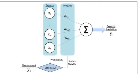
Our RTT prediction algorithm is based on the fixed-share experts algorithm [2] which uses ‘on-line learning’ based on the predictions of a set of fixedexpertsdenoted by{x1,. . .,xN}. In on-line learning, the learning process happens in trials. Figure 1 illustrates these trials and the algorithm itself. Under the fixed-share experts algorithm, at every trial t, the algorithm receives the predictions

xi∀i∈ {1,. . .,N}from a total ofNexperts and uses them to output a master predictionyˆt. After trialtis completed, the ‘ground truth’ valueytbecomes known and is used to compute the estimation error based on aloss function,L. The estimation error computed at trialtfor every expert

iis thus given byLi,t(xi,yt)which is used to update a set

of weights. The next prediction for trial t+ 1 is

calcu-lated using this new set of weights denoted byWt+1,i =

{wt+1,1,. . .,wt+1,i,. . .,wt+1,N}.

(4)

Figure 1Graphical representation of the general fixed-share experts algorithm for RTT estimation.

After updating the weights, the algorithm also ‘shares’ some of the weight of each expert among other experts. Thus, an expert who is performing poorly and had its weight severely compromised can quickly regain influ-ence in the master prediction once it starts predicting well again. The amount of sharing can be changed by using theαparameter, called thesharing rate. This allows the algorithm to adapt to ‘bursty’ behavior. Indeed, in Section 5, we use, among others, bursty traffic scenarios to evaluate the performance of our algorithm.

Algorithm 1 summarizes the steps involved in our fixed-share experts algorithm. The first line in the algorithm summarizes the algorithm’s parameters, namely: (1) the learning rateη, which we define as a positive real num-ber, and (2) the sharing rate α, a real number between zero and one that dictates the percentage of the weights shared at every trial. In our approach, expert weights are initialized uniformly, which is what is described in the ‘Initialization’ step of Algorithm 1. The basic four steps of our fixed-share experts algorithm are also summarized in Algorithm 1 (and in Figure 1). In step 1, the predic-tion defined as a the weighted average over the individual predictions xi of everyith expert is computed. The loss function is computed in step 2 and is used in step 3 to penalize and decrease the weights of the experts that are not performing well, and in step 4, experts share their weight based on the sharing rateα.

In [2], the basic version of the experts framework is presented along with bounds for different loss functions. The algorithm is also analyzed for different prediction

functions, including the weighted averaging we use. The implementation described in this paper, with the interme-diatepoolvariable, costsO(1)time per expert per trial.

3.2 Applying experts to TCP’s RTT prediction

To apply the proposed algorithm to TCP’s RTT-prediction problem, the experts predictionsxishown in Algorithm 1 serve as predictions for the next RTT measured. yt is the RTT value at the present trial, equivalent to the Sam-pleRTTin the original TCP RTT estimator.yˆ_tis the output of the algorithm, or in other words, the RTT prediction itself, equivalent to theEstimatedRTTin the original TCP RTT predictor, mentioned in Section 2.

Algorithm 1 Fixed-share experts algorithm Parameters:η >0 and 0≤α≤1

Initialization:w1,1=. . .=w1,N = _N1 1) Prediction:

ˆ

yt=

N

i=1wt,i·xi N

i=1wt,i

2) Computing the loss:∀i: 1,. . .,N

Li,t(xi,yt)=

(xi−yt)2 ,xi≥yt

2·yt ,xi<yt 3) Exponential updates:∀i: 1,. . .,N

w_t,i=wt,i·e−ηLi,t(yt,xi)

4) Sharing weights:∀i: 1,. . .,N

pool=N_i₌₁α·w_t,i

(5)

We want the loss functionLi,t(xi,yt)to reflect the real cost of making wrong predictions. In our implementation (see Algorithm 1), the loss function has different penalties for overshooting and undershooting the RTT estimate as they have different impact on the system’s behavior and performance. An underestimate of the RTT will result in an RTO computation that is less than the next measured RTT, causing unnecessary timeouts and retransmissions. We thus employ the following policies: if the measured RTTyt is higher than the expert’s prediction xi, then it means that this expert is contributing to a spurious time-out and should be penalized more than other experts that overshoot within a given threshold. Big over-shooters are more severely penalized. The challenge here is identify-ing the appropriate cost for miss-predictidentify-ing the RTT. The cost could be simply the difference between prediction and measurement, or a factor thereof. Exploring other loss functions for the TCP RTT estimation problem is the subject of future work.

Setting the valuexiof the experts is referred to as setting

the experts spacing. To space the experts is to

deter-mine the experts’ values and their distribution within the prediction domain. When predicting RTTs, the experts should be spaced betweenRTTmin and RTTmax, defined in some TCP implementations (including the one in the net-work simulator we used in our experimental evaluation) to be 1 and 128 ticks, respectively. Based on observations of several RTT datasets, we concluded that the majority of the RTT measurements are concentrated in the lower part of this interval. For that reason, we found that spacing the experts exponentially in that interval, instead of uniformly (or linearly), leads to better predictions. The exponential function used in our implementation of the Fixed-Share Experts approach isxi = RTTmin+RTTmax ·2

(i−N)

4 . The 1 4 multiplicative factor in the exponent of the spacing func-tion was experimentally chosen to smooth out its growth. This increases the difference between the experts and gen-erates diversity among them, which increases predictions’ granularity and accuracy.

Another consideration is that the algorithm, as stated in Algorithm 1, will continually reduce the experts’ weights towards zero. Thus, in order to avoid underflow issues in our implementation, we periodically rescale the weights. Different versions of the multiplicative weight algorithmic family, including amixing past approach that also mixes weights from past trials are discussed in [17]. However, the mixing past approach incurs higher space and time costs and thus was not considered in our work. Another sharing scheme known as variable-sharing was also con-sidered in preliminary experiments, where the amount of shared weights to each expert was dependent of their indi-vidual losses. However, the additional complexity and cost of this scheme outweighed its benefits in terms of RTT estimation accuracy.

4 Experimental methodology

We conduct simulations using the QualNet [18] network simulation platform. In all experiments, unless stated oth-erwise, the simulation area is 1,500 m×1,000 m and the simulated time is 25 min. The routing protocol used was AODV [19], and the medium access and physical layers defined at the IEEE 802.11.b [20] standard was used. The transmission radius was set to 100 m for all the nodes, which are initially placed in the simulation area uniformly distributed. On mobile scenarios, nodes move according to the random way point (RWP) mobility regime with 0 s of pause time and speed ranging between [1, 50] m/s. All nodes run file transmission protocol (FTP) applications to generate the TCP flows; TCP buffer size is the default TCP buffer size set to 16,384 bytes, and packet size is fixed at 512 bytes. For the reader convenience, we summarize the simulation parameters for all simulation scenarios in Table 1. The valuenais attributed to a given parameter in this table when it isnot applicable. These and other simu-lation parameters, such as traffic patterns and number of flows will be discussed further in the following sections in a per-scenario basis.

In Section 5, we present results for a total of five simu-lation scenarios, which are summarized, along with their parameters, in Table 1. The goal of having a variety of scenarios is to subject the proposed RTT estimation approach to a wide range of network conditions. Scenar-ios I and II representad hocmobile networks composed of 20 and 10 nodes, respectively. These two scenarios differ from each other only in terms of node density. Sce-nario III is a static wireless network composed of 20 nodes uniformly distributed over the simulated network area. Scenario IV is also a 20-node mobile network, but the traf-fic pattern is different from scenarios I and II. In scenario IV, we also vary the mobility of the network by varying the nodes’ average speed. Finally, scenario V is a wired network composed of eight nodes, four on each side of a bottleneck link.

It is important to highlight that the mobile scenarios employed in our evaluation were used to evaluate the pro-posed RTT estimation technique under conditions that cause high variability and randomness in the network and thus in the RTT values. Following the RWP mobil-ity regime, nodes move randomly causing data paths to break and new ones to be created which then results in high variability of the RTT. Our goal was then to ensure that our RTT estimator is able to adjust to high variability conditions and yield accurate RTT estimates.

We present our results in Section 5 using a number of performance metrics defined as follows:

• Mean error on RTT prediction: absolute difference between the RTT predictionyˆtand the measured

(6)

Table 1 Simulation parameters for each simulation scenario

Parameter Scenario I Scenario II Scenario III Scenario IV Scenario V

Routing AODV AODV AODV AODV fixed

Mobility RWP RWP none RWP na

MAC/PHY 802.11.b 802.11.b 802.11.b 802.11.b 802.3

Speed [min,max](m/s) [1,50] [1,50] 0 [1,10], [20,30], [40,50] na

Pause (sec) 0 0 0 0 na

Area (meters×meters) 1,500×1,000 1,500×1,000 1,500×1,000 1,500×1,000 na

Duration (min) 25 25 25 90 90

Number of nodes 20 10 20 20 8

1 T

T

t=1|ˆyt−yt|. In the simulations, RTT is

measured in ‘ticks’ of 500 ms. This value is equal to 4 ms in the real live experiments described in Section 6. The mean RTT prediction error metric is thus, also given in ‘ticks’.

• Average congestion window size (cwnd) : the size in bytes of the congestion window at the TCP sender, averaged over all prediction trials, defined as:

1 T

T

t=1cwndt, wherecwndtis the congestion

window size measured at trialt.

• Delivery ratio: ratio between total data packets received by the destination and data packets sent at the source, computed for every flow and averaged over all flows.

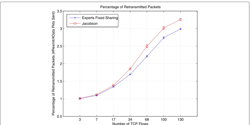
• Percentage of retransmitted packets: ratio between retransmitted data packets and total data packets sent at every flow, averaged over all flows.

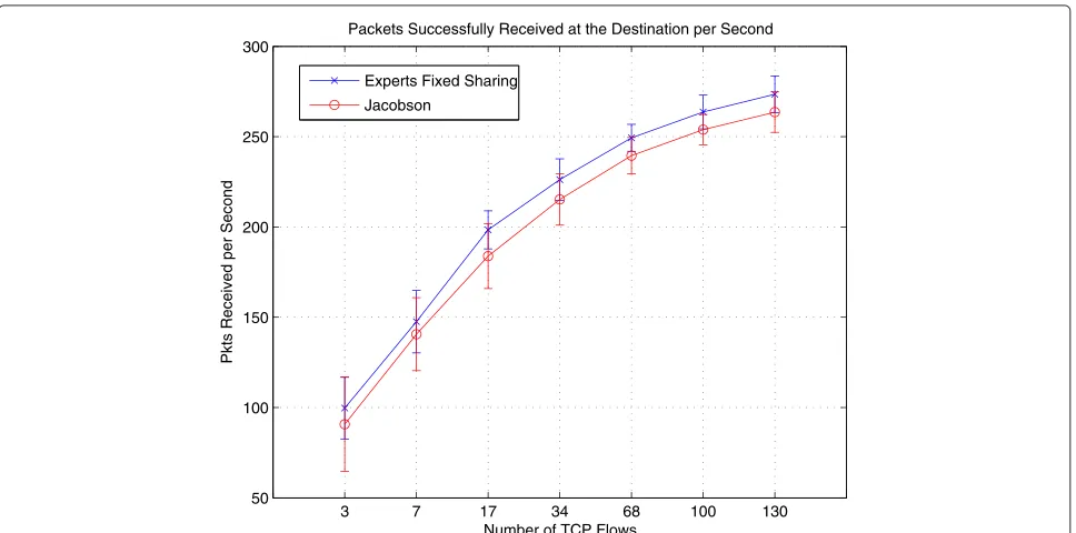
• Goodput: total number of useful (data) packets received at the application layer divided by the total duration of the flow and averaged for every flow, giving a ratio of packets per second.

Following, we discuss the impact of the parameters in the accuracy of the proposed RTT prediction algorithm and justify the choice of values set to these parameters in our simulation evaluations.

4.1 Impact of experts framework parameters (N,η,α) We experimented with several combinations of the fixed-share algorithm parameters. The number N of experts affects the granularity over the range of values the RTT can assume. In our experiments,N > 100 had no major impact on the prediction accuracy.

The learning rate η is responsible for how fast the experts are penalized for a given loss. We want to avoid values ofη that are too low since it increases the algo-rithm’s convergence time; conversely, if ηis too high, it forces the expert’s weights toward zero too quickly. If this is the case, then as weight rescaling kicks in, the algorithm assigns similar weights to all experts, making the algo-rithm’s master prediction fluctuate undesirably around

the mean value of the experts’ guesses. We chose a learn-ing rate in the interval 1.7< η <2.5 as it provides good prediction results for all the scenarios tested.

When sharing is not enabled, i.e.,α = 0, the outcome of the algorithm is given only by decreasing exponen-tial updates, making it harder for the algorithm to follow abrupt changes in the RTT measurements: experts that experience prolonged poor performance lack influence because their weights have become too depreciated. In this case, it would take more trials so that these experts start gaining greater importance in the master prediction. Enabling full sharing (α=1), similar weights are assigned to every expert, and the master prediction fluctuates close to a mean value among the experts guesses.

We present in more detail the simulation scenarios in the next section, highlighting the goals for every evalua-tion and discussing obtained results. Following our obser-vations, in all results reported hereafter concerning our proposed approach, we useN=100,η=2 andα=0.08.

5 Simulation results

In this section, we discuss simulation results obtained by applying the fixed-share experts framework to estimate TCP’s RTT and help set TCP’s RTO timer. We com-pare our results against TCP’s original RTT and RTO computation algorithm by Jacobson [3]. We evaluate the RTT prediction quality and how it impacts the previously defined performance metrics. We consider different sce-narios by varying network density, mobility, and traffic load. Both wireless as well as wired networks are used in our evaluation.

In all graphs presented below, each data point is com-puted as the average over 24 simulation runs with a confidence level of 90%.

5.1 Scenario I - mobile scenario (20 nodes)

(7)

to RTT fluctuations. For that reason, we also varied the number of TCP flows during the simulations to change network load and congestion levels. We evaluated scenar-ios with number of concurrent flows equal to 3, 7, 17, 34, 68, 100, and 130. Although flows were evenly distributed among nodes, they started at random times during the experiments and their sizes varied from 1,000 to 100,000 packets.

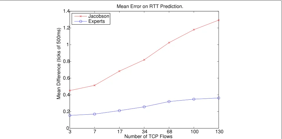
Figure 2 shows the mean differences between the pre-dictions of the experts framework and Jacobson’s algo-rithms when compared to the real RTT measurements. We observe that the experts framework improves RTT estimation accuracy considerably as the load in the net-work increases. This leads to more accurate setting of the RTO timer, which, in turn, reduces the relative number of packets retransmitted significantly, especially under heavy traffic conditions. As shown in Figure 3, retransmissions are reduced substantially (by as much as over 30%) with-out decreasing the number of packets sent. Note also the improvement in the goodput, i.e., total number of packets received (Figure 4).

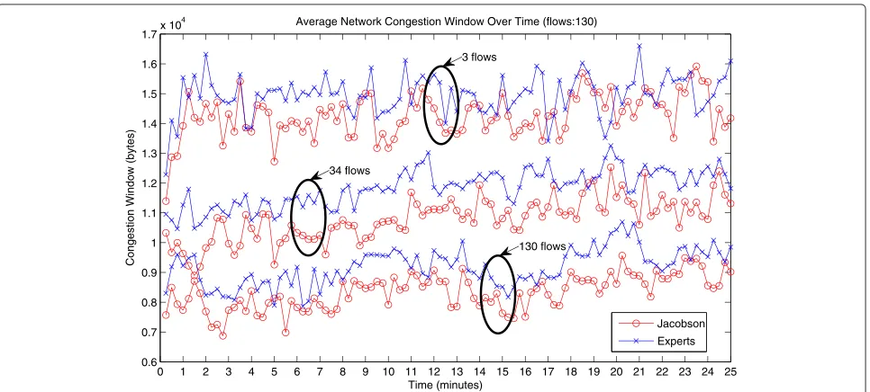
Our use of the experts framework not only improved the RTT predictions, thereby avoiding unnecessary retrans-missions, but also avoided unnecessary triggering of congestion-control mechanisms. Consequently, TCP’s congestion window (cwnd) is higher on average; this behavior is shown in Figure 5, which plots the average cwnd for the experts framework and Jacobson’s algo-rithms over the duration of the whole simulation for different congestion scenarios, i.e., different number of TCP flows. We can observe how the gap between the two

approaches increases with increasing congestion condi-tions. This indicates that the experts framework is able to better shield TCP’s congestion control from wide RTT fluctuations.

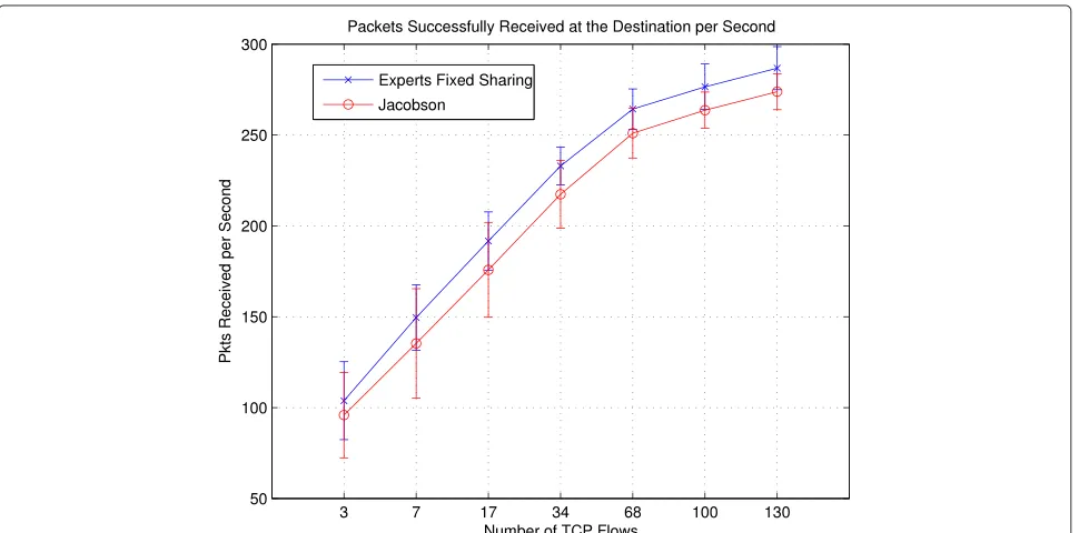
Figure 6 plots the average cwnd over the whole simula-tion time for 3, 34, and 130 flows. Each point in this plot is the mean cwnd over 24 simulation runs considering all nodes averaged over a 20-s time window. These plots cor-roborate the results shown in Figure 5, i.e., that the experts framework yields, on average, higher cwnd. We observe from Figures 7 and 4 that the proposed experts framework is also able to improve both the delivery ratio and goodput, which we define here as the absolute number of packets successfully delivered at the destination over the course of the simulation.

5.2 Scenario II - mobile scenario (10 nodes)

In this scenario, we try to subject the network to vary-ing network conditions in order to produce higher RTT variations. We accomplish that by running the same sce-nario, but now decreasing the density of the network, which includes only ten mobile nodes. The objective is to cause more frequent route changes which would result in more frequent and wider RTT variations. For exam-ple, in scenario I, the mean RTT variance for 34 and 100 flows are 0.4763 and 0.5501 ticks, respectively. For sce-nario II, with only ten nodes, the mean RTT variance for the same congestion scenarios are 0.7878 and 0.9315 ticks, respectively. Except for the reduced number of nodes, all the other parameters for this scenario are the same as before.

(8)

Figure 3Number of retransmitted packets in relation to the total number of packets transmitted on a 20-node MANET.

In Figure 8, we can compare the accuracy of the predic-tions for both algorithms. Similar to the previous scenario, as congestion increases with the number of flows, so does the variability of the RTT measurements, also increasing the mean error in the prediction. For the same num-ber of flows, we observe how the mean error increases from scenario I (Figure 2) to scenario II (Figure 8) due to the increase in the variation of the RTT. Network

performance metrics, such as number of retransmitted packets (Figure 9) and delivery ratio (Figure 10) exhibit trends similar to scenario I. Similar behavior is also observed for cwnd (Figure 11), delivery ratio (Figure 10), ratio of packets retransmitted (Figure 9), and goodput in (Figure 12). As in scenario I, we also observe that, as traf-fic load increases, the difference between the algorithms also increases for all the metrics.

(9)

Figure 5TCP’s cwnd for a 20-node MANET for different traffic loads.

5.3 Scenario III - stationary network

Our goal in this experiment is to isolate the effect of traffic load on the performance of the proposed RTT estima-tor. Therefore, we factor out node mobility and consider a wirelessad hocnetwork where all nodes are stationary. We varied traffic load the same way we did for scenario I.

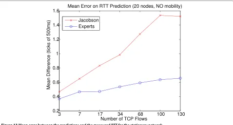
Figure 13 shows the accuracy of the prediction algo-rithms. Like in previous scenarios, increasing traffic load degrades the performance of the algorithms, although this

degradation is much more pronounced for Jacobson’s RTT predictor. This figure shows that the error of the original TCP RTT predictor can get up to around 130% larger than when using our proposed machine learning approach. For example, in Figure 13, we report an average error of 0.63 ticks for the experts framework, against 1.54 ticks for the original TCP estimator.

Moreover, when comparing the accuracy results for the stationary scenario with the mobile scenario with 20

0 1 2 3 4 5 6 7 8 9 10 11 12 13 14 15 16 17 18 19 20 21 22 23 24 25 0.6

0.7 0.8 0.9 1 1.1 1.2 1.3 1.4 1.5 1.6 1.7x 10

4

Time (minutes)

Congestion Window (bytes)

Average Network Congestion Window Over Time (flows:130)

Jacobson Experts 3 flows

34 flows

130 flows

(10)

3 7 17 34 68 100 130 0.976

0.978 0.98 0.982 0.984 0.986 0.988 0.99 0.992 0.994

Number of TCP Flows

Delivery Ratio

Delivary Ratio

Experts Fixed Sharing Jacobson

Figure 7Packet delivery ratio in a 20-node MANET.

nodes (Figure 2), it is possible to notice that the stationary scenario exhibits higher average estimation error for both algorithms. Figure 14 shows the average queue length in bytes for both mobile and stationary scenarios, for differ-ent number of flows. We observe that the average queue length for the mobile scenario is much lower. This can be explained by the fact that, in the static scenario, since routes between source and destination are less volatile,

queues build up as the traffic load increases and result in larger RTT fluctuations. This is especially the case of nodes that are carrying traffic that belong to multiple flows.

In the stationary scenario, the number of retransmit-ted packets is lower when using the proposed experts framework approach when compared against the number of retransmissions resulting from Jacobson’s algorithm, as we can see in Figure 15. When compared to the mobile

3 7 17 34 68 100 130

0 0.2 0.4 0.6 0.8 1 1.2 1.4 1.6 1.8 2

Number of TCP Flows

Mean Difference (ticks of 500ms)

Mean Error on RTT Prediction.

Jacobson Experts FW

(11)

3 7 17 34 68 100 130 0.5

1 1.5 2 2.5 3 3.5

Number of TCP Flows

Percentage of Retransmitted Packets (#Rexmit/#Data Pkts Sent)

Percentage of Retransmitted Packets

Experts Fixed Sharing

Jacobson

Figure 9Number of retransmitted packets in relation to the total number of packets transmitted for a 10-node MANET.

scenario, the number of retransmissions is lower for both algorithms since, in the stationary scenario, there are fewer losses due to route failure. Figure 16 shows the average cwnd size for different congestion levels. Once again, it is possible to see improvement in this metric when applying our proposed approach. However, with the increase in the RTT fluctuations in this scenario, as men-tioned before, the occurrence of spurious timeouts may

also occur. Thus, we experienced in this scenario a higher variability of the cwnd as seen by the larger confidence interval exhibited when comparing it to the cwnd results in Scenario I (Figure 5).

5.4 Scenario IV - bursty traffic

In this scenario, we subject the network to bursty traffic loads as a way to evaluate the performance of the proposed

3 7 17 34 68 100 130

0.974 0.976 0.978 0.98 0.982 0.984 0.986 0.988 0.99 0.992 0.994

Number of TCP Flows

Delivery Ratio

Delivary Ratio

Jacobson

(12)

3 7 17 34 68 100 130 0.7

0.8 0.9 1 1.1 1.2 1.3 1.4 1.5x 10

4

Number of TCP Flows

cwnd (bytes)

Congestions Window Size

Jacobson

Figure 11TCP cwnd for a 10-node MANET with different traffic loads.

RTT estimation strategy as traffic load fluctuates. The results shown here reflect the simulation of a network with 20 mobile nodes in which every node starts a TCP flow of 1,000 packets every 200 s; this happens through-out the 90 min of simulation. Thus, nodes would transmit for a while and then remain silent until the next cycle of 200 s. We also vary the speed of the nodes between (1, 10),

(20, 30), and (40, 50) m/s, which allows average speeds of 5, 25, and 45 m/s, respectively.

In relation to previous scenarios, the experts framework yields higher performance improvement when compared to Jacobson’s algorithm due to the fact that it is able to adapt to RTT fluctuations faster. This is attributed to the weight sharing feature of the experts. This performance

3 7 17 34 68 100 130

50 100 150 200 250 300

Number of TCP Flows

Pkts Received per Second

Packets Successfully Received at the Destination per Second

Jacobson

(13)

Figure 13Mean error between the predictions and the measured RTT for the stationary network.

improvement becomes evident when looking at the plot of the mean absolute error in Figure 17. In this figure, the difference between the algorithms prediction errors can vary from 100% for 25 m/s average speed, up to 200% for 5 m/s average speed. We can also observe that the impact of different levels of mobility are also different for both algorithms. While Jacobson’s RTT predictor appears to present strong variation with the mobility level, the proposed experts algorithm presents little variation when

changing the speed of the nodes. This behavior can be also explained by the fact that the experts framework is able to adapt quickly to abrupt RTT variations because of the sharing mechanism. The moving average applied in Jacobson’s algorithm, on the other hand, is not able to respond as fast.

Since the measured RTT fluctuations for this scenario are much greater, the mean prediction error in this case is larger than in the previous scenarios. We also report

(14)

Figure 15The number of retransmitted packets in relation to the total number of packets transmitted for both algorithms for the stationary scenario.

for this scenario a much lower number of retransmit-ted packets (Figure 18). It is also possible to observe an improvement in the other performance parameters, i.e., TCP’s cwnd, yielding higher goodput (Figure 19) when using our experts framework approach. Finally, Figure 20 shows the improvement in delivery ratio for this scenario.

It is also worth noting the interesting behavior present in the plots for all the reported network performance met-rics, where for lower speeds, these metrics reflect better network performance (i.e., lower number of retransmitted packets, higher goodput and higher delivery ratio), since the routing paths do not change as frequently. This incur

3 7 17 34 68 100 130

0.8 0.9 1 1.1 1.2 1.3 1.4 1.5 1.6 1.7 1.8x 10

4

Number of TCP Flows

cwnd (bytes)

Congestions Window Size

(15)

5 25 45 0.5

1 1.5 2 2.5 3

Average speed (m/s)

Jacobson Experts FW

Figure 17Mean absolute error between predicted and measured RTT for different node speeds in bursty traffic scenario.

in fewer losses and lower routing overhead. For the aver-age speed of 25 m/s, the situation changes and the metrics reflect the worst performance. However, when further increasing the average speed to 45 m/s, the network met-rics start to improve again. This behavior is consistent with the results presented in [21], which shows that, when topology changes happen at packet delivery time scales,

network capacity can improve when nodes are mobile rather than stationary.

5.5 Scenario V - wired network

Here, we simulate an eight-node wired network whose topology can be seen in Figure 21. In this scenario, we vary the traffic load by using 30, 70, and 100 concurrent

5 25 45

3 3.5 4 4.5 5 5.5 6

Average speed (m/s) Percentage of Retransmitted Packets

(16)

5 25 45 1.1

1.15 1.2 1.25 1.3 1.35x 10

6

Average speed (m/s)

Packets Successfully Received at the Destination per Second

Experts Jacobson

Figure 19Goodput for different node mean speeds in the bursty traffic scenario.

flows. Flows were evenly distributed among nodes but start at random times throughout the 90-min duration of the simulation. The size of a flow is uniformly distributed between 1,000 and 10,0000 packets.

As shown in Figure 22, the mean prediction error for Jacobson’s algorithm is almost four times higher than when using the experts framework. The benefits of the more accurate RTT estimates yielded by our approach is

illustrated in Figures 23,24,25 which show lower number of retransmitted packets, higher delivery ratio, and higher goodput as the number of TCP flows increases.

6 Linux implementation and experiments

In this section, we present our implementation of the fixed-share experts algorithm for the Linux kernel and report on the experiments we conducted and their results.

5 25 45

0.95 0.955 0.96 0.965 0.97 0.975 0.98

Delivery Ratio

Average speed (m/s) Delivary Ratio

(17)

1

2

3

4

5

6

7

8

Figure 21Simulated network topology for the wired scenario.

6.1 Fixed-point arithmetic

The simulation results reported in Section 5 refer to the implementation of the fixed-share experts algorithm (as described in Section 3) as implemented on the Qual-Net network simulator. This implementation uses real numbers. Thus, a straightforward Linux implementation would use floating point arithmetic [22] along with float-ing point functions of thegcccompiler’slibclibrary [23].

Unfortunately, while floating point numbers support both a wide range of values and high precision, the Linux oper-ating system lacks support for flooper-ating point manipulation in the kerneld.

An alternative is to usefixed pointarithmetic in which the location of the radix point within a string of digits is predetermined [24]. In our implementation, we define a fixed point arithmetic type with a 16-bit integral part and a 16-bit fractional part as shown below.

s b31· · ·b16 . b15· · ·b0

In our Linux implementation we used a sign magnitude representation in which a 33rd bit records the sign (an alternate implementation of the data type would reduce the integer part to 15 bits so that the resulting type would fit entirely within a single 32-bit processor register.)

Our fixed point numeric type has the following char-acteristics: range = −65535.99998to+65535.99998 and

precision = 0.000015. We consider these characteristics

adequate for the range of numeric values expected.

6.2 Linux implementation

We implemented both the fixed share experts algo-rithm and the Eifel algoalgo-rithm [4] in the Linux kernel version 2.6.28.3. We modified the function tcp_rtt_estimator() to return the output of the RTT as evaluated by either of the RTT prediction algo-rithms. Our implementation of the Eifel algorithm, to the best of our knowledge, is faithful to the algorithm described in [4] for predicting the RTT and setting the RTO.

Our Linux implementation of the fixed share experts algorithm differs from our QualNet implementation of the algorithm in two areas. First, the implementation scales RTT measurements. A measured RTT of 1 tick in the sim-ulator means 500 ms, while a measured RTT of 1 tick in the Linux implementation means 4 ms. Consequently, our Linux implementation scales RTT measurements from the operating system by ₁₂₅1 before passing them to the fixed share experts algorithm, and it scales RTT predic-tions from the experts algorithm by 125 before returning

30 70 100

1 2 3 4 5 6 7

Number of TCP Flows

Jacobson Experts FW

(18)

30 70 100 3

4 5 6 7 8 9 10 11 12

Number of TCP Flows

Jacobson

Figure 23Number of retransmitted packets in relation to the total number of packets transmitted for the wired scenario.

them to the operating system. Such scaling prevents the implemented algorithm from misinterpreting the greater precision of the Linux RTT measurements as larger pre-diction errors.

The second difference in the Linux implementation of

algorithm is inspired by the algorithm’s response to large and abrupt reductions in the measured RTTs. Large RTT reductions cause the weights of formerly correct experts

to experience greater losses in extreme cases immedi-ately underflowing to 0. In these cases, if the weights of the newly correct experts already have decayed to zero, then all experts’ weights will be zero simultaneously, and the machine learning algorithm will be unable to make a prediction. Normally, the fixed-sharing feature of the experts algorithm helps increase the weights of newly correct experts, but sharing cannot compensate for this

30 70 100

0.9 0.91 0.92 0.93 0.94 0.95 0.96 0.97

Number of TCP Flows

Delivery Ratio

(19)

30 70 100

Number of TCP Flows

Figure 25Total number of packets delivered for the wired scenario.

situation since sharing a total weight of zero among the experts has no effect on the experts’ individual weights. To compensate for this occasional situation, we modified the algorithm in the Linux implementation to detect the case and to reinitialize the experts’ weights with values from a uniform distribution whose mean matches the most recently measured RTT. This change to the algorithm does not affect the simulation results because the sim-ulated RTT changes were sufficient to cause all experts’ weights to go to zero.

6.3 Experimental results

We acquired data from live file transfer runs using our modified TCP kernel modules that implement the Eifel and the experts algorithms. Data collection happened over 30 file transfers of a 16-MB file. To help filter out the effects of gradual network changes, we interleaved the transfers controlled by our experts approach, the Eifel retransmission timer, and Jacobson’s algorithm. In total, there were 10 runs of each algorithm for each of the three conceived scenarios.

The live experiments used a different set of scenarios than the simulations. In Scenario 1, the source of the file transfer was a Linux machine containing the mod-ified modules for the experts and Eifel algorithms and the original Kernel code and TCP timer. This machine was connected to the wired campus network at the Uni-versity of California, Santa Cruz. The destination was another Linux machine connected to the Internet, physi-cally located in the state of Utah in the USA. Scenario 2 was similar to Scenario 1, except that the source was now

connected wirelessly to a 802.11 access point, which was connected to the Internet through the UCSC campus net-work. Scenario 3 was a full wireless scenario, where both source and destination were connected to the same 802.11 access point. All the measurements were collected at the source of the file transfer.

Figure 26 shows around 200 prediction trials of one of the file transfers. It is possible to notice how much faster the machine learning algorithm can respond to sudden changes in the RTT value and how much closer it can follow the real measurements.

(20)

Figure 26RTT measurements on the Linux kernel and predictions made by Jacobson’s and the proposed experts algorithms.

trade-off between higher complexity and performance improvement.

6.3.1 RTO computation

In the preliminary experiments, we notice a considerable improvement on the RTT predictions as expected and as seen previously in the simulated results. However, curi-ously, we experienced a higher number of retransmissions and a lower cwnd. The reason for that was the fact that, when computing theRTTVAR in Equation 2, the difference between the estimation and the RTT sample (|SampleRTT− EstimatedRTT|) is used. With a better predictor, this differ-ence is much smaller on the average, which makes the timer much more aggressive. During the simulations, it was not a problem because the RTT values fluctuate over a range that was 125 times smaller, as mentioned in the previous section. In order to fix this problem, we made a simple change in the way theRTTVARis computed. Before,

Table 2 Prediction error, cwnd, and number of retransmissions averaged over 10 runs of the same experiment

Scenario1

Metric Eifel Jacobson Experts

Error 11.21(1.02) 8.19(0.97) 5.10(0.61)

cwnd 61.55(10.42) 69.82(6.32) 74.87(9.73)

rexmits 26.40(13.83) 31.12(17.72) 13.02(8.24)

Prediction error (in ticks), cwnd (in packets), and number of retransmissions averaged over 10 runs of the same experiment, computed for Scenario 1. Values between parenthesis depict the standard deviationσover the 10 runs. Italicized values indicate the smalest error, largest cwnd, and lowest number of retrasmission.

when using Jacobson’s algorithm, it made sense to use the difference between sample and estimation since the esti-mation was a smoothed tracking of the RTT sample, and theRTTVARwould indicate how much variation around that smoothed value the RTT measurements experience. Now with the new predictor tracking the RTT measurements much faster, we used the difference between the current and last RTT sample to compute theRTTVAR, as indicated in Equation 4.

RTTVAR=(1−β)·RTTVAR+β·|_SampleRTTt−_SampleRTTt-1|

(4)

7 Conclusions

In the present work, we proposed a novel approach to end-to-end RTT estimation using a machine learning technique known as the fixed-share experts framework.

Table 3 Prediction error, cwnd, and number of retransmissions averaged over 10 runs of the same experiment for Scenario 2

Scenario2

Error 114.52(9.15) 74.11(6.23) 67.64(4.64)

cwnd 55.38(8.34) 66.71(5.35) 74.89(7.03)

rexmits 314.20(36.25) 367.70(42.10) 250.80(20.07)

(21)

Table 4 Prediction error, cwnd, and number of retransmissions averaged over 10 runs of the same experiment for Scenario 3

Scenario3

Error 298.24(21.41) 199.23(12.32) 131.65(7.58)

cwnd 18.91(6.68) 31.08(7.38) 38.11(5.91)

rexmits 204.62(32.43) 363.21(39.86) 159.61(24.18)

Prediction error (in ticks), cwnd (in packets), and number of retransmissions averaged over 10 runs of the same experiment, computed for Scenario 3. Values between parenthesis depict the standard deviationσover the 10 runs. Italicized values indicate the smalest error, largest cwnd and lowest number of retrasmission.

We employ our approach as an alternative to TCP’s RTT estimator and show that it yields higher accuracy in predicting the RTT than the standard algorithm used in most TCP implementations. The proposed machine learning algorithm is able to adapt very quickly to changes in the RTT. Our simulation results show a consider-able reduction in the number of retransmitted packets, while increasing goodput, particularly in more heavily congested scenarios. We corroborate our results by run-ning ‘live’ experiments on a Linux implementation of our algorithm. These experiments confirm the higher accu-racy of the machine learning approach with more than 40% improvement, not only over the standard TCP pre-dictor but also when comparing to another well know solution, the Eifel retransmission timer [4]. Nevertheless, work is still needed in the case of this particular applica-tion in order to learn how to take better advantage of the improved estimations and change the way we set the RTO timer.

Moreover, the task of determining the appropriate loss function for RTT prediction in the case of setting retrans-mission timers is not trivial. Further work to understand the cost of making wrong decisions regarding the RTT prediction problem, under the context of TCP, is needed. Finally, we believe our work opens the possibility of apply-ing on-line learnapply-ing algorithms to predict other important network variables.

Endnotes

a_{In this paper, we use the terms experts framework,}

experts FW, experts fixed sharing, fixed-share experts, or simply the experts algorithm, interchangeably, referring to the proposed machine learning algorithm.

b_{These values were used in our simulations; however,}

on real implementations, they can vary. That was the case for the TCP implementation on the Linux

distribution used in our experiments, and we comment on that in Section 6.

c_{The solution proposed by Eifel for this problem (not}

the algorithm itself ) made it to recent TCP kernel

implementations and were used in our experiments reported in Section 6.

d_{Within the Linux kernel, one can surround in-line}

floating point code with the Linux macros

kernel_fpu_beginandkernel_fpu_end, but the code must avoid function calls and must avoid using any routines of thelibclibrary.

Competing interests

The authors declare that they have no competing interests.

Acknowledgements

Financial support was granted by the CAPES Foundation Ministry of Education of Brazil, Caixa Postal 250, Brasilia - DF 70040-020 Brazil. This work was also partially supported by NSF grant CCF-091694 and a US Army-ARO MURI grant.

Author details

1_{Department of Computer Engineering, Baskin School of Engineering,}

University of California, Santa Cruz, CA 95064, USA.2_{Department of Computer}

Science, Columbia University, New York, NY 10027, USA.3_{Department of}

Computer Science, Loyola University Maryland, Baltimore, MD 21210, USA.

Received: 5 June 2013 Accepted: 12 March 2014 Published: 26 March 2014

References

1. Akamai Technologies, Inc. http://www.akamai.com. Last accessed, Dec. 1st 2013

2. M Herbster, MK Warmuth, Tracking the best expert. Mach. Learn. 32(2), 151–178 (1998)

3. V Jacobson, Congestion avoidance and control. SIGCOMM Comput. Commun. Rev.25, 157–187 (1995)

4. R Ludwig, K Sklower, The Eifel retransmission timer. SIGCOMM Comput. Commun. Rev.30(3), 17–27 (2000)

5. P Karn, C Partridge, Improving round-trip time estimates in reliable transport protocols. ACM Trans. Comput. Syst.9, 2–7 (2001)

6. M Allman, V Paxson, On estimating end-to-end network path properties, inSIGCOMM ‘99: Proceedings of the Conference on Applications, Technologies, Architectures, and Protocols for Computer Communication

(ACM New York, 1999), pp. 263–274

7. W Lou, C Huang, Adaptive timer-based TCP control algorithm for wireless system, inWireless Networks, Communications and Mobile Computing, IEEE International Conference on, Volume 2(Maui, HI, USA, 2005), pp. 935–939 8. L Ma, G Arce, K Barner, TCP retransmission timeout algorithm using

weighted medians. Signal Process. Lett. IEEE.11(6), 569–572 (2004) 9. K Leung, T Klein, T Mooney, T Haner, Methods to improve TCP

throughput in wireless networks with high delay variability [3G network example], inVehicular Technology Conference, 2004. VTC2004-Fall. 2004 IEEE 60th, Volume 4(Los Angeles, CA, USA, 2004), pp. 3015–3019

10. DP Helmbold, DDE Long, B Sherrod, A dynamic disk spin-down technique for mobile computing, inMobiCom ‘96: Proceedings of the 2nd Annual International Conference on Mobile Computing and Networking

(ACM New York, 1996), pp. 130–142

11. M Haeri, A Rad, TCP retransmission timer adjustment mechanism using model-based RTT predictor, inControl Conference, 5th IEEE Asian, Volume 1

(Melbourne, Australia, 2004), pp. 686–693

12. D Ngwenya, G Hancke, Estimation of SRTT using techniques from the practice of SPC and change detection algorithms, inAFRICON, 2004. IEEE 7th AFRICON Conference in Africa, Volume 1(Gaborone, Botswana, 2004), pp. 397–402

13. AF Atlasis, NH Loukas, AV Vasilakos, The use of learning algorithms in ATM networks call admission control problem: a methodology. Comput. Netw. 34(3), 341–353 (2000)

14. A Vasilakos, M Saltouros, AF Atlassis, W Pedrycz, Optimizing QoS routing in hierarchical ATM networks using computational intelligence techniques. Syst. Man Cybernet. Part C: Appl. Rev. IEEE Trans.33(3), 297–312 (2003) 15. M Anastasopoulos, D Petraki, R Kannan, A Vasilakos, TCP throughput

(22)

16. M Mirza, M Sommers, P Barford, X Zhu, A machine learning approach to TCP throughput prediction. SIGMETRICS Perform. Eval. Rev.

35, 97–108 (2007)

17. O Bousquet, MK Warmuth, Tracking a small set of experts by mixing past posteriors. J. Mach. Learn. Res.3, 363–396 (2003)

18. QualNet. http://www.scalable-networks.com. 6100 Center Drive, Suite 1250, Los Angeles, CA 90045. Last accessed, Dec. 1st 2013

19. C Perkins, E Royer, Ad-hoc On-Demand Distance Vector Routing, in

Proceedings of the 2nd IEEE Workshop on Mobile Computing Systems and Applications(New Orleans, LA, USA, 1997), pp. 90–100

20. IW Group,Wireless LAN Medium Access Control (MAC) and Physical Layer (PHY) Specification.IEEE Std. 802.11, 345 E. 47th St, New York, NY 10017. (IEEE Computer Society, USA, 1997)

21. M Grossglauser, D Tse, Mobility increases the capacity of ad hoc wireless networks. Netw. IEEE/ACM Trans.10(4), 477–486 (2002)

22. IEEE Computer Society Standards Committee Working group of the Microprocessor Standards Subcommittee, American National Standards Institute,IEEE Standard for Binary Floating-point Arithmetic. (IEEE Computer Society, ANSI/IEEE Std 754–1985., 345 E. 47th St, New York, NY, 10017, USA, 1985)

23. The GNU C Library. http://www.gnu.org/software/libc/manual. (51 Franklin Street, Fifth Floor, Boston, MA 02111, USA 2009). Last accessed, Dec. 1st 2013

24. AR Omondi,Computer Arithmetic Systems: Algorithms, Architecture, and Implementation. (Prentice Hall International (UK) Limited, 1994)

doi:10.1186/1687-1499-2014-47

Cite this article as:Nuneset al.:A machine learning framework for TCP round-trip time estimation.EURASIP Journal on Wireless Communications and Networking20142014:47.