R E S E A R C H
Open Access
Hop-by-hop traffic-aware routing to congestion
control in wireless sensor networks
Majid Gholipour
1, Abolfazl Toroghi Haghighat
2*and Mohammad Reza Meybodi
3Abstract
One of the major challenges in wireless sensor networks (WSNs) research is to prevent traffic congestion without compromising with the energy of the sensor nodes. Network congestion leads to packet loss, throughput impairment, and energy waste. To address this issue in this paper, a distributed traffic-aware routing scheme with a capacity of adjusting the data transmission rate of nodes is proposed for multi-sink wireless sensor networks that effectively distribute traffic from the source to sink nodes. Our algorithm is designed through constructing a hybrid virtual gradient field using depth and normalized traffic loading to routing and providing a balance between optimal paths and possible congestion on routes toward those sinks. The simulation results indicate that the proposed solution can improve the utilization of network resources, reduce unnecessary packet retransmission, and significantly improve the performance of WSNs.
Keywords:Wireless sensor networks; Traffic-aware; Routing; Data transmission rate; Congestion; Gradient
1 Introduction
Wireless sensor network (WSN) refers to a group of spatially dispersed and dedicated sensors for monitoring and recording the physical conditions of the environ-ment and organizing the collected data at a central location. In large-scale applications of wireless sensor networks (WSNs), such as environment monitoring or agricultural scenarios, several hundreds of sensor nodes are deployed over a large covered-area [1,2]. Large num-bers of nodes become active and transmit data traffic, leading to congested areas.
Congestion in wireless sensor networks has a negative impact on the performance, decreases throughput, in-creases packet retransmission, and wastes energy. In wireless sensor networks, traffic has the centralized pattern, so bypassing the hot spots is not effective in removing the congestion, because it will reappear near the sink.
Additionally, the traditional centralized approach, in which data traffic from sensor nodes accumulate near one sink [3,4], is not efficient in terms of energy con-sumption or packet delays and may yet be unaccept-able due to limited network capacity. Therefore, using
multiple sinks is proposed as a more feasible scheme for such networks [5-8].
In this paper, we propose a traffic-aware routing algo-rithm to route packets around congested areas by using the idle or under loaded nodes. The key concept of our algorithm is to construct two independent gradient fields using depth and traffic loading, respectively.
The depth (distance cost) is built conventionally as in other gradient-based routing protocols that find the shortest paths for packets. The second factor ad-dresses the traffic loading of neighboring nodes that may become the next forwarder. Once the traffic loading exceeds a threshold, it means that there is congestion at a node in the path toward a specific sink; the packets would flow along other suboptimal paths.
Thus, the traffic gradient field endows our traffic-aware solution, and the depth field provides the basic routing backbone to direct the packets to the sink. These two fields will be combined into a hybrid poten-tial field to dynamically make routing decisions. In other words, this method leads to a trade-off between the shortest paths and traffic at overloaded node. Add-itionally, our algorithm presents a hop-by-hop conges-tion control scheme, in which congesconges-tion is controlled * Correspondence:haghighat@qiau.ac.ir
2
Computer engineering and information technology Department, Qazvin Branch, Islamic Azad University, Nokhbegan Blvd, Qazvin, Iran
Full list of author information is available at the end of the article
by dynamically adjusting data transmission rate of the nodes.
The rest of this paper is organized as follows: in Section 2, we introduce the related work about conges-tion control in WSN and summarize the studies related to gradient-based routing. In Section 3, the basic idea is presented, in which the total gradient is built and some properties are analyzed. In Section 4, detailed implemen-tation of the proposed algorithm is described. Simulation settings and numerical results are presented in Section 5. The final section concludes the paper and discusses the scope for future work.
2 Related works
Since wireless sensor networks work on a limited net-work bandwidth, traffic congestion frequently occurs during the relay process of sensing data. To solve this problem, several studies have been proposed based on the reduction of data sensing rates in terminal sensor nodes [9,10].
Congestion detection and avoidance (CODA) [10] presents the first detailed investigation on congestion detection and avoidance in wireless sensor networks. CODA includes three elements - congestion detection based on receiving, open loop hop-by-hop back pres-sure, and closed loop multi-source rate adjustment. As with open loop hop-by hop back pressure, the source gets the back pressure signals depending on the local congestion state. For closed loop multi-source rate ad-justment, the source gets an acknowledgement (ACK) from the sink and when the congestion occurs, the sink stops sending ACKs to the source. CODA controls the rate of flow of packets based on the additive-increase/ multiplicative-decrease (AIMD) algorithm. This technique is energy-efficient, but the reliability of the successful de-livery of the packets to the destination is not guaranteed, for on receiving back pressure signals (meaning, the sig-nals received by the source node from the intermediate nodes), the nodes drop their packets based on the conges-tion parameters.
The event-to-sink reliable transport (ESRT) protocol improved the reliability of event data transmission in wireless sensor networks [11]. In this method, all sensor nodes monitor their internal buffers to find traffic con-gestion. When traffic congestion is detected, the result is sent to the sink node. The sink node periodically figures the source sending rate with broadcasts the con-gestion state to all sensor nodes. After receiving the broadcast message, each sensor node tries to reduce the data transmission rate. Due to the reduced data traffic, the traffic congestion problem could be alleviated grad-ually. Similarly, interference-aware fair rate control (IFRC) [12] uses static queue thresholds to determine congestion level and operates congestion control by
adjusting outgoing rates on each link based on AIMD scheme. It employs a tree rooted at each sink to route all data. When congestion occurs, the flow rates of the interfering trees are throttled.
When traffic congestion occurs, the above methods lead to the reduction of data sensing rates in the ter-minal sensor nodes. There have been some attempts to explore mechanisms for congestion avoidance in WSNs but not for the schemes based on reduction of data sens-ing rates.
SPEED [13] manages congestion by rerouting the in-coming traffic around the hot spot. The rerouted path, however, may not have a larger end-to-end channel cap-acity to accommodate the incoming traffic, leading to congestion. In congestion-aware routing (CAR) [14], authors represent a differentiated routing approach to discover the congested area of the network that exists between high-priority data sources and the data sink and to dedicate this portion of the network to forward pri-marily high-priority traffic data.
Another scheme is proposed to split the traffic from the source into multiple paths to achieve load balance and increase throughput [15].
To avoid additional costs of multi-path routing when the network is not congested, biased geographical routing (BGR) protocol [16] is presented to reactively split traffic, when congestion is detected. BGR employs the dynamic routing technique to alleviate congestion so as to decrease the additional cost of static multi-path routing. If its draw-backs, such as the blindness during scattering packets and the restrictions on coordinate systems, can be properly overcome, a more effective and practicable congestion control mechanism would be achieved for WSNs. Based on this understanding, many studies have been conducted with the aim of using gradient search to solve the routing problem in WSNs [17-21].
In gradient search, a node builds its own gradient field in response to neighbor nodes in the direction of a spe-cific sink. Data traffic flows along the direction with the steepest gradient in order to reach the sink. The cost model can be designed in terms of hop count from sink to node, physical distance, energy consumption, or cu-mulative delay, depending on the objectives of routing such as energy consumption, packet delay, or packet de-livery ratio [22].
One of the first researches mentioning the concept of gradient for routing protocols in WSNs conducted diffu-sion technique [18] leading to energy savings by storing and processing data in a network. The gradient field contains a data rate and duration information field from a node to its neighbors toward the sink.
(GLOBAL) [22] focuses on energy improvement in large-scale multi-sink wireless sensor networks. It allows a source node to choose the least loaded path in order to avoid overloaded nodes by constructing its gradient field utilizing the weighted factor of the cumulative path load and traffic load of the overloaded nodes over the path. However, the approach based on global information can-not guarantee the correctness of the updated information over the long path because of the network dynamics in high traffic scenarios.
Also, SGF [23] is a gradient-based routing protocol to reach significant energy savings. The authors suggest a new gradient field for nodes without using routing ta-bles. The values are updated on demand by data trans-mission with little overhead. A cost-aware multi-hop is represented in [24] routing protocol. The cost metrics used to build gradient fields are energy, traffic load, delay, and link reliability. This algorithm leads to a sig-nificant improvement in energy consumption. Another scheme to solve energy efficiency and computational complexity in industrial WSN is proposed in [25]. The authors present a new method with two-hop informa-tion routing algorithm that takes velocity and remaining energy at each node into account. Gao et al. [26] form clusters via nodes with the same number of hops away from the sink. Each node then takes turns to become the cluster head to balance the energy consumption and the lifetime of sensor nodes in a cluster.
In addition to energy-aware, traffic control is also an im-portant issue in WSNs. Traffic-aware routing to achieve network balancing and congestion avoidance, has received extensive attention in the area of WSNs. The routing algo-rithm in [21] designs a potential field for traffic-aware routing based on steepest gradient search method in order to create a trade-off between traffic metrics and link costs. It means that the routing algorithm in [21] finds optimal routes by balancing congested areas and the shortest path. It is proved that this algorithm ob-tains significant improvement in end-to-end delay and jitter over many kinds of networks and traffic conditions with a few overheads. The method, however, is hardly applied to WSNs, because it requires extensive commu-nication and computation, and it is originally designed for the Internet. Park and Jung [27] propose a traffic-aware routing protocol (TARP) to increase the data transmission efficiency and improve energy consump-tion for WSNs. TARP uses a lightweight genetic algo-rithm to distribute the data traffic away from congested areas. TARP also takes two-hop information of sur-rounding nodes in route calculation; however, this algorithm focuses on packet loss due to queue overflow and power efficiency and therefore leads to single sink scheme, which is different from our model. Gradient-based traffic-aware (GRATA) routing [28] utilizes the
expected packet delay at one-hop neighbor and the number of hops to make routing decisions. However, the routing scheme based on packet delay can be lack of information about traffic condition, which may lead a packet to a new congestion area.
In this paper, we will follow gradient-based search model to solve the traffic-aware routing issues. Com-pared with the recent researches, our contributions are as follows:
Leading to multi-sink WSN applications with heavy traffic scenarios, in which a large amount of traffic may cause black spot on the paths to the sink. Using the number of hops from the local node to
the sink, while current traffic information contains the queue length, the congestion degree and the average cumulative queue length construct the gradient field at each node.
Adjusting the congestion window and data transmission rate of sender nodes in order to improve overall throughput.
3 System model
In this section, we will distinguish how to make the gradient-base routing model using depth and traffic loading, respectively, and then how to integrate them to-gether to make dynamic routing decision. First, depth field for a gradient field, which is based on the shortest cost path model, is described. Next, we insert an add-itional metric into the gradient field to reflect traffic information in each of the neighboring nodes. By moni-toring the number of packets in queue, the congestion degree and the average cumulative queue length, a node informs its neighbors about both the distance cost from itself to a sink and possible congestion.
On a multi-sink network, multiple gradients are built corresponding to each sink. The height value in each node implies the minimum cost to reach the final destination.
3.1 Depth field
To provide the basic routing function, namely, to make each packet flow toward sink i, we define the depth potential fieldVi
dð Þv as:
Vid ð Þ ¼v Depthð Þv ð1Þ where depth(v) is the depth of nodevwith respect to sinki.
nodewєnbr(v), namelyVi
d ðv;wÞ, can only be either−1, 0, or 1, since the neighbors nodes are defined to be one hop away. As a result, the depth field encourages packet to flow directly to the sink via the shortest path.
We will now show that a system based on the shortest path paradigm is loop-free [29], following Theorem 1.
Theorem 1: If field Vd (v1) is independent of time,
shortest path routing is loop free.
Proof:This theorem is proved by contradiction. Assume that the fieldVd(v1) monotonically decreases from source
to sink and the steepest gradient searches for a neighbor with lowest gradient index. If there is a loop, then packets go in a circle of v1→v2→…→vn→v1. However, this
closed loop cannot work, due to not meeting the condi-tionVd(v1)< Vd(v1), because the number of hops from a
node to sinks is unchanged or time-invariant.
In a special case, if there are two or more next neigh-bors with the same lowest gradient values, the node chooses the next forwarder randomly in a stochastic scheme, similar to tossing a die [30]. With hop count, each node discovers a list of parents, siblings, and chil-dren with respect to each sink from its neighbors, whose hop count is respectively one hop lower, equal, or one hop greater on the path toward a specific sink. The node maintains a table with the relative nodes of each sink. In light traffic, the node should choose routes with the low-est distance to the sink in order to ensure low energy consumption. However, since a large number of nodes become active and send data to the sinks simultaneously, this causes areas of congestion, leading to packet delays or loss. Our target is to consider all candidates and to find possible routes that can be used to avoid heavy traf-fic regions by incorporating traftraf-fic conditions into our calculation.
3.2 Traffic loading potential field
Now, we take the second traffic factor into the gradient field. The gradient field contains two types of informa-tion: hop count and traffic loading; hence, it is expected to provide better routes and exert the idle or unloaded nodes to alleviate congestion and improve the overall throughput in WSNs. In each node, to obtain the exact loading of traffic, we define three factors: normalized buffer size field, congestion degree, and average cumula-tive queue length.
3.2.1 Normalized buffer size field
Node v sends a packet to another node x, (x∊nbr (v)), only when node x has enough buffer size to store the packet fromv. Therefore, packets will not drop at the re-ceiver due to buffer overflow.
We define the queue length field at nodevas:
Vqð Þ ¼v Q vð Þ: ð2Þ
The functionQ(v) denotes the normalized buffer size at nodevas defined by:
Q vð Þ ¼ Number of packet in the queue buffer
Buffer size at nodev ð3Þ
The value ofQ(v) is in the range [0, 1], which denotes nodes’ traffic information. Based on this field, packets will be forwarded toward the idle or unloaded area.
3.2.2 Congestion degree
The objective of the queue length field is to prevent the packet from going to the possible congestion area. In this method, a node chooses one of its neighbors as its next destination by considering the buffer size. In other words, a node chooses one of its neighbor nodes with low queue length to become the next destination in the direction of each sink.
Most of the time, this approach routes packets around the congested area and scatter the excessive packets along multiple paths. Nerveless, it is highly likely that the congestion is caused by burst traffic. For instance, the sensor nodes will generate transient bursts of traffic, when the abrupt events occur. When burst occurs near nodev, the queue length of this node may be low, but it is clear that nodevis not a proper destination for source nodes to send the packet, because a lot of packets will enter v due to the burst near it and the queue length field cannot distinguish this problem. To this end, we define the congestion degree field.
Congestion degree indicates the changing tendency of buffer queue in a period of time. The function Vc (v)
denotes the normalized congestion degree at node vas defined in Equation 4:
Vcð Þ ¼v
T s
T a ð4Þ
In the above equation,Ta is the interval between the arrivals of two adjacent data packets in media access control (MAC) layer and Ts is the average processing time of data packets in the local node. If Vc (v) > 1, the
arrival rate is more than the departure rate of data packets, indicating that congestion may possibly happen in the near future in this node. Consequently, this node is not a proper choice as the next destination.
3.2.3 Average cumulative queue length
destination with lowest potential field, and then calcu-lates the average cumulative queue length in the direc-tion of sink based on Equadirec-tion 5. Afterwards, this node broadcasts AP that includes the average cumulative queue length. All the nodes are doing it recursively. By using this field in AP, each node has a perspective of up-coming congestion and can make a better choice for next destination. The function Vi
að Þv defines the average cumulative queue length at nodevwith respect to sinki as follows:
0Q vð Þ is the cumulative queue length from
nodevin the direction to sinki, andnis the number of hops in the best path to reach sinki.
Now, the traffic loading gradient field at nodevin re-sponse to sinkiis expressed as:
ViTð Þ ¼v α1Vq vð Þ þ α2V c vð Þ þ α3Viað Þv ð6Þ where α1, α2, and α3 are the weighted factors and
in-dependently control the degree of influence of three fields on routing decision (α1+α2+ α3= 1). Vq(v)
de-notes the normalized queue length at node v, Vc(v) represents the congestion degree at node v, and Viað Þv
is the average cumulative queue length in response to sink i at node v.
3.3 Traffic-balancing routing cost model
As mentioned earlier, the gradient field combines two types of information: hop count distance and traffic loading. Its objective is to exert the idle or unloaded nodes to alleviate congestion and improve the overall throughput in WSNs. Our proposed algo-rithm builds a gradient value at each node (s) receiv-ing the updated information about the traffic loadreceiv-ing from its neighbors. In this approach, a node chooses one of its neighbor nodes to become the next for-warder by considering the depth field and traffic loading information.
An important issue in routing algorithms is the trade-off between the amount of information that a node should maintain and its effects on the system. In several previous studies in the cost model, only the queue length of nodes has been used to find the next forwarder [19,20]. However, with this limited local information, packets cannot avoid the heavily congested regions. By taking traffic loading information into account, packets can be distributed in directions that avoid heavily con-gested areas, while still keeping the increase in overhead at an insignificant level.
Once a node (s) has a packet to send toward sinki, it calculates and compares the gradient field of its neigh-bors v (vє nbr(s)) in response to each sink i following Equation 7.
Við Þ ¼v Vidð Þ þv βViTð Þv ð7Þ whereβis the weighted factor of traffic cost and Vi
dð Þv
is the depth gradient field with the hop number in re-sponse to sinki. In our method of traffic measurement, the traffic loading factor Vi
T
Finding the value of β is important. The parameter β reflects the weight of the traffic loading factor, and thus naturally decides when traffic-aware method begins to drive packets out of congested path and scatter them in other unloaded or idle areas. The following theorems de-fine the boundary ofβ.
Theorem 2:Whenβis chosen to satisfy:
β< minΔVndð Þ2 ð9Þ
then the new gradient field Vi(n) at node n does not bring a packet backward to neighbor n + 2 from an interesting sink. Here,ΔVndð Þ ¼2 jVdðnþ2Þ−Vdð Þn jis the difference
between node n and its two-hop neighbors in hop number
(distance).
Proof: Assume that the field Vd(.) monotonically de-creases from source to sink. A similar argument could be used for a monotonically increasing fieldVd(.). From Equation 9, we know that Vidðnþ2Þ−Vidð Þn > β. The method of choosing ViTð Þ: ∈½0;1 yields in β>β
ViTð Þn −ViTðnþ2Þ
. Combing above two inequalities and (7), one obtains:
Vi
dðnþ2Þ þβViTðnþ2Þ>Vidð Þ þn βViTð Þn
or Viðnþ2Þ>Við Þn
Remarks: The last inequality suggests that packets at node n will never go backward to neighbor n +2 with the steepest search on negative monotonicVd(.).
Theorem 3:
The traffic cost takes effect on the total gradient Vionly when:
ΔVndð Þ1 ≤β ð10Þ
Here,Vn
dð Þ ¼1 jVdðnþ1Þ−Vdð Þnj. Similar to Theorem 2, this equation denotes the difference of hop numbers between nodenand its one-hop neighbors.
Proof: The theorem is proven by contradiction with a monotonically decreasing functionVd(.). A similar
argu-ment could be used for a monotonically increasing field Vd(.). Assume that there is a point where ΔVndð Þ1 >β (contrary to (10)). With the same argument as in The-orem 2, we have Vi(n+1) >Vi(n). That means that routes with newVd(.) behave like those ofVd(.), and the
adding traffic factor has no impact at this point. There-fore, the total gradient value is affected by the traffic cost only when (10) obtains.
The lower bound at (10) helps the algorithm search for wider candidates compared to the normal shortest path search. To obtain a global effect, (10) can be ex-tended to:
MaxΔVndð Þ1 ≤β ð11Þ
Remarks:Equations 9 and 11 set the condition for the weighted factor βso that the traffic cost ViT has an im-pact on the total gradient field. However, it should be noted that VjTð Þn is not always similar to VjTð Þn when i≠j, but one could choose one value of β for traffic to-wards any sink.
How the traffic loading field performs in routing decision depends on the way that the above two inde-pendent potential fields is combined. Naturally, there are various combination patterns, including linear and nonlinear. It is difficult to find a perfect method to make an optimal combination. Intuitively, whichever combination pattern is adopted, the final routing deci-sion depends on three factors, i.e., the values of depth field and traffic loading field, the combination expres-sion, and coefficients of various items in the combin-ation expression.
3.4 Congestion window control
Due to the centrality nature of traffic in wireless sensor networks, just bypassing the intermediate local hotspots has been hard to completely avoid congestion because the hotspots would reappear near the sink if most of the scattered packets approach the sink from different direc-tions simultaneously.
A straightforward solution for this problem is a hop-by-hop congestion control scheme, which shares the MAC layer channel information of downstream node with transport layer of upstream node and controls net-work congestion by adjusting data transmission rate and channel access priority.
The rate adjusting strategy could affect network communication performance metrics such as energy saving, transmission fairness, and network throughput. When the upstream node processes the AP signal re-ceived from the downstream node, it should also con-sider its own congestion condition and adjust the size of local channel and data transmission based on this information.
Assuming that the current node receives AP signal successfully, the local congestion processing method used in our scheme is shown in Algorithm 1, where R is the local node’s data transmission rate. Rmax is the maximum data transmission rate of local node during the period of time from the moment it re-sponds to congestion feedback signal to present, and
ΔR is the data transmission changing rate that is de-termined with buffer occupancy ratio and congestion degree value.
Let Br be the buffer occupancy ratio of the current node and B’rbe the buffer occupancy ratio of upstream node, which can be attached to AP signal.
If Br>B’r, the current node is more congested than the upstream node. Clearly, the local node should increase its date transmission rate and channel con-tention window. However, in this case, the conges-tion degree of upstream node may be greater than the congestion degree of the current node (C’d>Cd),
which means that the changing tendency of upper node is greater than the changing tendency of the current node. In this case, using the trade-off be-tween buffer occupancy and the congestion degree, the algorithm decides either to increase or decrease the transmission rate.
4 Building the routing algorithm
The present section describes our algorithm implemen-tation in detail. In the proposed algorithm, the packets from a particular node are routed to a predetermined sink through intermediate forwarding nodes. The node first checks the table of surrounding nodes and then cal-culates gradient fields in response to each neighbor (ex-cept for the children and the node forwarding the packet to the current node) using Equation 7, and the node se-lects the neighbor with lower gradient field as the next
destination. After identifying the receiver node, data transmission rate will be determined according to the buffer occupancy and congestion degree.
To achieve these goals, we need the state information from neighbor nodes, such as depth and traffic loading information (queue length, congestion degree, and cu-mulative queue length), to construct the gradient field. The nodes’ hop counts to sink and traffic information interchange between sensor nodes through APs. Each node, including sinks, periodically broadcasts an AP to
all neighbors. We take for granted that all nodes in the network are homogeneous and have the same buffer size, thus the proposed algorithm can find the traffic loading information.
At the beginning, the depth of the sink is set to 0. The sink sends the AP containing hop count, and then the nodes one hop away from the specific sink calculate their own depth by adding 1 to the depth value in the AP packet. And so, other nodes also obtain their own depth by receiving AP message from their neighbors, which already have a depth in the same path as the nodes one hop away. The proposed algorithm will recalculate the depth when it detects the topological changes. The most uncomplicated manner is to add 1 to the minimum effective depth value remaining in the routing table.
Each node by itself builds the depth and traffic cost fields, respectively, on the routing tableTfor all neigh-bors, in response to the specific sink and initializes all fields. Table Tstores network information from all sur-rounding nodes to the local node, including hop-count, one-hop normalized buffer size, congestion degree, and cumulative queue length, respectively.
The excessive update messages will introduce over-head. To exchange messages among direct neighbors and retain this overhead, we design a signaling and some auxiliary mechanisms. Generally, the depth field is quite
stable and can be updated in a long-term fashion; the traffic loading field varies just when there is traffic pass-ing by, so it can be updated in a triggered fashion. In our implementation, to keep the pace of updating, we define a maximum updating interval (MUI) and aleast updating interval (LUI) between two successive update messages. The update messages should be delivered be-tween a LUI and a MUI since the last one. The LUI pre-vents sending too many update messages, and the MUI is used to keep the connectivity of the network. If there are more than two MUIs since receiving the last mes-sage from a neighbor, this neighbor is considered dead, and proposed method will recalculate the local depth and the routing table. If the elapsed time since sending the last update message exceeds an MIT, the node will send a new one now immediately, whether the depth or the queue length have changed or not. This is invariably employed to maintain the depth utilization field and preserve the connectivity of the network since MIT is a relatively long time. When the depth of a node has changed or the traffic loading variation reaches a prede-fined threshold, and the elapsed time also exceeds an LIT after the last successful update message, the node will also send a new one.
In summary, it can be said that the proposed algorithm can efficiently reduce the overhead, if placing a large MIT and updating the queue length field in a triggered fashion. Additionally, our algorithm has just exchanged routing messages with its direct neighbors, which further de-creases the cost.
5 Performance evaluation
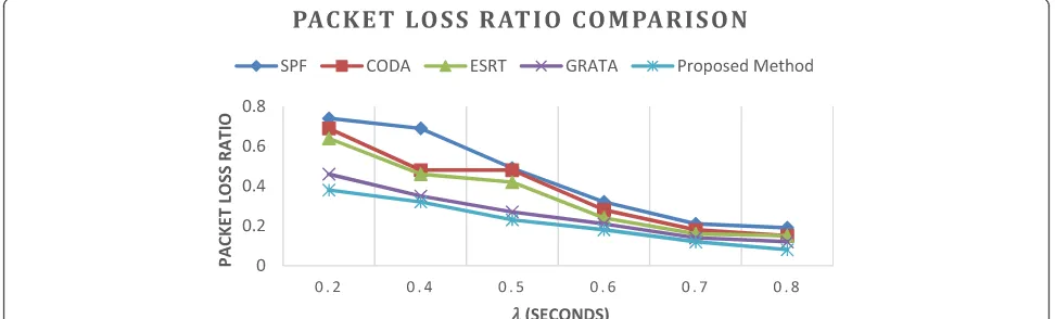
To assess the performance of the proposed algorithm, we simulate four congestion control schemes, including the shortest path first (SPF) method (a standard protocol for shortest path routing) and more sophisticated algorithms designed for large scale sensor network such as CODA [10], ESRT [11], and GRATA [16] in terms of packet loss Table 1 Packet loss ratio comparison
Algorithm λ(s)
0.2 0.4 0.5 0.6 0.7 0.8
SPF 0.74 0.69 0.49 0.32 0.21 0.19
CODA 0.69 0.48 0.48 0.28 0.18 0.15
ESRT 0.64 0.46 0.42 0.24 0.16 0.15
GRATA 0.46 0.35 0.27 0.21 0.14 0.12
Proposed 0.38 0.32 0.23 0.18 0.12 0.08
ratio, energy consumption, and end-to-end packet delay using the NS2 simulator. In addition, the influence of vari-ous values of traffic factors and data transmission rate are also considered.
The simulation parameters are set as follows: 100 homogeneous sensor nodes (including source nodes and sink nodes) are randomly distributed in a square region of 100 × 100 m with three sinks inside the coverage area. The nodes’communication radius is 20 m, which is con-sidered an effective coverage area for sensor nodes. The transmission rate is 250 kbps in scenarios of constant bit rate traffic and burst traffic. The range of channel con-tention window size is [1, 63]. The total buffer size is 20 data packets. The size of every packet is 50 Bytes. The IEEE 802.15.4 standard is used at the MAC and physical layers. Each node maintains traffic information of its neighbors by APs periodically and uses proposed algo-rithm to forward packets over optimal paths toward one of the sinks. Through several simulation rounds under high traffic condition, the weighted factors are α1= 0.7,
α2= 0.2,α3= 0.1, andφ= 0.7.
We setβ=1.5. With the choice ofVd(n) =ni, one finds
the upper and lower bounds of β are 2 and 1, respect-ively. A systematic analysis of the effects ofβon the sys-tem behavior is not trivial. However, we could use simulation to see the effect of β. It is seen that when β varies between 1.3 and 1.7, the system results are better.
This is because the proposed algorithm with sufficient weighting factor value could change the routing to dis-tribute traffic load.
The simulation results are compared with the SPF routing algorithm, CODA, ESRT, and GRATA to show the improvement in network performance with varied traffic rates.
5.1 Packet loss ratio
Figure 1 depicts packet loss ratios (with respect to time) associated with the five congestion control schemes. The x-axis denotes the various values of packet inter arrival times, while the y-axis denotes the packet loss ratio of the algorithms. The graph indicates that the proposed scheme outperforms the others due to its ability to pre-dict network conditions at the next hops in order to preempt potential congestions. In other words, the pro-posed algorithm has the capability to route packets around the congested area. In this scenario, traffic is generated following the exponential distribution with mean outcome set from = 0.2 to 0.8 s to show the vari-ous packet inter arrival times for packets based on the Poisson distribution. Table 1 denotes that our scheme significantly achieves the lower packet loss ratio com-pared to SPF, CODA, ESRT, and GRATA. This is be-cause the hops’information utilization scheme attempts to prevent forwarding packets to the next neighbors with high number of packets in the buffer and balanced network traffic as much as possible.
As shown in Table 1 for all methods, when the inter arrival time of packets is high, then the packet loss ratio will be low. This is because all algorithms are using the shortest path method to route packets, therefore, there is not a remarkable difference between various methods. However, when the inter arrival time of packets reduces, or in other words when the number of interval packets increases, the proposed method outperforms the other methods. The reason for our algorithm superiority is its ability to better predict network congestion landscape Table 2 Average energy consumption per bit
Algorithm λ(s)
0.2 0.4 0.5 0.6 0.7 0.8
SPF 0.74 0.69 0.49 0.32 0.21 0.19
CODA 0.69 0.48 0.48 0.28 0.18 0.15
ESRT 0.64 0.46 0.42 0.24 0.16 0.15
GRATA 0.51 0.39 0.33 0.21 0.14 0.1
Proposed 0.40 0.32 0.23 0.18 0.12 0.08
and adjust the data transmission rate in high traffic situations.
5.2 Energy consumption
In this subsection, we evaluate the medium energy con-sumption per bit, which is required to transmit a packet to the sink successfully, i.e., the proportion between the total taken energy at all nodes to send or transmit all packets and total bits in data packets which are received at the sink. The energy use is involved in communicat-ing and receivcommunicat-ing all packet types includcommunicat-ing data, ACK, and AP.
To judge the energy use of goods and services, we apply the same energy model as in [31], in which the packet transmission energy consumption is set to 50 NJ/bit*k+ 100 PJ/bit/m2*k*d2 and the packet reception energy is 50 NJ/bit*k, wherekis packet length anddis transmitted distance with respect to each packet. The initial energy for each node is set to 1 J. Figure 2 con-siders the average energy consumption per bit over five routing schemes with various values of packet inter ar-rival times.
As shown in Table 2, the proposed method consumes less energy than other methods. This difference is sig-nificant, because our method can reroute the paths and pass them from non-congested area. Furthermore, our scheme can adjust the packet transmission rate.
Figure 3 compares the average end-to-end packet delay through three sinks between the proposed algorithm with SPF, CODA, ESRT, and GRATA, respectively. For read-ability, the results are represented as the average
end-to-end delay of all nodes with six cases of packet inter arrival times in the range of 0.2 to 08 s.
From the graphs, we can conclude that the proposed routing scheme makes a smaller packet delay in com-parison with other schemes, especially when data trans-mission rate is high. This is because the proposed gradient-based scheme attempts to prevent forwarding packets to next neighbors with high number of packets in the buffer and balance network traffic as much as possible and adjust data transmission rate between two nodes. In particular, SPF has the highest end-to-end delay compared to other schemes. This causes a large amount of delay and energy consumption due to a lot of packets which are forwarded by the same nodes on the shortest paths. On the other hand, GRATA tries to re-duce the packet delay by utilizing the number of hops and the expected packet delay at one-hop neighbor. However, the routing scheme based on only one-hop in-formation can suffer from a lack of inin-formation about the possible congested areas. As it could be seen in the graphs, the end-to-end delay achieved by GRATA be-comes worse than the proposed scheme considerably when the network traffic increases. This is because the new method uses the traffic information to scatter the packets and adjust the data transmission rate (Table 3).
5.3 Efficient of weighted factors on network performance
The buffer thresholds decide the weighted factorsα1,α2, andα3for limiting the number of candidates participating the contest. The technique thus reduces the computation resource at sensor nodes. Nevertheless, this parameter is influenced by experimental trials; it is difficult to guar-antee an optimal effect on network operation. In this subdivision, we look at the impact of weighted factors on the packet delivery ratio under several traffic condi-tions. It should be noted that in our scheme, one-hop queue length is considered to be a more important factor than congestion degree and cumulative queue length. Thus,α1is always greater than or equal to the total of α2 andα3in simulation settings.
At first, the influence of α1(queue length field) is illus-trated in Figure 4 under traffic sending rate = 0.5 s through Table 3 Average end-to-end packet delay
Algorithm λ(s)
0.2 0.4 0.5 0.6 0.7 0.8
SPF 2.6 2.3 2 1.9 1.8 1.71
CODA 2.5 2.1 1.9 1.82 1.72 1.6
ESRT 2.18 2.02 1.8 1.75 1.65 1.55
GRATA 2.1 1.9 1.7 1.65 1.5 1.39
Proposed 1.8 1.6 1.53 1.5 1.4 1.2
a range of α1, whereas other traffic measurement factors are 0 (α2=α3= 0). We also show the SPF methods’packet delivery ratio in this figure. With a smallα1, it is difficult to obtain a high buffer threshold at parent nodes and our method will perform similar to SPF method. On the other hand, a very large α1indicates that the incoming packet is prevented from using the shortest path even though the current buffer at parent node is still small. This increases the packet end-to-end delay without improving the packet delivery ratio. Figure 4 shows that the high performance of our proposed system is ap-proximately obtained atα1= 0.7 (Table 4).
We infer that the influence of choosing factors de-pends on the current traffic condition in the network and forecasts the forwarding traffic with the congestion degree and the cumulative queue length. Now, we evalu-ate the influence ofα2,α3on the network performance, as illustrated in Figure 5. The traffic rate at each source is = 0.5 s. We consider α2= 0.2 andα4= 0.1 and com-pare these new values with the previous experiment re-sults. In instances of high traffic load, a remarkably higher value of all traffic information factors gets in-volved in routing decisions. The trade-off between one-hop and other traffic information (congestion degree and cumulative queue length) needs to be considered. Nevertheless, it is hard to see an optimalαratio because it depends strictly on current traffic status. Thus, a strat-egy founded on network traffic experience that dynamic-ally estimates this ratio after each point of time could be
a base of comparative study in future works. It can be seen that on average, when α1= 0.7, α2= 0.2, and α3= 0.1, the packet delivery ratio will be over 0.82. Neverthe-less, in general, in low traffic networks, small traffic factors reduce the issue of traffic information along the utilization field, as shown by Equation 7. Routing oper-ation then works in the same way as the shortest path routing. On the other hand, in congested networks, lar-ger values of traffic factors enhance the dynamic traffic property in choosing the next forwarder (Table 5).
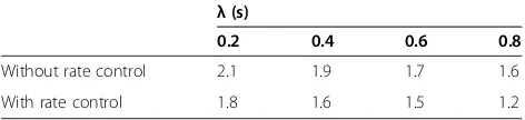
5.4 Effects of data transmission rate
Figure 6 shows the influence of rate adjusting strategy to average end-to-end delay with different packet enter ar-rival time. α, β variables in all experiments are similar. The graph indicates that congestion control with data transmission rate outperforms the others due to its ability to decrease or increase data transmission rate in con-gested or non concon-gested places. Clearly, with considering the data transmission rate factor in all experiments, energy consumption, and average end-to-end delay will also im-prove (Table 6).
6 Conclusions
In this paper, we proposed a hop-by-hop gradient-based routing scheme to evenly distribute traffic in WSNs with non-equivalent sink. The key concept herein is to utilize the number of hops and the current traffic loading of neighbors to make routing decisions. The proposed scheme Table 4 Packet delivery ratio with = 0.5 and different
amount ofα1 Algorithm α1
0 0.2 0.4 0.5 0.6 0.7 0.8 0.9 1
SPF 0.51 0.51 0.51 0.51 0.51 0.51 0.51 0.51 0.51
Proposed 0.51 0.59 0.61 0.63 0.70 0.77 0.70 0.60 0.52 ƛis value of packet inter arrival time.
Figure 5Compare packet delivery ratio with various values ofα2and with effect ofα2,α3.
Table 5 Compare packet delivery ratio with various value ofα1and with effect ofα2,α3
α1
0 0.2 0.4 0.5 0.6 0.7 0.8 0.9 1
α2=α3= 0 0.51 0.59 0.61 0.63 0.70 0.75 0.70 0.60 0.52
-reduces the number of packet retransmissions and packets dropped by preventing nodes with overloaded buffers from joining in routing calculation. Simulation results indicate that our proposed scheme improves network performance such as end-to-end packet delay, packet delivery ratio, and average energy consumption in comparison to other rout-ing schemes includrout-ing SPF, CODA, ESRT, and GRATA. To address practical concerns, the proposed routing algorithm can be easily implemented on existing devices without major changes.
The limitation of the new method is that the values of traffic factors (α,β, andφ) are chosen based on simulation experiments. Moreover, overhead is a common drawback of proposed algorithms. The proposed scheme needs in-formation about the number of hops and queue informa-tion supported from AP. Therefore, a part of network resource is used for sending/receiving this kind of broad-cast information. In future work, therefore, we plan to build an analytical model to find the optimal value for these weighted factors.
Moreover, some WSNs are application oriented, and different applications have different requirements. To conform to this diversity, an open framework is needed to consider other factors as well. We suggest that a gen-eral framework could be extended to optimize various other metrics through constructing other utilization fields and introducing additional mechanisms for per-formance enhancement. For example, we can extend our method to support priority-based applications
simultaneously through introducing an enhanced mech-anism. The packets from different applications can be assigned to different weights carried in the packet header and in the queue. The packet with light weight is well cached with the idle nodes, and higher priority packet with heavy weight travels along shorter paths to approach the sink as soon as possible. These may be possible subjects of future work in this direction.
Competing interests
The authors declare that they have no competing interests.
Author details
1
Department of Computer engineering, Science and Research Branch, Islamic Azad University, Tehran 46789-4113, Iran.2Computer engineering and information technology Department, Qazvin Branch, Islamic Azad University, Nokhbegan Blvd, Qazvin, Iran.3Computer engineering and information technology Department, Amirkabir University of Technology, Hafez Street, No. 424, Tehran, Iran.
Received: 6 September 2014 Accepted: 3 January 2015
References
1. P Rawat, KD Singh, H Chaouchi, JM Bonnin, Wireless sensor networks: a survey on recent developments and potential synergies. J. Supercomput. 68(1), 1–48 (2014)
2. M Gholipour, MR Meybodi, LA-mobicast: a learning automata based mobicast routing protocol for wireless sensor networks. Sens. Lett. 6(2), 305–311 (2008)
3. K Akkaya, M Younis, A survey on routing protocols for wireless sensor networks. Ad Hoc Netw.3(3), 325–349 (2005)
4. JN Al-Karaki, AE Kamal, Routing techniques in wireless sensor networks: a survey. Wireless communications, IEEE11(6), 6–28 (2004)
5. L Mottola, GP Picco, MUSTER: adaptive energy-aware multisink routing in wireless sensor networks. Mobile Computing, IEEE Transactions on 1012, 1694–1709 (2011)
6. V Shah-Mansouri, A-H Mohsenian-Rad, VWS Wong, Lexicographically optimal routing for wireless sensor networks with multiple sinks. Vehicular Technology, IEEE Transactions on 583, 1490–1500 (2009)
7. I Slama, J Badii, Djamal, in Wireless Communications and Networking Conference, Los Vegas, USA, 31March-3April, 2008. WCNC 2008, Energy efficient scheme for large scale wireless sensor networks with multiple sinks, (IEEE, 2008), p.2367–72
8. H Yoo, S Moonjoo, K Dongkyun, KH Kim. in Computers and
Communications (ISCC), 2010 IEEE Symposium on, Riccione, Italy, 22-25 June 2010. GLOBAL: A gradient-based routing protocol for load-balancing in
Figure 6Shows the influence of transmission rate adjustment in the average end-to-end delay.
Table 6 The influence of transmission rate adjustment in the average end-to-end delay
λ(s)
0.2 0.4 0.6 0.8
Without rate control 2.1 1.9 1.7 1.6
large-scale wireless sensor networks with multiple sinks, (IEEE, 2010), p. 556–562
9. C Sergiou, V Vassiliou, A Paphitis, Hierarchical tree alternative path (HTAP) algorithm for congestion control in wireless sensor networks. Ad Hoc Netw. 11(1), 257–272 (2013)
10. C-Y Wan, SB Eisenman, AT Campbell. in Proceedings of the 1st international conference on Embedded networked sensor systems, Los Angeles, CA, USA, 5-7 November 2003.CODA: congestion detection and avoidance in sensor networks, (ACM, 2003), p. 266–279
11. Y Sankarasubramaniam, ÖB Akan, IF Akyildiz. in Proceedings of the 4th ACM International Symposium on Mobile ad hoc Networking & Computing, Annapolis, MD, USA, 1-3 June 2003. ESRT: event-to-sink reliable transport in wireless sensor networks, (ACM, 2003), p. 177–188
12. S Rangwala, R Gummadi, R Govindan, K Psounis. in ACM SIGCOMM Computer Communication Review, Interference-aware fair rate control in wireless sensor networks, vol. 36, no. 4, (ACM, 2006), p. 63–74 13. T He, JA Stankovic, C Lu, and T Abdelzaher, In Distributed Computing
Systems, 2003. Proceedings. 23rd International Conference on, Providence, RI, USA, 19-23 May 2003. SPEED: a stateless protocol for real-time communication in sensor networks, (IEEE, 2003) p. 46–55
14. R Kumar, R Crepaldi, H Rowaihy, AF Harris, G Cao, M Zorzi, TF La Porta, Mitigating performance degradation in congested sensor networks. Mobile Computing, IEEE Transactions on 76, 682–697 (2008)
15. PP Pham, S Perreau, in INFOCOM 2003. Twenty-Second Annual Joint Conference of the IEEE Computer and Communications. IEEE Societies, Sunfrancisco, USA, 30 March- 3 April 2003. Performance analysis of reactive shortest path and multipath routing mechanism with load balance, vol. 1 (IEEE, 2003), p. 251–259
16. L Popa, C Raiciu, I Stoica, DS Rosenblum, in Network Protocols,2006. ICNP ’06. Proceedings of the 2006 14th IEEE International Conference on, Santa Barbara, California, USA, 12-15 November 2006. Reducing congestion effects in wireless networks by multipath routing, (IEEE, 2006), p. 96–105 17. C Intanagonwiwat, R Govindan, D Estrin, J Heidemann, F Silva, Directed
diffusion for wireless sensor networking. Networking, IEEE/ACM Transactions on 111, 2–16 (2003)
18. RM Pussente, VC Barbosa, An algorithm for clock synchronization with the gradient property in sensor networks. Journal of Parallel and Distributed Computing69(3), 261–265 (2009)
19. F Ren, T He, S Das, C Lin, Traffic-aware dynamic routing to alleviate congestion in wireless sensor networks. Parallel and Distributed Systems, IEEE Transactions on 229, 1585–1599 (2011)
20. DD Tan, D-S Kim, Kim, Dynamic traffic-aware routing algorithm for multi-sink wireless sensor networks. Wirel. Netw20, 1–12 (2013). doi:10.1007/s11276-013-0672-z
21. A Basu, A Lin, S Ramanathan, in Proceedings of the 2003 conference on Applications, technologies, architectures, and protocols for computer communications, Karlsruhe, Germany, 25-29 Aguest 2003. Routing using potentials: a dynamic traffic-aware routing algorithm, (ACM, 2003), p. 37–48 22. H Yoo, M Shim, D Kim, K H Kim, in Computers and Communications (ISCC),
2010 IEEE Symposium on, Riccione, Italy, 22-25 June 2010. GLOBAL: a gradient-based routing protocol for load-balancing in large-scale wireless sensor networks with multiple sinks, (IEEE, 2010), p. 556–562
23. P Huang, H Chen, G Xing, Y Tan, SGF: a state-free gradient-based forwarding protocol for wireless sensor networks. ACM Transactions on Sensor Networks (TOSN) 52, 14 (2009)
24. J Suhonen, M Kuorilehto, M Hannikainen, T D Hamalainen, in Personal, Indoor and Mobile Radio Communications, 2006 IEEE 17th International Symposium on, Helsinki, Finland, 11-14 September 2006. Cost-aware dynamic routing protocol for wireless sensor networks-design and prototype experiments, (IEEE, 2006), p. 1–5
25. PTA Quang, D-S Kim, Enhancing real-time delivery of gradient routing for industrial wireless sensor networks. Industrial Informatics, IEEE Transactions on 81, 61–68 (2012)
26. D Gao, T Zheng, S Zhang, OWW Yang, in Vehicular Technology Conference Fall (VTC 2010-Fall), 2010 IEEE 72nd, Ottawa, Canada, 6-9 September 2010. Improved gradient-based micro sensor routing protocol with node sleep scheduling in wireless sensor networks, (IEEE, 2010), p. 1–5
27. C Park, I Jung, in Information Science and Applications (ICISA), 2010 International Conference on, Seoul, Korea, 21-23 April 2010. Traffic-aware routing protocol for wireless sensor networks, (IEEE, 2010), p. 1–8
28. DD Tan, NQ Dinh, DS Kim, GRATA: gradient-based traffic-aware routing for wireless sensor networks. Wireless Sensor Systems IET 32, 104–111 (2013). doi:10.1049/iet-wss.2012.0083
29. EW Dijkstra, A note on two problems in connexion with graphs. Numer. Math.1(1), 269–271 (1959)
30. C Schurgers, MB Srivastava, in Military Communications Conference, 2001. MILCOM 2001. Communications for Network-Centric Operations: Creating the Information Force. IEEE, McLean, VA, USA, 28-31 October 2001. vol. 1, Energy efficient routing in wireless sensor networks, (IEEE, 2001), p. 357–361 31. WR Heinzelman, A Chandrakasan, H Balakrishnan, in System Sciences, 2000.
Proceedings of the 33rd Annual Hawaii International Conference on, Maui, Hawaii, USA, 4-7 January 2000. Energy-efficient communication protocol for wireless microsensor networks, (IEEE, 2000), p. 10
Submit your manuscript to a
journal and benefi t from:
7Convenient online submission
7Rigorous peer review
7Immediate publication on acceptance
7Open access: articles freely available online
7High visibility within the fi eld
7Retaining the copyright to your article