Modeling of the Micro-indentation Process to Create Microlens Array Features on a Mold.

(1)

ABSTRACT

GUNDYAL, SUMIT ANAND. Modeling of the Micro-indentation Process to Create Microlens Array Features on a Mold. (Under the direction of Dr. Mark Pankow).

Microlens arrays have a series of miniature lenses that are arranged in a two-dimensional grid on a supporting substrate. There are two main fabrication methods: direct and indirect.

The direct method involves heating the material up to its thermoplastic state or photopolymerizing of curable polymers by UV radiation followed by the formation of spherical features due to surface tension. However, it is difficult to control the size and precision of these features using this method. The indirect method which involves fabricating a mold having concave features and then using replication technologies to get the final lens has better control over the form accuracy but it is a complex process.

One of the indirect methods involves fabricating a mold having concave microlens features on it followed by replicating these features on to the substrate using injection molding. These concave microlens array features can be formed on metal alloys by rapidly indenting with a die having convex lens features to make the mold.

(2)

(3)

(4)

Modeling of the Micro-indentation Process to Create Microlens Array Features on a Mold.

by

Sumit Anand Gundyal

A thesis submitted to the Graduate Faculty of North Carolina State University

in partial fulfillment of the requirements for the degree of

Master of Science

Mechanical Engineering

Raleigh, North Carolina 2019

APPROVED BY:

__________________________ __________________________ Dr. Mark Pankow Dr. Thomas Dow

Committee Chair

Dr. Gracious Ngaile

(5)

ii

DEDICATION

(6)

iii

ACKNOWLEDGEMENTS

Firstly, I would like to thank Dr. Mark Pankow for providing me this opportunity and for all the guidance and inputs for the research.

My sincere thanks to Dr. Thomas Dow for the research assistantship position during my third semester.

Thanks to Anthony Wong for the constant push throughout the project and the help with the experiments.

Thanks to Ken Gerrard for the help with the MATLAB scripts and important inputs. Thanks to Dr. Gracious Ngaile for serving on my advisory committee.

Thanks to Phillip Strader for the help with the nanoindentation experiments and Keyence microscope training.

I would like to thank Alexander Sohn from Facebook Reality Labs for the generous funding and support for this research.

I am also grateful for the time in my BLAST Lab and thanks to all the lab mates for the help and support.

Finally, I would like to thank my family and friends at NC State for making my time in this university memorable.

(7)

iv

BIOGRAPHY

(8)

v

LIST OF TABLES

Table 2.1. Constant values in the Johnson cook viscoelastic model for Al 1100 H14. ...27 Table 3.2. Young’s modulus values from the four indentation tests with mean and the

standard deviation calculated. ...37 Table 3.3. Material properties of Al 1100 used in the simulation. ...49 Table 3.4. Material properties of glassy carbon extracted from the nanoindentation

experiments. ...53 Table 8.1. Summary of the die designs and indentation strategies for a 4K resolution display.

(11)

viii

LIST OF FIGURES

Figure 1.1. FE-SEM images of (a) square packed microlens arrays and (b) hexagonally packed microlens array with overlap between each individual lens [1]. ... 1 Figure 1.2. Trace of light rays through microlens arrays. ... 2 Figure 1.3. A 6x6 concave spherical lens features on a mold. Diameter of each

feature = 15.84 μm, pitch = 25 μm, depth = 15.84 μm. ... 4 Figure 1.4 (a) Indent profile showing depth error (b) comparison of indent profile and best

fitted curve of the same radius [11]. ... 5 Figure 1.5. SEM micrographs of indents after diamond turning: (a) depth of cut = 2 μm and

(b) depth of cut = 1 μm [11]. ... 6 Figure 1.6. Contour plot of seven indents with different pitches in simulation.

Coefficient k is the ratio of pitch (t) and final indent diameter (d) (k = t/d) [12]. ... 7 Figure 1.7. Contour plot of indents made at different pitches in the experiment after the

pileups were removed using micro-grinding process. Coefficient k is the ratio of pitch (t) and final indent diameter (d) (k = t/d) [12]. ... 7 Figure 1.8. Diamond die having structured features nano features in an area of

20 μm x 20 μm with cone like features. The diamond die was used for

nanocoining [13]. ... 8 Figure 1.9. SEM images of the nanofeatures on the electroless nickel part. (a) 5000x

(b) 2500x [13]. ... 9

Figure 2.1. Stress-strain curve of a hypothetical bilinear elastic-plastic material. ...13 Figure 2.2. Schematic representation of the finite element model of the rigid spherical die

and mold specimen. ...14 Figure 2.3. Mesh pattern used for the finite element model of the rigid spherical die and

(12)

ix Figure 2.4. Stress-Strain curve of a hypothetical bilinear material. ...16 Figure 2.5. Effect of varying Young’s modulus on the spring back and indentation force

required. ...17 Figure 2.6. Plot of the springback amount across the right half cross-section of the indent.

Spring back amount reduces with increasing Young’s modulus. ...18 Figure 2.7. Force vs displacement curve comparison for varying Young’s modulus. ...18 Figure 2.8. Cross-sectional view of the indent profile showing the pile-up of the right half of

the indent for varying Young’s modulus. Pile-up height increases with increasing Young’s modulus. ...19 Figure 2.9. Effect of varying yield stress on the spring back and indentation force required. ...20 Figure 2.10. Plot of the springback amount across the right half cross-section of the indent.

Springback amount increases with increasing yield stress. ...20 Figure 2.11. Force vs displacement curve comparison for varying yield stress...21 Figure 2.12. Cross-sectional view of the indent profile showing the pile-up of the right half of

the indent for varying yield stress. Pile-up height decreases with increasing yield stress. ...21 Figure 2.13. Effect of varying tangent modulus on the spring back and indentation force

required. ...22 Figure 2.14. Plot of the springback amount across the right half cross-section of the indent.

Springback amount increases with increasing tangent modulus. ...23 Figure 2.15. Force vs displacement curve comparison for varying tangent modulus. ...23 Figure 2.16. Cross-sectional view of the indent profile showing the pile-up of the right half

(13)

x Figure 2.19. Indent profile comparison for quasi static and fast indentation. ...28 Figure 2.20. Comparison of the force vs displacement curves for quasi-static and fast

indentation. ...29

Figure 3.1.Schematic representation of a nanoindentation test consisting of the

nanoindenter tip and the sample [21]. ...31 Figure 3.2. (a) Typical loading history of a load controlled nanoindentation test. (b) Typical

force-displacement output data recorded during a test. ...31 Figure 3.3. Schematic showing explanation of Bruker’s three-plate capacitive transducer

operation for accurate force application [22]. ...32 Figure 3.4. Different types of depths in a nano indent. he = surface displacement at the

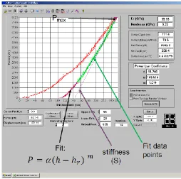
perimeter of contact (sink in), hr = final depth after load removal. ...33 Figure 3.5. Force-displacement curve of a nanoindentation test. P = α(h - hr)m is the curve

fit to the unloading curve. S is the slope of the unloading curve at Pmax (maximum force). ...33 Figure 3.6. Unloading curves at maximum load with the broken lines showing the

bowing of the unloading curves within the first few seconds of unloading [24]. ...35 Figure 3.7. Schematic representation of Berkovich indenter. ...36 Figure 3.8. Loading, unloading and hold regime of the nanoindentation experiment on

Al 1100 H14. ...37 Figure 3.9. Scanning probe microscopy (SPM) images of nano indents. ...38 Figure 3.10. Set 1 indents-force vs displacement curves with measured reduced modulus

values of Al 1100. ...38 Figure 3.11. Set 2 indents-force vs displacement curve with measured reduced modulus

(14)

xi Figure 3.12. Schematic diagram of the general operation of the nano-scratch tester when

taking a scratch measurement. ...40 Figure 3.13. Normal force vs lateral displacement plot of the nano scratch procedure. ...40 Figure 3.14. Time history plot of the ratio of lateral force and normal force on the indenter tip

during the nano-scratch test. ...41 Figure 3.15. Loading, unloading and hold regime of the nanoindentation experiment on

glassy carbon. Max Load = 10 mN. Load time = 30 secs. Unload time = 30 secs. Hold period = 20 secs. ...42 Figure 3.16. Force vs displacement curve with measured reduced modulus values of glassy

carbon. ...43 Figure 3.17. SPM images of glassy carbon surface before and after indentation. (a) Green

dots represent the spots at which indents are made. ...43 Figure 3.18. Schematic representation of the finite element model of the rigid axisymmetric

indenter and mold specimen for nanoindentation using Berkovich indenter. ...45 Figure 3.19. True stress versus true strain curve obtained from the tensile test of Al 1100

H14...46 Figure 3.20. Mesh pattern used for the finite element model of the rigid spherical indenter

and mold specimen. ...46 Figure 3.21. Comparison of force vs displacement curves obtained from the experiments

and the simulation. ...47 Figure 3.22. Comparison of force vs displacement curves obtained from the experiments

and the simulations. ...48 Figure 3.23. Height contour image of the Berkovich Indenter scanned under the Keyence

confocal microscope. ...49 Figure 3.24. Mesh pattern of (a) Berkovich indenter (Meshed with) and (b) Mold specimen

(15)

xii Figure 3.25. Comparison of force vs displacement curves obtained from the experiments

and the simulation. ...50 Figure 3.26. Z contour plot of the experimental and simulation nano indents using the

Berkovich indenter. (a) Experimental contour plot (b) Simulation contour plot. ...51 Figure 3.27. Error plot of experiment and simulation indent profiles. ...51 Figure 3.28. Comparison of force vs displacement curves obtained from the experiments

and the simulation. ...52 Figure 3.29. Von Mises stress distribution of the glassy carbon mold specimen at the end

of the loading period of the simulation. ...53

Figure 4.1. Contour image of the 2x2 die scanned under the Keyence VKX1100 confocal microscope. Approximate radius of each feature ≈ 15.84 μm. Distance between the center of each feature = 25.0164 μm. ...56 Figure 4.2. Experimental setup for the indentation experiment using the 2x2 die. ...56 Figure 4.3. Force vs displacement curves measured by the optical probe for the 2x2 die

indentation. ...57 Figure 4.4. Confocal laser microscope images of the indents made from a 2x2 die

(a) Indent 1 (b) Indent 2 (c) Indent 3. ...57 Figure 4.5. Mesh pattern of the 2x2 die and the mold specimen: Die meshed with C3D10M

elements and mold specimen meshed with C3D8R elements. ...59 Figure 4.6. Comparison of the force vs displacement comparison obtained from the

experiment and the simulation. ...60 Figure 4.7. (a) Experimental Z contour plot of the 2x2 indent. (b) Simulation Z contour

(16)

xiii Figure 5.1. A 6x6 concave spherical lens features on a mold. Diameter of each

feature = 15.84 μm, pitch = 25 μm, depth = 15.84 μm. ...63 Figure 5.2. CAD model of the 3x3 die. Die referred as 3x3 die (U). ...64 Figure 5.3. Plan view explaining the terminologies of column and rows to refer to indent. ...65 Figure 5.4. Preliminary indentation strategies where each square represents one lens

feature. The number represents the indent order and the gray represents the current indent. 3x3 die (U) is used for the indentation. ...65 Figure 5.5. Mesh pattern of the 3x3 die and the mold specimen: Die meshed with C3D10M

elements and Mold specimen meshed with C3D8R elements. ...66 Figure 5.6. Three feature step over. (a) Desired contour plot. (b) Simulation contour plot. (c)

Error plot (actual profile – desired profile). (d) The cross-section view across A-A’ of desired plot shown in (a). (e) The cross-section view across A-A’ of

simulation plot shown in (b). (f) Comparison of the desired, simulation and error plot across cross-section across A-A’. ...69 Figure 5.7. Two feature step over. (a) Desired contour plot. (b) Simulation contour plot.

(c) Error plot (actual profile – desired profile). (d) The cross-section view across A-A’ of desired plot shown in (a). (e) The cross-section view across A-A’ of

simulation plot shown in (b). (f) Comparison of the desired, simulation and error plot across cross-section across A-A’. ...70 Figure 5.8. One feature step over. (a) Desired contour plot. (b) Simulation contour plot.

(c) Error plot (actual profile – desired profile). (d) The cross-section view across A-A’ of desired plot shown in (a). (e) The cross-section view across A-A’ of

(17)

xiv Figure 5.9. (a) 1x3 die with each feature of radius 15.84 μm and the center to center

distance between each feature 25 μm (b) one feature stepover indentation

strategy with the 1x3 die. ...72 Figure 5.10. (a) 4x4 die with each feature of radius 15.84 μm and the center to center

distance between each feature 25 μm (b) one feature stepover indentation

strategy with the 4x4 die. ...73 Figure 5.11. Simulation contour plot for a 1x3 die indentation using the indentation strategy

in Figure 5.9 (b). ...74 Figure 5.12. Error contour plot for a 1x3 die indentation using the indentation strategy in

Figure 5.9 (b). ...74 Figure 5.13. Simulation contour plot for a 4x4 die indentation using the indentation strategy

in Figure 5.10 (b). ...75 Figure 5.14. Error contour plot for a 1x3 die indentation using the indentation strategy in

Figure 5.10 (b). ...75 Figure 5.15. Indentation scheme A: Schematic of a one feature stepover indentation strategy

with a total of sixteen indentations steps to form a 6x6 arrays of indents. The grey shade represents the current position of the die and the number in the cells represents the order of the indentation step. 3x3 die (U) is used for the

indentation. ...77 Figure 5.16. 6x6 desired indent arrays plot for the indentation scheme A. ...79 Figure 5.17. Simulation contour plot of the indent arrays for indentation scheme A at the end

of the indentation step 4. ...80 Figure 5.18. Error contour plot and comparison of different cross section views parallel to the

X-axis using the indentation scheme A at the end of indentation step 4. ...81 Figure 5.19. Error contour plot and comparison of different cross section views parallel to the

(18)

xv Figure 5.20. Schematic of the indentation steps 1 to 4 of the indentation scheme A,

explaining the behavior of the material flow. Green dashed box indicates no indent cavity below it. Red dashed box indicates the compressional deformation in the indents formed due to that indentation step. Arrows indicate the direction of the material flow causing compressional deformation during indentation. ...83 Figure 5.21. Simulation contour plot for indentation scheme A at the end of the indentation

step 8. ...84 Figure 5.22. Error contour plot and comparison of different cross section views parallel to

the X-axis using the indentation scheme A at the end of indentation step 8. ...85 Figure 5.23. Error contour plot and comparison of different cross section views parallel to

the Y-axis using the indentation scheme A at the end of indentation step 8. ...86 Figure 5.24. Schematic of the indentation steps 5 to 8 of the indentation scheme A,

explaining the behavior of the material flow. Green dashed box indicates no indent cavity below it. Blue dashed box indicated the presence of compressional deformation in the indent caused in the previous indentation step. Red dashed box indicates the compressional deformation in the indents formed due to that indentation step. Arrows indicate the direction of the material flow causing

compressional deformation during the indentation. ...87 Figure 5.25. Simulation contour plot for indentation scheme A at the end of the indentation

step 12. ...88 Figure 5.26. Error contour plot and comparison of different cross section views parallel to

the X-axis using indentation scheme A at the end of indentation step 12. ...89 Figure 5.27. Error contour plot and comparison of different cross section views parallel to

the Y-axis using indentation scheme A at the end of indentation step 12. ...90 Figure 5.28. Schematic of the indentation steps 8 to 12 of the indentation scheme A,

(19)

xvi below it. Blue dashed box indicates the presence of compressional deformation in the indent caused in the previous indentation step. Red dashed box indicates the compressional deformation in the indents formed due to that indentation step. Arrows indicate the direction of the material flow causing compressional deformation during indentation. ...91 Figure 5.29. Comparison of the form error of indents across cross sections parallel to the

X axis using the indentation scheme A. ...92 Figure 5.30. Comparison of the form error of indents across cross sections parallel to the

Y axis using the indentation scheme A. ...92

Figure 6.1. 3x3 die having features with equal radius and different depth. Die referred as

3x3 die (R).

Depth (A) < Depth (B) < Depth (C) < Depth (D) = 15.84 μm Depth (D) = 15.84 μm, Depth (C) = 15.84 μm – 2 μm = 13.84 μm, Depth (B) = 15.84 μm – 4 μm = 11.84 μm,

Depth (A) = 15.84 μm – 6 μm = 9.84 μm Radius (A) = Radius (B) = Radius (C) = Radius (D). ...95

Figure 6.2. 3x3 die having features with unequal radius. Die referred as 3x3 die (D). Radius (D) = 15.84 μm, Radius (C) = 15.84 μm – 2 μm = 13.84 μm,

Radius (B) = 15.84 μm – 4 μm = 11.84 μm, Radius (A) = 15.84 μm – 6 μm = 9.84 μm ...95 Figure 6.3. Indentation scheme B: Schematic of a one feature stepover indentation strategy

(20)

xvii Figure 6.2. The alphabet labels in each cell represents the last feature that

indented in that spot before the current indentation step. The die used in this

scheme is any one of 3x3 progressive dies. ...96 Figure 6.4. Mesh pattern of the 3x3 progressive die shown in Figure 6.1 meshed with

C3D10M elements. ...98 Figure 6.5. Mesh pattern of the 3x3 progressive die shown in Figure 6.2 meshed with

C3D10M elements. ...98 Figure 6.6. 6x6 desired indent plot for the indentation scheme B. ... 100 Figure 6.7. Simulation contour plot for the 3x3 die (R) at the end of indentation step 8

using the indentation scheme B. ... 102 Figure 6.8. Error contour plot of the indent arrays and comparison of different cross section

views parallel to the X-axis formed with the 3x3 die (R), using indentation

scheme B at the end of indentation step 8. ... 103 Figure 6.9. Error contour plot of the indent arrays and comparison of different cross section

views parallel to the Y-axis formed with the 3x3 die (R), using indentation

scheme B at the end of indentation step 8. ... 104 Figure 6.10. Schematic of the indentation steps 5 to 8 of the indentation scheme B,

explaining the behavior of material flow. Green dashed box indicates no indent cavity below it. Blue dashed box indicates the presence of indents with shallower depth. Red dashed box indicates the compressional deformation in the indents formed due to that indentation step. Arrows indicate the direction of the material flow causing compressional deformation during indentation. ... 105 Figure 6.11. Simulation contour plot for the 3x3 die (R) at the end of indentation step 16

(21)

xviii Figure 6.12. Error contour plot of the indent arrays and comparison of different cross

section views parallel to the X-axis formed with the 3x3 die (R), using

indentation scheme B at the end of indentation step 16. ... 107 Figure 6.13. Error contour plot of the indent arrays and comparison of different cross

section views parallel to the Y-axis formed with the 3x3 die (R), using

indentation scheme B at the end of indentation step 16. ... 108 Figure 6.14. Schematic of the indentation steps 13 to 16 of indentation scheme B,

explaining the behavior of the material flow and the cause of compressional deformation. Green dashed box indicates no indent cavity below it. Blue dashed box indicates the presence of indents with shallower depth. Red dashed box indicates the compressional deformation in the indents formed due to that indentation step. Arrows indicate the direction of the material flow

causing compressional deformation during indentation. ... 109 Figure 6.15. Simulation contour plot for the 3x3 die (D) at the end of indentation step 8

using the indentation scheme B. ... 110 Figure 6.16. Error contour plot of the indent arrays and comparison of different cross

section views parallel to the X-axis formed with the 3x3 die (D), at the end of

indentation step 8 using indentation scheme B. ... 111 Figure 6.17. Error contour plot of the indent arrays and comparison of different cross

section views parallel to the Y-axis formed with the 3x3 die (D), at the end of

indentation step 8 using indentation scheme B. ... 112 Figure 6.18. Simulation contour plot for the 3x3 die (D) at the end of indentation step 16

using the indentation scheme B. ... 113 Figure 6.19. Error contour plot of the indent arrays and comparison of different cross

section views parallel to the X-axis formed with the 3x3 die (D), at the end of

(22)

xix Figure 6.20. Error contour plot of the indent arrays and comparison of different cross

section views parallel to the Y-axis formed with the 3x3 die (D), at the end of

indentation step 16 using indentation scheme B. ... 115 Figure 6.21. Error plot comparison of indent arrays formed with 3x3 die (R) and with a

3x3 die (D). Cross sections parallel to the X axis compared at the end of

indentation step 16 of the indentation scheme B... 117 Figure 6.22. Error plot comparison of indent arrays formed with 3x3 die (R) and with a 3x3

die (D). Cross sections parallel to the Y axis compared at the end of indentation step 16 of the indentation scheme B. ... 118 Figure 6.23. Error plot comparison of indent arrays formed with a 3x3 die (U) and with a 3x3

(R). Cross sections parallel to the X axis compared at the end of indentation step 12 of the indentation scheme A and indentation scheme B respectively. ... 119 Figure 6.24. Error plot comparison of indent arrays formed with a 3x3 die (U) and with a

3x3 (R). Cross sections parallel to the Y axis compared at the end of indentation step 12 of the indentation scheme A and indentation scheme B respectively. ... 120

Figure 7.1. Indentation scheme C: Schematic of an indentation scheme with two feature stepover every successive indentation step. The grey shade represents the current position of the die and the number represents the order of the

indentation step. Letter ‘Y’ represents the presence of compressional deformation in the indents due to previous indentation steps and the letter ‘N’ represents

reduced compressional deformation in the indent. ... 122 Figure 7.2. Indentation scheme D: Schematic of an indentation scheme with two feature

(23)

xx of the die and the number represents the order of the indentation step. Letter ‘Y’ represents the presence of compressional deformation in the indent due to previous indentation steps and the letter ‘N’ represents reduced compressional deformation in the indent. ... 123 Figure 7.3. (a) Simulation plot at the end of the indentation step 6 of indentation scheme B.

(b) Error plot at the end of indentation step 6 of indentation scheme B. ... 124 Figure 7.4. (a) Simulation plot at the end of the indentation step 12 of indentation scheme B.

(b) Error plot at the end of indentation step 12 of indentation scheme B. ... 125 Figure 7.5. (a) Simulation plot at the end of the indentation step 9 of indentation scheme C.

(b) Error plot at the end of indentation step 9 of indentation scheme C. ... 126 Figure 7.6. (a) Simulation plot at the end of the indentation step 13 of indentation scheme C.

(b) Error plot at the end of indentation step 13 of indentation scheme C. ... 126 Figure 7.7. Design of new die with three features added to the 3x3 die (U). This modified die

(24)

1

1. INTRODUCTION

1.1. Motivation

Microlens arrays have a series of miniature lenses that are arranged in a two-dimensional grid on a supporting substrate. Individual lenses can have circular apertures with no overlap between each other and can be placed in a hexagonal or square packed arrangement. If an overlap is allowed between each of the individual lenses, square apertures and hexagonal apertures can be formed. Fill-factor (active refracting area) up to 100 % can be achieved by increasing the overlap between each individual lenses. Figure 1.1 (a) and Figure 1.1 (b) shows an example of a square packed lens arrays and hexagonally packed lens arrays [1].

Figure 1.1. FE-SEM images of (a) square packed microlens arrays and (b) hexagonally packed microlens array with overlap between each individual lens [1].

(25)

2 technologies. Microlens arrays are also used in light field technology which is used to create a virtual reality which a human eye cannot distinguish from the real world. The main motivation of this work is to devise a method to fabricate microlens arrays for the Virtual Reality (VR) headsets.

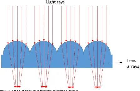
Figure 1.2. Trace of light rays through microlens arrays.

(26)

3 The indirect method of micro-lens fabrication requires the fabrication of the mold with concave features. This mold is then used to create the final lens array using techniques such as injection molding, hot embossing or UV molding. The form accuracy of the final micro-lens array is directly dependent on the precision of the geometry of these concave features. MEMs based technologies and ultraprecision machining are two categories in which these methods are classified. The standard MEMS methods utilize photolithography to generate patterns on the mask layer and chemical reactions to etching the curvature of microlens onto the substrate [5-7]. However, this approach requires expensive equipment and complicated procedures. Ultraprecision machining technologies utilize diamond micro-milling and single point diamond turning to fabricate microstructures and nanostructures with good uniformity in a large area [8-10]. Good surface roughness of Ra 5 nm is achieved. However, this method requires each micro-lens to be prepared one by one which increases the operation time and cost. An alternative of high-speed indentation using spherical convex dies is one of the methods to create concave spherical features on the mold.

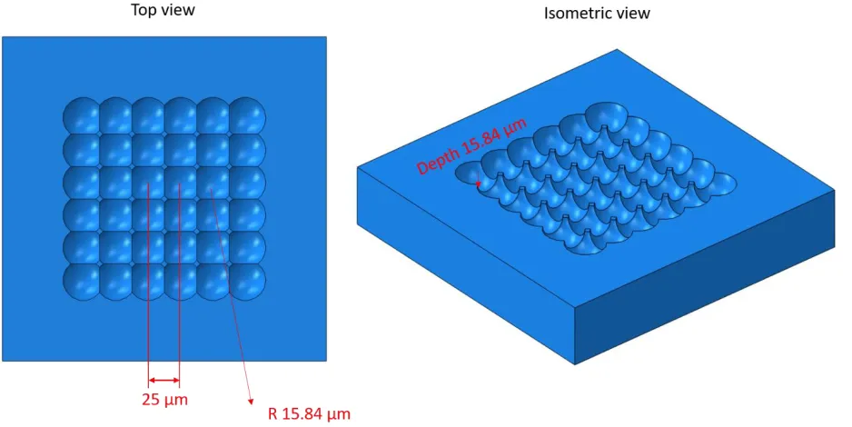
This work specifically focuses on investigating the process of fabricating a mold by indentation of convex spherical dies to create concave spherical features. Indentations at a frequency of 1 KHz are being aimed. This work, however, investigates indentations carried out quasi-statically. Figure 1.3 shows the required specifications of the microlens arrays. Finite element analysis is used to perform indentation simulations to understand the plastic flow of the

(27)

4 pile-up will build-up to the point where it could impede the movement of the impactor and change the final shape of the indent. Also, the pile-up from one indent will change the shape of previously made indents in that area. Some researchers have attempted to solve the form errors due to the elastic deformation of the die and the elastic springback of the mold. However, the issue of compressional deformation of the surrounding indents caused due to the close-packed arrangement of the lens features is not yet studied.

Figure 1.3. A 6x6 concave spherical lens features on a mold. Diameter of each feature = 15.84

μ

m, pitch = 25

μ

m, depth = 15.84

μ

m.

1.2. Research background

(28)

5 have shown clearly in Figure 1.4 (a) the depth error of the indent formed after 5 indentations in the same place due to the springback of the mold material and the elastic deformation of the machine elements including the die holder and the tool post. The nominal indentation depth is 20 μm, but the actual depth achieved is 11 μm. Figure 1.4 (b) also shows that a form error of approximately 0.65 μm is evident by fitting a curve of the same radius to the indent profile. The effect of diamond turning to remove the material pile-ups at different depth of cuts is also discussed. It is shown that diamond turning at higher depth of cut leads to the formation of exit burrs as showninFigure 1.5(a

)

and Figure 1.5(b). The pitch of the indents studied in this paper is high enough so that no interference is caused between adjacent indents. This ensures that the shape of the surrounding indents is not disturbed.

(a) (b)

(29)

6 (a) (b)

Figure 1.5. SEM micrographs of indents after diamond turning: (a) depth of cut = 2 μm and (b) depth of cut = 1 μm [11].

(30)

7 form error was calculated by subtracting the ideal indent profile from the actual indent profile. By compensating the form error to the die shape the maximum form error was reduced from 2.6% of the indent depth to 0.0075% of the indent depth.

Figure 1.6. Contour plot of seven indents with different pitches in simulation. Coefficient k is the ratio of pitch (t) and final indent diameter (d) (k = t/d) [12].

Figure 1.7. Contour plot of indents made at different pitches in the experiment after the pileups were removed using micro-grinding process. Coefficient k is the ratio of pitch (t) and final indent diameter (d) (k = t/d) [12].

(31)

8 create features which are tightly packed with a pitch less than the diameter of a single indent.To create arrays of closely packed indents, a die with a single feature will not help as it would not prevent the compressional deformation of adjacent indents. A die having multiple features which implements novel indentation strategies must be explored.

The Precision Engineering Consortium (PEC) at North Carolina State University had devised a new process called which involved fabricating high quality ordered nanofeatures. E Zdanowicz et al [13] used a diamond die having structured nanofeatures in an area of 20 μm x

20 μm to transfer features to a mold surface as shown in Figure 1.8. The nanocoining process was carried on a 6 mm wide ring on a 1.25” diameter stainless steel plated with a 380 μm thick

layer of electroless nickel sample at a rate of 1 kHz by using an actuating system developed by

the T.A Dow et al [14] at the PEC. Figure 1.9 shows the SEM image of the nanofeatures fabricated on the electroless nickel sample. The image shows mold material sticking out of the surface

around the hole. This phenomenon is different from pile-up that would be experienced in the case

of microindentation.

Figure 1.8. Diamond die having structured features nano features in an area of 20 μm x 20 μm

(32)

9 (a) (b)

Figure 1.9. SEM images of the nanofeatures on the electroless nickel part. (a) 5000x (b) 2500x [13].

The present work aims at features much larger than those attempted for the nanocoining process. The increased scale of the size of the features brings with it its own challenges, but the previous work at the PEC lays a general framework upon which the present work will be based.

(33)

10 the simulations had significantly lower loads than the experiments. Warren and Guo [17] attributes the lower loads to the machining-induced residual stresses that significantly affects the displacement curves. H. Lee et al [18] showed that friction coefficient does not affect the force-displacement curves.

1.3. Research objectives

The objective of this research is to investigate the above issues pertaining to the fabrication of closely packed concave spherical features on a mold which are much smaller than that considered by Jiwang Yan et al [11] and Yaqun Bai et al [12] but considerably larger than that fabricated by the PEC and devise new solutions to mitigate those issues.

Chapter 2 discusses the effect of tweaking different parameters like the material

properties of a hypothetical material, frictional contact between the die and the substrate, and the strain-rate dependent mold material on the indentation shape and the indentation forces required. This study could help in deciding an ideal mold material which causes lesser springback and pile-ups.

Chapter 3 discusses a detailed verification study of the FEA model of nanoindentation

and corresponding nanoindentation experiments. Two important response quantities were measured from the experiments to help in the correlation of the FEA models namely the force versus displacement curves and the indent profile. These verification studies helped in calibrating the material properties of the mold and the die for the microindentation procedure.

Chapter 4 discusses the validation step of the FEA model of indentation using a 2x2 die

modeled using the calibrated material properties of the mold and the die from Chapter 3. With this chapter the verification and validation of FEA models with the experimental data is accomplished and confidence is gained in the predictive capability of the computational model.

Chapter 5 deals with designing dies having multiple features of uniform size and

(34)

11 behavior of material flow during different indentation strategies is discussed and the factors affecting the form accuracy of the indents in the arrays is studied. The work in this chapter provides some important insights into the mechanism of indentation which sets up the framework for future studies to help in improving the form accuracy of the indents.

Chapter 6 investigates the indentation process for forming arrays of micro features on the

mold using a die having features with progressively increasing size. The form accuracy of the indents formed using these dies is compared to that from the dies used in chapter 5. The behavior of material flow and the mechanism causing the compressional deformation in the indents is studied. The advantages and of using the progressive multi-featured die is discussed.

Chapter 7 attempts at devising new indentation strategies with the aim to reduce the

compressional deformation in the indents which is a major cause for the deterioration of the form errors of the indents. The die shape compensation technique is briefly discussed which would help in mitigating the form errors due to springback of the indents and the elastic deformation of the die.

Chapter 8 provides a brief summary of the conclusion of the major findings in this thesis

(35)

12

2. MATERIAL PARAMETER STUDY

The microindentation process involves pressing a die (in this case with lens features) on a relatively softer mold material to cause permanent deformation. Materials with high compressive yield stress are ideal for a die which helps prevent it from deforming plastically during indentation. Glassy carbon is chosen as the die material as it has high compressive strength and high hardness which makes it suitable for a die. Also, as glassy carbon is amorphous, (Focussed Ion Beam) FIB milling process will be more uniform than a material with grainy structure. Finally, the rate of removing material is about 5 times that of the diamond. To understand the effect of mold material on the final indent shape and the indention force required it is necessary to do a material parameter study to understand the effect of different material parameters on the indentation shape and indentation loads. This would also aid in deciding a suitable mold material. Finally, the effect of friction and strain rate dependency of the mold material is also discussed.

This study is conducted by developing a computational model of a quasi-static microindentation process of a rigid spherical die of radius 20 μm indenting into a rectangular cuboid. The material properties that would be varied are given in Table 2.1.

Table 2.1 Material parameters to be studied for a quasi-static microindentation process.

Young’s modulus Yield stress Tangent modulus

E

σy

E

t

(36)

13 unloading. For softer mold materials, as the strain in the mold enters the plastic region the material is pushed out of the indent cavity which leads to pile-up around the periphery of the indent. Indentation force is the reaction force experienced by the die when the indentation is progressing. The role of friction on the indent shape and the indentation force required will be explored as well. Strain rate dependent behavior will also be addressed.

Figure 2.1. Stress-strain curve of a hypothetical bilinear elastic-plastic material.

2.1. Finite element modeling

(37)

14 A 2D axisymmetric model was employed for the finite element modeling of the indentation process of a rigid spherical die on a mold specimen. The schematic representation of the model is shown in Figure 2.2. The die was meshed with RAX2 elements: 2 node linear axisymmetric rigid link elements and the mold specimen was meshed with CAX4R elements: 4 node bilinear axisymmetric quadrilateral, reduced integration, hourglass control elements as shown in Figure 2.3. The mold specimen was meshed with uniform density. Non-linear geometry option was used in the finite element simulation. Arbitrary Lagrangian Eulerian (ALE) adaptive mesh domains was defined for the mold specimen as it involved large deformations. Surface-to-surface contact condition was used with the die as the master surface and the mold surface as the slave surface since a master surface can penetrate the slave surface. Frictionless contact was considered. Isotropic hardening material behavior was used to model the plasticity region of the material. The bottom surface of the mold was fixed by constraining all the degrees of freedom. The nodes on the axis of symmetry were applied with the X symmetry boundary condition by restraining the degrees of freedom: U1, UR2, and UR3.

Figure 2.2. Schematic representation of the finite element model of the rigid spherical die and mold specimen.

The simulations were performed by indenting a rigid die of radius 20 μm to a depth of 10

(38)

15 is displaced at a constant velocity. Comparison of the kinetic energy and internal energy of the system obtained from the output results shows that the kinetic energy is less than 5% of the internal energy. This ensures the inertial effects are kept to the minimum.

Figure 2.3. Mesh pattern used for the finite element model of the rigid spherical die and mold specimen.

(39)

16

Figure 2.4. Stress-Strain curve of a hypothetical bilinear material. 2.1.1. Young’s modulus as the input parameter

(40)

17 Figure 2.5. Effect of varying Young’s modulus on the spring back and indentation force required.

As Young’s modulus is increased the spring back amount is expected to reduce considerably while the indentation force required is expected to increase by a negligible amount. Young’s modulus of 75 GPa, 60 GPa, and 45 GPa are used for the first study. As can be seen in

(41)

18 Figure 2.6. Plot of the springback amount across the right half cross-section of the indent. Spring back amount reduces with increasing Young’s modulus.

(42)

19 Figure 2.8. Cross-sectional view of the indent profile showing the pile-up of the right half of the indent for varying Young’s modulus. Pile-up height increases with increasing Young’s modulus.

2.1.2. Yield stress as the input parameter

In the second study, Young’s modulus and the tangent modulus is kept constant at 75 GPa and 0.1 GPa respectively. The effect of varying yield stress on the indent shape and the indentation force required is observed. The results can be anticipated in a bilinear stress-strain curve of a hypothetical material as shown in Figure 2.9.

(43)

20

Figure 2.9. Effect of varying yield stress on the spring back and indentation force required.

(44)

21 Figure 2.11. Force vs displacement curve comparison for varying yield stress.

(45)

22 2.1.2. Tangent modulus as the input parameter

In the third study, Young’s modulus and the yield stress is kept constant at 75 GPa and 120 MPa respectively. The effect of varying the tangent modulus on the indent shape and the indentation force required is observed. The results can be anticipated in a bilinear stress-strain curve of a hypothetical material as shown in Figure 2.13.

(46)

23 Figure 2.14. Plot of the springback amount across the right half cross-section of the indent. Springback amount increases with increasing tangent modulus.

(47)

24 Figure 2.16. Cross-sectional view of the indent profile showing the pile-up of the right half of the indent for varying tangent modulus. No direct correlation for the pile-up and the tangent modulus exists.

(48)

25 Table 2.2. Summary of the material parameter study. ↑ denotes an increasing value. ↓ denotes a decreasing value. ≈ denotes approximately equal values.

Indentation Outputs

Material parameters Pile-up height Spring back Indentation force

Elastic modulus ↑ ↑ ↓ ≈

Tangent modulus ↑ ↓ ↑ ↑

Yield stress ↑ ↓ ↑ ↑

2.1.3. Effect of friction

Friction between the die and the mold specimen plays a major role in affecting the pile-up height and spread around the die whereas it has no significant effect on the indentation force required. Material properties obtained from the tensile test of Al 1100 were used for the material definition of Al 1100 in Abaqus. Isotropic hardening rule is employed to model the plasticity region of Al 1100. The same setup as shown in Figure 2.2 and Figure 2.3 is used for this study.

(49)

26 Figure 2.17. Pile-up height and spread comparison for varying friction coefficient.

(50)

27 2.1.4. Effect of strain rate dependent behavior of Al 1100 H14 on micro-indentation

Al 1100 H14 is a positive strain rate sensitive material. A positive strain rate sensitive material experiences an increase in the yield stress as the strain rate increases. Johnson-Cook material model is generally used for computational analysis of the impact and the penetration related problems involving ductile materials. For high-speed indentation process, this would be an ideal model. The Johnson-Cook elastoviscoplastic model is given by Equation 2.1 which involves an independent factor of strain hardening, strain rate hardening and thermal softening. A, B and C are material constants whereas n is a hardening exponent and m is a softening exponent. σ is equivalent Von Mises stress.

𝜀

pl is the equivalent plastic strain. ε̇is the equivalent plastic strain rate. 𝜀̇0is reference strain rate which is equal to 1 s-1. T is a non-dimensional

temperature which is a function of room temperature.

Equation 2.1 The values of these constants are obtained by a series of tensile test experiments conducted at various strain rates by Sonika Sahu et al [20]. These constants are presented in Table 2.1.

Table 2.1. Constant values in the Johnson cook viscoelastic model for Al 1100 H14.

A B C n m Ɛ̇0

114 49.79 0.001 0.197 0.859 1

(51)

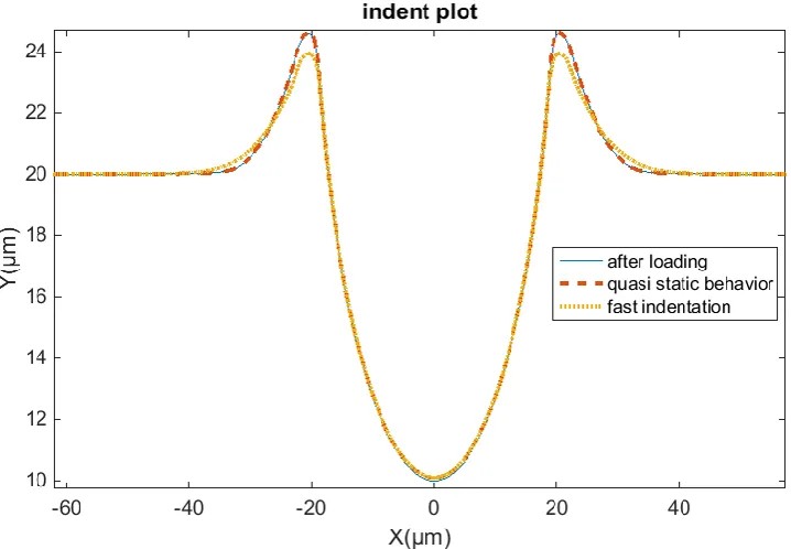
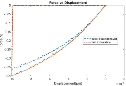
28 with a rate-dependent material model is used to model the plasticity of the Al 1100 mold. Figure 2.19 shows that there is no significant difference in the amount of spring back for quasi-static indentation and fast indentation. However, as the material is positive strain sensitive, the yield stress during high strain rate indentation is larger than that during quasi-static indentation and hence the pile-up experienced will be lesser. This phenomenon can be observed in Figure 2.20. Similarly, the force vs displacement plot in Figure 2.20 shows that faster indentation

experiences higher indentation force.

(52)

29 Figure 2.20. Comparison of the force vs displacement curves for quasi-static and fast indentation. 2.2. Conclusion

(53)

30

3. CORRELATION OF NANOINDENTATION EXPERIMENTS AND FINITE ELEMENT

SIMULATIONS

Verification and validation of microindentation experiment and finite element simulation is important to gain confidence in the predictive capabilities of the FEA models. Accurate prediction of the final indent shape and the force vs displacement curves will aid in designing the final die and developing indentation strategies. For this purpose, initially, nanoindentation experiments were conducted on Al-1100- H14 sample and glassy carbon sample using Hysitron TI-980

Triboindenter provided by the Analytical Instrumentation Facility (AIF) at North Carolina State University and finite element models were developed to validate these experiments. This potentially helped in calibrating the material properties of Al 1100 and glassy carbon.

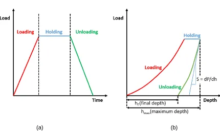
3.1. Nanoindentation

(54)

31 Figure 3.1.Schematic representation of a nanoindentation test consisting of the nanoindenter tip and the sample [21].

(a) (b)

(55)

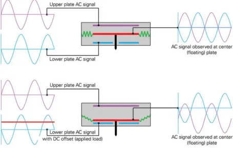
32 Figure 3.3. Schematic showing explanation of Bruker’s three-plate capacitive transducer operation for accurate force application [22].

(56)

33 Figure 3.4. Different types of depths in a nano indent. he = surface displacement at the perimeter of contact (sink in), hr = final depth after load removal.

Figure 3.5. Force-displacement curve of a nanoindentation test. P = α(h - hr)m is the curve fit to

the unloading curve. S is the slope of the unloading curve at Pmax (maximum force).

(57)

34 function A(hc) at hmax reduced elastic modulus (Er) and hardness (H) can be calculated from Equation 3.2 [23] and Equation 3.3 [23]. The relationship between the reduced modulus and the elastic modulus is given by Equation 3.4 [23].

A(hc) = Co(hc)2 + C1(hc) + C2(hc)1/2 + C3(hc)1/4 + C4(hc)1/8 + C5(hc)1/6 Equation 3.1

E

r

=

√π

2 S

√A(hc)

Equation 3.2

H

=

Pmax

A(hc)

Equation 3. 3

Equation 3.4

(58)

35 Figure 3.6. Unloading curves at maximum load with the broken lines showing the bowing of the unloading curves within the first few seconds of unloading [24].

3.2. Nanoindentation experiments

Nanoindentation tests use a standard diamond indenter tip which is driven into the different regions of the sample surface by increasing the normal load. Force-displacement data recorded during the test using high-resolution instruments are used to determine Young’s modulus, hardness, and the elastic-plastic deformation. For this study, a Berkovich diamond indenter tip is used. As glassy carbon is a hard material (340 HV) a Berkovich tip is a suitable geometry for an indenter to make an indentation deep enough to extract force-displacement data. The geometry of the Berkovich indenter is shown in Figure 3.7. Scratch tests were also performed to find the friction coefficient between diamond and Al 1100 sample which would later be used in the finite element simulations.

(59)

36 The relationship between reduced elastic modulus and Young’s modulus is given by the Sneddon relationship Equation 3.4 where E and

ν

are the elastic modulus and Poisson's ratio of the test

material, Ei and

ν

i are the elastic modulus and Poisson's ratio of diamond indenter tip. The values of Ei and vi are 1140 GPa and 0.07 respectively for 1100 diamond [25].

Figure 3.7. Schematic representation of Berkovich indenter.

3.2.1. Nanoindentation and scratch test on Al 1100

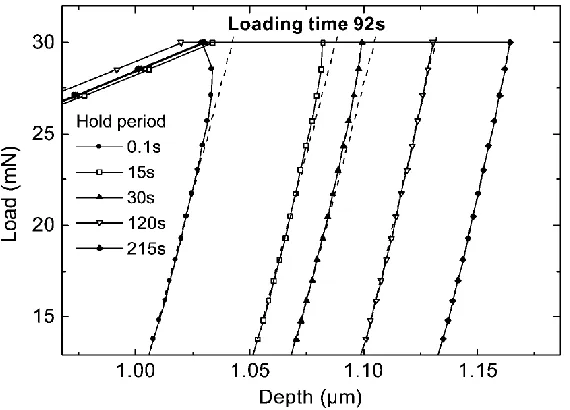
A maximum load of 10 mN is applied by increasing the normal load from 0 mN to 10 mN in 30 seconds and bringing it back to zero at the same rate. Hold period of 187 seconds is chosen for the aluminum alloy to minimize the creep effects during the unloading part of the curve [24]. Figure 3.8 shows the normal load vs time curve of the indentation procedure. The Al 1100 sample was diamond turned to get a surface finish of 15 nm Ra which is less than 5% of the maximum indentation depth, and, thus satisfying the roughness requirement for nanoindentation.

(60)

37 The values of Young’s modulus calculated are shown in Table 3.2 with the mean and standard deviation. These values are close to Young’s modulus value obtained from the tensile test of Al 1100 samples as shown in Figure 3.19.

Table 3.2. Young’s modulus values from the four indentation tests with mean and the standard deviation calculated.

Indent 1 Indent 2 Indent 3 Indent 4 Mean Standard

deviation

Young’s

modulus

(GPa)

78.466146 72.662752 65.795585 80.247657 74.293035 5.0651036581

(61)

38 (a) (b)

Figure 3.9. Scanning probe microscopy (SPM) images of nano indents.

(62)

39 Figure 3.11. Set 2 indents-force vs displacement curve with measured reduced modulus values of Al 1100.

In order to identify the coefficient of friction between the indenter tip and sample surface, Nano-scratch tests were performed. The amount of friction will affect the pile-up height of the indent as seen in section 2.1.4. A schematic representation of the nano-scratch test operation is shown in Figure 3.12. A typical scratch test consists of three stages: the pre-scan stage, the scratch stage, and the post-scan stage. The pre-scan stage is used to measure the surface under the lowest possible normal force around 4 μN so that no permanent damage is made on the surface. In his stage, the tip is moved laterally by 5 μm in one direction. In the scratch stage, the normal force is increased to 1 mN and the tip is moved laterally in the opposite direction by 10

(63)

40 ratio of lateral force and normal force as shown in Figure 3.14 will be used in the finite element models.

Figure 3.12. Schematic diagram of the general operation of the nano-scratch tester when taking a scratch measurement.

(64)

41 Figure 3.14. Time history plot of the ratio of lateral force and normal force on the indenter tip during the nano-scratch test.

3.2.2. Nanoindentation test on glassy carbon

Four indents were made on a glassy carbon sample at the locations shown by four green circles in Figure 3.17 (a) and the loading rate, unloading rate and the hold period of the indentation procedure is shown in Figure 3.15. The force-displacement curves were obtained as shown in Figure 3.16. The reduced modulus values derived from the experiment are converted to Young’s modulus values by using Equation 3.4 and are found to be 30-31 GPa. Scanning probe microscope (SPM) images of the glassy carbon surface before and after the indentation are shown in Figure 3.17 (b).

(65)

42 should be visible in the SPM image. However, the unloading curve doesn’t return to zero displacement and indent impressions are visible as shown in Figure 3.17 (b) respectively. This indicates that the glassy carbon sample did not behave as a pure linear elastic material and there was some plastic deformation.

(66)

43 Figure 3.16. Force vs displacement curve with measured reduced modulus values of glassy carbon.

(a) (b)

(67)

44 3.3. Correlation of FEA models with nanoindentation experiments

3.3.1. Finite element model of the nanoindentation on Al 1100

For the finite element modeling, AbaqusTM _{commercial software was used. Abaqus/Explicit} which implements the explicit solution method to solve the model was used for this simulation as it solves contact problems with greater ease as compared to implicit procedure. Since a quasi-static process is, by definition, a long-time solution, it is often computationally expensive to simulate an event in its natural time scale. The advantage of using Abaqus/Explicit is that the event can be accelerated while keeping inertial forces very low leading to faster solution times [19].

(68)

45 Figure 3.18. Schematic representation of the finite element model of the rigid axisymmetric indenter and mold specimen for nanoindentation using Berkovich indenter.

The indenter was meshed with RAX2 elements: 2 node linear axisymmetric rigid link elements and the mold specimen was meshed with CAX4R elements: 4 node bilinear axisymmetric quadrilateral, reduced integration, hourglass control elements. A finer mesh near the indenter tip and a coarser mesh away from the indenter tip was used for the mold specimen as shown in Figure 3.20. The non-linear geometry option was used in the finite element simulation. Arbitrary Lagrangian Eulerian (ALE) adaptive mesh domain was defined for the mold specimen as it involved large deformations. The nodes on the axis of symmetry were applied with the X symmetry boundary condition by restraining the degrees of freedom: U1, UR2 and UR3. The bottom surface of the mold was completely fixed. The creep observed during the hold period in the experiments is not modeled.

(69)

46 performed and Figure 3.19 shows the average true stress versus true strain curve. The Young’s modulus was measured to be 75.773 GPa with a yield stress of 114.1 GPa. Isotropic hardening material behavior was employed to model the plasticity region of the material.

Figure 3.19. True stress versus true strain curve obtained from the tensile test of Al 1100 H14.

The force-displacement curve obtained from the simulation were compared with the experimental curves as shown in Figure 3.21. The displacement of the node just below the sharp tip and the reaction force on the indenter is depicted in this plot. With the indenter modeled as a sharp tip, the curves are significantly different.

(70)

47 Figure 3.21. Comparison of force vs displacement curves obtained from the experiments and the simulation.

(71)

48 Figure 3.22. Comparison of force vs displacement curves obtained from the experiments and the simulations.

(72)

49 Al 1100 material properties used in the nano-indentation simulation. Figure 3.25 shows the comparison of force vs displacement curves obtained from the experiments and the simulations. The higher yield stress of 140 MPa could be because of the material behaving stiffer in compression.

Table 3.3. Material properties of Al 1100 used in the simulation.

Density Young’s modulus Poisson’s

ratio

Yield stress Tangent modulus

2710 kg/m3 _{75.7736 GPa} _0.33 _{140 MPa} _{0.5 GPa}

Figure 3.23. Height contour image of the Berkovich Indenter scanned under the Keyence confocal microscope.

(a) (b)

(73)

50 Figure 3.25. Comparison of force vs displacement curves obtained from the experiments and the simulation.

(74)

51 (a) (b)

Figure 3.26. Z contour plot of the experimental and simulation nano indents using the Berkovich indenter. (a) Experimental contour plot (b) Simulation contour plot.

Figure 3.27. Error plot of experiment and simulation indent profiles.

3.3.2. Finite element model of the nanoindentation on glassy carbon

(75)

52 modeled as a perfectly linear elastic material. The force vs displacement curve comparison of the experiment and simulation don’t match as shown in Figure 3.28.

Figure 3.28. Comparison of force vs displacement curves obtained from the experiments and the simulation.

(76)

53 Figure 3.29. Von Mises stress distribution of the glassy carbon mold specimen at the end of the loading period of the simulation.

Table 3.4. Material properties of glassy carbon extracted from the nanoindentation experiments.

Young’s modulus Poisson’s ratio

30 GPa 0.2753

3.4. Conclusion

(77)

(78)

55

4. CORRELATION OF INDENTATION EXPERIMENTS AND FINITE ELEMENT

SIMULATIONS USING A 2X2 DIE

4.1. Indentation experiments using 2x2 die

A 2x2 die was fabricated using Focussed Ion Beam (FIB) milling technique. Figure 4.1 shows the 2x2 die scanned under the Keyence VKX1100 laser confocal microscope provided by the Analytical Instrumentation Facility (AIF) at North Carolina State University. The distance between adjacent features (pitch) is around 25 μm and the radius of curvature of each feature is

approximately 15.84 μm. Indentation experiments were conducted using a 2x2 die on an Al 1100 mold. Figure 4.2 shows the experimental setup used for the indentation experiments. The Al 1100 mold is a circular disc, diamond turned to a suitable roughness. The die with the 2x2 features is held in the die holder. The optical probe to measure the indentation depth is connected to the right of the die holder and points towards the mold specimen. This ensures that any machine compliance is not captured in the displacement measured by the probe. The micro-height adjuster is used to adjust the location of the die in the Y direction. The reaction force on the die is measured using a piezoelectric load cell installed behind the die holder. Five indents to a depth of 8.2 μm were made at enough distance from each other. The force vs displacement curves

(79)

56 Figure 4.1. Contour image of the 2x2 die scanned under the Keyence VKX1100 confocal microscope. Approximate radius of each feature ≈ 15.84 μm. Distance between the center of each feature = 25.0164 μm.

(80)

57 Figure 4.3. Force vs displacement curves measured by the optical probe for the 2x2 die indentation.

(a) (b) (c)

(81)

58 4.2. Correlation of FEA simulations using a 2x2 die and indentation experiments

4.2.1. Finite element model setup

For the finite element modeling, AbaqusTM _{commercial software was used. Abaqus/Explicit} which implements the explicit solution method to solve the model was used for this simulation as it solves contact problems with greater ease as compared to implicit procedure. Since a quasi-static process is, by definition, a long-time solution, it is often computationally expensive to simulate an event in its natural time scale. The advantage of using Abaqus/Explicit is that the event can be accelerated while keeping inertial forces very low leading to faster solution times [19].

(82)

59 model the die. Isotropic hardening material behavior was employed to model the plasticity region of the mold material. As Abaqus / Explicit solver was used for the analysis, a load step and an unload step time of 1.2 e-5 seconds was employed. Mass scaling with a factor of 1000 was used to artificially decrease the computational time needed for the simulation. The bottom of the mold was fixed. The loading rate and the mass scaling value chosen were suitable enough to ensure that the kinetic energy was always below 5% of the internal energy of the whole model during the simulation, thus satisfying the conditions for the simulation to remain quasi-static. An indent depth of 8.2 μm was used as obtained from the force vs displacement curves in Figure 4.3. Penalty based friction formulation was employed as the interaction between the die surface and the mold surface in simulations. Friction co-efficient values ranging from 0.1 to 0.4 were used to get a range of force vs displacement curves.

(a) (b)

Figure 4.5. Mesh pattern of the 2x2 die and the mold specimen: Die meshed with C3D10M elements and mold specimen meshed with C3D8R elements.

4.2.2. Finite element analysis results

(83)

60 obtained from Figure 4.3. The force vs displacement curve for a friction coefficient of 0.2 matched well with the experimental curve. Figure 4.7(a) and Figure 4.7(b) shows the experimental Z contour plot and the simulation Z contour plot respectively of the 2x2 die indentation. Figure 4.8 shows the error plot of the experiment and simulation contour plot. The error lies in the range of 12% - 14% of maximum indentation depth. The source of this error could be slight misalignment of the simulation and experiment contours before calculating the error plot. The scanned model of the 2x2 die under Keyence confocal laser microscope usually has significant noise which has to be cleaned and smoothed before it can be meshed in Abaqus. The error might also be because of the loss of data of the CAD model during conversion from Keyence data.

(84)

61 (a) (b)

Figure 4.7. (a) Experimental Z contour plot of the 2x2 indent. (b) Simulation Z contour plot of the 2x2 indent.

(85)

62 4.3. Conclusion

(86)

63

5. DEVELOPMENT OF MULTI-FEATURED DIES AND INDENTATION

STRATEGIES

5.1. Preliminary study

To fabricate a mold with millions of lens features on it the indentation process has to be done fast. An indentation rate of 1 KHz will be used to create microlens arrays (3840 x 2160 pixels, 4K resolution) which is a total of 8294400 pixels. Indenting with a die having multiple lens features on it helps to transfer the features on to the mold in a faster and efficient way. The specifications of the desired multi-lens array mold are shown in Figure 5.1. The radius of the spherical lens is 15.84 μm, the pitch is 25 μm and the indent depth is 15.84 μm. A 3x3 die was designed as shown in Figure 5.2. As the features on this die have uniform size, this die will be referred as 3x3 die (U) in the rest of the thesis for convenience. Each hemisphere is of radius 15.84 μm with a pitch of 25 μm and a fillet radius of 5 μm at the intersection of the spheres. The edges in the desired mold have mathematically sharp edges which is not possible to be fabricated due to manufacturing limitations. For the same reason, the die is modelled with filleted edges which also aids in carrying out FEA simulations without causing any element distortion and singularity issues.

(87)

64 Figure 5.2. CAD model of the 3x3 die. Die referred as 3x3 die (U).

(88)

65 Figure 5.3. Plan view explaining the terminologies of column and rows to refer to indent.

Figure 5.4. Preliminary indentation strategies where each square represents one lens feature. The number represents the indent order and the gray represents the current indent. 3x3 die (U) is used for the indentation.

5.1.1. Finite element model setup for the preliminary indentation strategies

(89)

66 A finite element model of the indentation procedure using a 3x3 die was developed. The die was meshed with C3D10M (10 noded tetrahedral quadratic elements) as this is the preferred element to model finite sliding surface to surface contact conditions to get accurate results. The mold specimen was meshed with C3D8R: 3D continuum 8 noded reduced integration elements. Figure 5.5 shows the meshed 3x3 die and mold specimen. The mesh on the mold was made finer in the central region where the indentations would be made as compared to a coarser mesh in the remaining region to save some computational time. Non-linear geometry option was used in the finite element simulation. Arbitrary Lagrangian Eulerian (ALE) adaptive mesh domains was defined for the mold specimen as it involved large deformations. The mold specimen was fixed at the bottom.

Figure 5.5. Mesh pattern of the 3x3 die and the mold specimen: Die meshed with C3D10M elements and Mold specimen meshed with C3D8R elements.