LIU, SHUFANG. Modeling Mean Residual Life Function Using Scale Mixtures. (Under the direction of Dr. Sujit K. Ghosh.)
The mean residual life function (mrlf) of a subject is defined as the expected re-maining (residual) lifetime of the subject given that the subject has survived up to a given time point. It is well known that under mild regularity conditions, an mrlf determines the probability distribution uniquely. Therefore, the mrlf can be used to formulate a statistical model just as it is done with the survival and hazard functions. In practice, the advantage of the mrlf over the more widely used hazard function lies in its interpretation in many applications where the primary goal is often to characterize the remaining life expectancy of a subject instead of the instantaneous failure rate.
In this thesis, we first develop a smooth nonparametric estimator of the mean residual life function based on a set of right censored observations. The proposed smooth estimator is obtained by a scale mixture of the empirical estimate of the mrlf. The large sample properties of the estimator are established. A simulation study shows that the proposed scale mixture mean residual life function is more efficient in terms of having lower mean squared error (MSE) than some of the existing estimators available in the literature. Further, as the scale mixture mean residual life function has a closed analytical form, it is computationally less demanding for data with a very large sample size compared to other smooth estimators of the mrlf. Thus the scale mixture estimator of the mean residual life function turns out to be both statistically and computationally more efficient.
mrlf, such as the proportional mean residual life (PMRL) model and the linear mean residual life (LMRL) model, have limited applications due to ad-hoc restriction on the parameter space. The regression model that we propose does not have any constraint. It turns out that the proposed proportional scaled mean residual life (PSMRL) model is equivalent to the accelerated failure time (AFT) model. We use full likelihood by nonparametrically estimating the baseline mrlf using the smooth scale mixture estimator that we developed earlier. The regression parameters are estimated using an iterative procedure. A simulation study is carried out to assess the properties of the estimates of the regression parameters. We illustrate our regression model by applying it to the well-known Veteran’s Administration lung cancer data.
Scale Mixtures
by Shufang Liu
a dissertation submitted to the graduate faculty of north carolina state university
in partial fulfillment of the requirements for the degree of
doctor of philosophy
statistics
raleigh, north carolina July 10, 2007
approved by:
Dr. Sujit K. Ghosh (Chair) Dr. Dennis D. Boos
I would like to express my deepest gratitude and appreciation to my advisor, Dr. Sujit Ghosh, for his excellent guidance and inspiration. I am deeply impressed by his in-telligence and patience. I will always remember that he told me to think in a broad way about anything. I could not be where I am today without his help and advising. Thank you, Dr. Ghosh.
I would like to thank my other committee members, Dr. Dennis Boos, Dr. Wenbin Lu, and Dr. Daowen Zhang, for providing me with precious advice on revising this thesis.
It has been a very pleasant experience to study in the department. I would like to thank all of the faculty and staff for their help and assistance. In particular, special thanks must go to Dr. Bill Swallow and Adrian Blue for their great help when my visa needed changing. Thanks to the department for providing me financial support.
Thanks to all my fellow students, especially Qianyi Zhang, Hongmei Yang, Joe Boyer, Justin Shows, Xiaohua Gong, Youfang Liu, Amy Nail, Marti Jones, John Schweitzer, Chris Franck, Wook Hwang, Luciano Silva, and Jiezhun Gu for their help and support. I will always remember our ’happy lunch hour’ at Hillsborough office.
List of Tables . . . vii
List of Figures . . . viii
1 Mean Residual Life Function . . . 1
2 Single Sample Analysis Using Scale Mixtures . . . 9
2.1 Introduction . . . 9
2.2 Scale Mixture Mean Residual Life Function . . . 16
2.3 A Simulation Study . . . 25
2.4 Application to a Melanoma Study . . . 29
2.5 Discussion and Future Work . . . 31
3 Regression Analysis Using Scale Mixtures . . . 43
3.1 Introduction . . . 43
3.2 Proportional Scaled Mean Residual Life Model . . . 55
3.3 A Simulation Study . . . 61
3.4 Application to a Lung Cancer Trial . . . 64
4.1 Introduction . . . 70
4.2 Conditional Mean Residual Life Function with Time-dependent Covari-ates . . . 84
4.3 A Simulation Study . . . 87
4.4 Application to the TUMOR Data . . . 92
4.5 Discussion and Future Work . . . 96
Bibliography . . . 101
Appendix . . . 110
A Proof of Feller Approximation Lemma . . . 111
B Details of a Scale Mixture of mˆe(t) to Obtain mˆm(t) . . . 113
C Properties of Weibull Distribution . . . 115
2.1 The scale parameters for the Exponential distribution . . . 26 2.2 Estimated mrlf’s with 95% CI at some time points for the Melanoma
study . . . 30 2.3 Relative biases and efficiencies of estimated mrlf’s under 0% censoring
rate . . . 38 2.4 Relative biases and efficiencies of estimated mrlf’s under 20% censoring
rate . . . 39 2.5 Relative biases and efficiencies of estimated mrlf’s under 40% censoring
rate . . . 40 2.6 Relative biases and efficiencies of estimated mrlf’s under 60% censoring
rate . . . 41 2.7 Relative efficiencies of mmrlf to emrlf for a sample size of 5000 . . . 42
3.1 Results based on the simulation study . . . 63 3.2 Parameter estimates and estimated standard errors based on AFT model
for the lung cancer data . . . 65
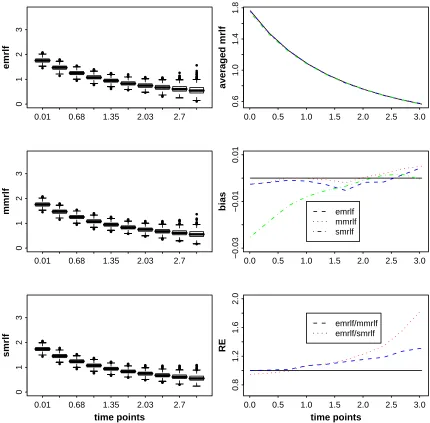
2.1 Estimated mean residual life function for Wei(2, 2) under 0% censoring rate. Panels 1, 3, and 5 are boxplots for emrlf, mmrlf, and smrlf. Panel 2 compares averaged emrlf, averaged mmrlf, and averaged smrlf with the true mrlf. Panel 4 compares biases from averaged emrlf, averaged mmrlf, and averaged smrlf with 0. Panel 6 shows the relative efficiencies of emrlf to mmrlf and emrlf to smrlf. . . 33 2.2 Estimated mean residual life function for Wei(2, 2) under 20% censoring
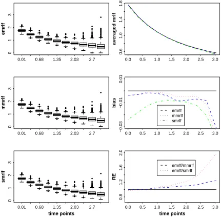
rate. Panels 1, 3, and 5 are boxplots for emrlf, mmrlf, and smrlf. Panel 2 compares averaged emrlf, averaged mmrlf, and averaged smrlf with the true mrlf. Panel 4 compares biases from averaged emrlf, averaged mmrlf, and averaged smrlf with 0. Panel 6 shows the relative efficiencies of emrlf to mmrlf and emrlf to smrlf. . . 34 2.3 Estimated mean residual life function for Wei(2, 2) under 40% censoring
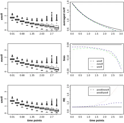
rate. Panels 1, 3, and 5 are boxplots for emrlf, mmrlf, and smrlf. Panel 2 compares averaged emrlf, averaged mmrlf, and averaged smrlf with the true mrlf. Panel 4 compares biases from averaged emrlf, averaged mmrlf, and averaged smrlf with 0. Panel 6 shows the relative efficiencies of emrlf to mmrlf and emrlf to smrlf. . . 36 2.5 Estimated mean residual life function and 95% confidence interval from
case resampling for the Melanoma Study. Panel 1 is emrlf, mmrlf, and smrlf. Panel 2 is emrlf and CI. Panel 3 is mmrlf and CI. Panel 4 is smrlf and CI. . . 37
3.1 Boxplot for results based on the simulation study. Panels 1 and 2 are boxplots forβ1 = 1 andβ2 = 1 from experimentβ = (1,1), respectively. Panels 3 and 4 are boxplots for β1 = 0 and β2 = 1 from experiment
β = (0,1), respectively. ’G’ represents Gehan estimate. ’L’ represents logrank estimate. ’M’ represents estimate from our PSMRL model ap-proach. . . 68 3.2 Comparison of the conditional mean residual life functions for the lung
study with the Monte Carlo sample size of 500. The left boxplot is for the parameterα(true value 1). The middle boxplot is forβ1 (true value -0.5). The right boxplot is for γ (true value 0.5). . . 91 4.2 Kernel density estimate of posterior samples of the regression coefficient
for dose based on using only fixed covariate AFT model for the TUMOR data. . . 98 4.3 Kernel density estimate of posterior samples of the regression coefficient
for dose based on using fixed and time-dependent covariates AFT model for the TUMOR data. . . 99 4.4 Kernel density estimate of posterior samples of the regression coefficient
Mean Residual Life Function
Let T be a positive valued random variable that represents the lifetime of a subject. For example, T could represent the time until a patient dies due to a terminal disease, the time until a piece of equipment fails, or the time until a stock value exceeds or proceeds a given threshold value. Next, let F(t) = Pr[T ≤ t] be the cumulative distribution function (cdf). Notice that F(0) = 0 as T >0 with probability 1.
In survival analysis, it is customary to work with thesurvival function (sf), defined as S(t) = 1−F(t) = Pr[T > t]. For the rest of the development, we assume that T
has finite expectation, i.e., E(T) =R0∞tdF(t) = R0∞S(t)dt <∞.
Definition 1. The mean residual life function (mrlf ) of a lifetime random variable T with finite expectation is defined as
mT(t)≡m(t)≡E[T −t|T > t] =
R∞ t
S(u)
S(t)du, S(t)>0,
0 , otherwise,
(1.1)
where S(t) denotes the survival function associated with T.
From its definition, it is clear that an mrlf gives a measure of the expected remaining (residual) lifetime of a subject given that the subject has survived at least up to time
biomedical studies, reliability models, actuarial sciences and economics, where the goal is often to characterize the residual life expectancy.
A related function that is often used in such studies is known as the hazard func-tion, which is defined as h(t) = −dlogdtS(t) (assuming that the survival function S(t) is differentiable). A hazard function can be equivalently interpreted as the risk of instan-taneous failure of a subject given that the subject has survived up to time t. Notice that
h(t) = lim δ→0
Pr[t < T ≤t+δ|T > t]
δ = limδ→0
S(t)−S(t+δ)
S(t)δ =− S′(t)
S(t),
where S′(t) denotes the first derivative of S(t), assuming that it exists at t >0. Sometimes, in applied sciences, the mean residual life function can serve as a more useful tool than the hazard function, because the mean residual life function has a direct interpretation in terms of average behavior. For example, patients in a clinical trial might be more interested to know how many more years they are expected to survive given that they began a treatment at a certain time ago as compared to their risk of instantaneous dying given that they have started the treatment at a given time (Elandt-Johnson and (Elandt-Johnson, 1980). In an industrial reliability study, researchers prefer the use of the mrlf to that of the hazard function, because they can determine the optimal maintaining and replacing time for a device based on the mrlf (Bhattacharjee, 1982). In economics, Kopperschmidt and Potter (2003) gave an example of applying the mrlf in market research. In the social sciences, Morrison (1978) used an increasing mrlf to model the lifelengths of wars and strikes. A variety of applications of the mean residual life function can be found in Guess and Proschan (1988).
to each other by a one-to-one map, in the sense that one can be obtained from the other provided that they are well-defined, as can be seen by the following lemma:
Lemma 1. Let h(t) be the hazard function of a lifetime random variable T. Then the mrlf m(t) of T is differentiable and is obtained by solving the following differential
equation:
m′(t) + 1 =m(t)h(t) for all t >0,
where m′(t) denotes the first derivative of m(t).
Proof: From (1.1), it follows that m(t)S(t) = Rt∞S(u)du. The result follows by differentiating both sides of the previous identity with respect to (wrt) t and using the definition of h(t). It thus follows that givenh(t) we can obtain
m(t) =
Z ∞ t
exp
−
Z u t
h(θ)dθ
du, (1.2)
and given m(t) we can obtain
h(t) = m
′(t) + 1
m(t) . (1.3)
However, Guess and Proschan (1988) pointed out that it is possible for the mrlf to exist but for the hazard function not to exist (e.g., the standard Cantor ternary function), and also it is possible for the hazard function to exist but for the mrlf not to exist (e.g., S(t) = 1−π2tan−1t).
We know that the mrlf has a wide range of applications. On top of that, the knowledge of the mrlf completely determines the distribution via the inversion formula:
S(t) = m(0)
m(t) exp
−
Z t
0
1
m(u)du
Notice that m(0) =E(T)<∞.
In most applications, data for a given study mainly consist of two types: either all the observations are completely observed or some of the observations are censored. Let
Ti denote the survival time of the ith subject for i= 1, . . . , n. If all the realizations of
{Ti, i= 1, . . . , n}are completely observed, i.e., if the observed data set isD0 ={Ti, i= 1, . . . , n}, then we can easily obtain an estimate of the mrlfm(t) as defined in equation (1.1) either based on a parametric model (e.g., Gamma, Weibull, Log-normal etc.) or nonparametrically as follows:
ˆ
me(t) =
Pn
i=1P(Ti−t)I(Ti−t)
n
i=1I(Ti −t)
, for t∈[0, T(n)), (1.5)
whereI(·) denotes the indicator function, such thatI(u) = 1 ifu >0, otherwiseI(u) = 0. Notice that, ift≥T(n), we define ˆme(t) = 0, whereT(n)= max{Ti, i= 1, . . . , n}. By the strong law of large numbers (SLLN), it follows that ˆme(t) is a consistent estimate of
m(t) and by the Donsker’s Theorem, it follows that√n( ˆme(t)−m(t)) is asymptotically a Gaussian process with mean identically zero and the covariance function given by
σ(s, t) = S(s)1S(t)Rt∞u2dF(u)− 1
S(t)
R∞
t udF(u)
2
, 0≤s≤t <∞ (Yang, 1978). However, in many applications, the Ti’s are often right censored by a random variable. Let Ci denote the censoring time of the ith subject, i.e., we only observe
available in the literature in Section 2.1, which describes methods of estimating m(t) based on a censored data set D1 as defined above. We analyze a real censored data
set from a Melanoma study (Ghorai et al., 1980) in Section 2.4. This data set has 27 uncensored observations and 41 censored observations. The mean residual life function based on this data set is estimated in Section 2.4.
In practice, in addition to just a single sample of iid observations, we might observe a vector of pexplanatory fixed covariates, say denoted by Zi = (Zi1, . . . , Zip)τ for each subject i= 1, . . . , n. The Zi’s are variables which are recorded at the baseline and do not change throughout the treatment period, such as age, gender, initial weight, and so on. We assume that the Zi’s are observed without any measurement errors. In this case, assuming that some responses Ti’s may be right censored randomly by Ci’s, we will observe DR ={(Xi,∆i,Zi), i = 1, . . . , n}, where as before Xi = min{Ti, Ci} and ∆i =I(Ci−Ti). In this case, we assume that for each subject givenZi, theTi’s andCi’s are conditionally independent and the triplets (Ti, Ci,Zi) are also independent across subjects, i = 1, . . . , n. Given a data set DR, our goal is to estimate the conditional mean residual life function (cmrlf ) defined as
m(t|z)≡E[T −t|T > t,Z =z] =
Z ∞ t
S(u|z)
S(t|z)du, (1.6)
where S(t|z) = Pr[T > t|Z =z] denotes the conditional survival function of T given
In survival analysis, besides fixed covariates, we often encounter time-dependent covariates along with the survival time. Time-dependent covariates are variables that are changing throughout the treatment period, such as smoking status, cholesterol level, CD4 count, and so on. For simplicity, we shall assume that there is only one time-dependent covariate in the study, to be denoted by Vi(t) for the ith subject. Let
¯
Vi(t) ={Vi(s); 0≤s≤t}be the history of the covariate process at timet. In practice, it is rare for one to observe the entire sample path ofVi(t), but only at a few time points ti = {tij, j = 1, . . . , mi} of the clinic visits, where timi ≤ Xi, i.e., no measurement is
available after the subject is dead or censored. Hence, the observed data are DB =
{Xi,∆i,Zi,V¯i,ti}for i = 1, . . . , n, where ¯Vi = {Vi(tij), j = 1, . . . , mi}. In this case, we assume that the Ti’s and Ci’s are conditionally independent and (Ti, Ci,Zi,V¯i) are also independent across subjects, i = 1, . . . , n.Given a data set DB, the conditional mean residual life function (cmrlf ) is defined as
m(t|z,v¯(t))≡E[T −t|T > t,Z =z,V¯(t) = ¯v(t)] =
Z ∞ t
S(u|z,v¯(u))
S(t|z,v¯(t))du, (1.7)
where S(t|z,v¯(t)) = Pr[T > t|Z = z,V¯(t) = ¯v(t)] denotes the conditional survival function of T given Z = z and ¯V(t) = ¯v(t). We review some regression models with time-dependent covariates in the literature in Section 4.1, and then analyze a real data set with a time-dependent covariate from a TUMOR study (see Example 54.5 of SAS online documentation) in Section 4.4. This data set has a censoring rate of 44.4%. The data set has a fixed covariate as dose levels and a time-dependent covariate as number of papillomas.
which are proper in the sense that the model corresponds to a function that is based on a valid probability model. However, some cmrlf’s are not proper in the sense that the modeled m(t|z) does not satisfy all the requirements of a function being an mrlf (see Theorem 1). We discuss several available methods to model m(t|z) within the regression set up in Section 3.1. To the best of our knowledge, we have not found regression analysis of the mean residual life function for data with time-dependent covariates.
Before we develop and discuss statistical methods to estimate the mrlfm(t), based on a single sample data D1, the cmrlf m(t|z), based on a data set DR with fixed covariates, or the cmrlf m(t|z,v¯(t)), based on a data set DB with time-dependent covariates, we state a characterization theorem for an mrlf:
Theorem 1. (Hall-Wellner, 1981)
Let m: R+→R+ be a function that satisfies the following conditions:
(i) m(t) is right continuous and m(0) >0;
(ii) e(t)≡m(t) +t is non-decreasing;
(iii) if m(t−) = 0 for some t=t0, then m(t) = 0 on [t0,∞);
(iv) if m(t−)>0 for all t, then R0∞1/m(u)du=∞.
Let ι≡inf{t:m(t−) = 0} ≤ ∞, and define
S(t) = m(0)
m(t) exp
−
Z t
0
1
m(u)du
.
Then F(t) = 1−S(t) is a cdf on R+ with F(0) = 0 and ι = inf{t : F(t) = 1}, finite
Proof: See Hall and Wellner (1981), page 172.
Remark 1. Any mrlf m(t) obviously satisfies the four conditions (i)-(iv) of the above Theorem. In the sequel, an mrlf or cmrlf that violates one of the above four
conditions will be termed as an improper mrlf and we will compare our methods to
only those that are based on proper mrlf ’s (for single sample problems) or cmrlf ’s (for
regression problems).
Single Sample Analysis Using Scale
Mixtures
2.1
Introduction
As we mentioned in Chapter 1, let T be a lifetime random variable. If there is no cen-soring, the data set will be denoted byD0 ={Ti, i= 1, . . . , n}. If there is censoring, let
Ci denote the censoring time of theith subject, i.e., we only observe Xi = min{Ti, Ci} and the indicator of censoring ∆i =I(Ci−Ti) fori= 1, . . . , n. The data set in case of censoring will be denoted by D1 ={(Xi,∆i), i= 1, . . . , n}. It is assumed that (Ti, Ci) are independent and identically distributed (iid) and T is independent of C. The esti-mators of the survival function and the hazard function based on the data sets D0 and
D1 are commonly studied in the literature. Here we summarize some of the research
methods on estimating the mean residual life function based on a complete data set
D0 and a censored data set D1, respectively.
The mean residual life function (mrlf ) of a lifetime random variable T with finite expectation is defined as
m(t)≡E[T −t|T > t] =
R∞ t
S(u)
S(t)du, S(t)>0,
0 , otherwise.
It can be seen from (2.1) that the mrlfm(t) has a disadvantage for its high depen-dence on the tail behavior of the survival function. Therefore, it is hard to estimatem(t) with precision, especially when no parametric form can be specified. If the underlying distribution is assumed to arise from a parametric family, then it will be straightfor-ward to estimatem(t). Tsang and Jardine (1993), Lai et al. (2004) obtained estimates of m(t) based on a 2-parameter Weibull distribution model, while Agarwal and Kalla (1996), Kalla et al. (2001), and Gupta and Lvin (2005) obtained estimates based on a Gamma distribution model. Gupta and Bradley (2003) studied m(t) when the Ti’s were assumed to belong to the Pearson family of distributions. However, it is obvious that the parametric assumptions affect the shape and character of the mrlf which, in case of an incorrect specification, is undesirable, especially when prediction is of in-terest. Many researchers then focus on using nonparametric estimation procedures to study m(t).
Yang (1978) employed the empirical survival function ˆS(t) of S(t) in (2.1) under the assumption of no censoring, which results in a discontinuous estimate of m(t) at each observation. The empirical estimator of m(t) for a complete data set D0 is given
by
ˆ
me(t) =
Z ∞ t
ˆ
S(u) ˆ
S(t)du, (2.2)
wherenSˆ(t) = Pni=1I(Ti−t) is the number of individuals surviving up to timet. The empirical estimator ˆme(t) was shown to be asymptotically unbiased and uniformly strong consistent, and to converge in distribution to a Gaussian process (Yang, 1978). Although ˆme(t) has good asymptotic properties, it is a discontinuous estimate of
There are different approaches to obtain smooth estimators of m(t) in the literature. Essentially, all the methods derive the smooth estimators ofm(t) by smoothing ˆS(·) in (2.2). Some researchers smoothed ˆS(·) by using the kernel density methods, such as the classical kernel density method, the recursive kernel density method, or the classical kernel density method with a local linear fitting technique. Some researchers applied Hille’s theorem (Hille, 1948) to smooth ˆS(·). In this study, we use scale mixture to smooth ˆme(t) directly instead of first obtaining a smooth estimator of S(·).
Kulasekara (1991) used a smoothed estimator of S(·) in the numerator and the denominator in (2.2) for complete and censored data, and presented an estimator of m(t) by constructing a kernel density estimator of the lifetime density. The resulting estimator of m(t) is smooth because of the smoothness of the kernel estimator of the density function. For a complete data set D0, the kernel density estimator off at time
t is given by
fnK(t) = n
X
i=1
1
nhK
t−Ti
h
, t≥0,
whereK is a symmetric kernel density function, andhis the bandwidth,h=h(n)→0 and nh(n)→ ∞ as n→ ∞.
The estimator of the distribution function F(t) corresponding to this density func-tion fK
n (t) is then given by
FK n (t) =
Z t −∞
fK
n (u)du= 1
n
n
X
i=1 W
t−Ti
h
,
whereW(t) =R−∞t K(u)du. It follows that the estimator ofS(t) is given bySK
n (t) = 1−
FK
ˆ
S(·) in (2.2) by its smooth version SK
n (·), which is given by
ˆ
mK(t) =
R∞ t S
K n(u)du
SK n(t)
. (2.3)
Kulasekara (1991) proved the asymptotic consistency and normality of ˆmK(t). The choice of K could be based on the Epanchmikov Kernel (K(t) = 34(1−t2)I(1− |t|)), which is obtained by minimizing C(K) = [R−∞+∞t2K(t)dt]2
5[R+∞
−∞ K
2(t)dt]4
5. Since
dif-ferent K’s do not make a significant impact in terms of C(K), its choice could be arbitrary. Besides considering the degree of differentiability and computational feasi-bility, the most important issue is how to select a desired bandwidth h. Most often the choice of his based on some cross-validation criteria. In the simulation study, Ku-lasekera (1991) demonstrated that the kernel estimator of the mrlf can be significantly improved by judicious choice of a certain bandwidth. Moreover, the kernel estimator was shown to often have much smaller mean squared error (MSE) than the empirical estimator based on a simulation study. Consequently, the kernel estimator ˆmK(t) is more efficient compared to the empirical estimator ˆme(t).
Ruiz and Guillamon (1996) replaced the empirical survival function in the numer-ator by a recursive kernel estimate and kept the empirical survival function in the de-nominator in (2.2). To reduce the bias of the basic kernel density estimator, Swanepoel and Graan (2005) introduced a new kernel density function estimator based on a non-parametric transformation of complete data. Abdous and Berred (2005) adopted the classical kernel smoothing method to estimate m(t) for complete data using a local linear fitting technique.
the empirical survival functions both in the numerator and the denominator in (2.2) only for complete data. For an ordered sample with no ties (T(1), . . . , T(n)) of size n,
the empirical survival function Sn is defined by
Sn(t) = n−k
n forT(k)≤t < T(k+1), k = 0,1, . . . , n. (2.4)
Define a set of nonnegative weights as
wk(tλn) = e−tλn(tλn)
k
k! , k = 0,1,2, . . . ,∞,
whereλn = Tn(n) is chosen to be data-dependent, which makes the weight functionwk(·) stochastic. Hence, the smoothed survival function can be obtained as
˜
Sn(t) = X k≥0
Sn
k λn
wk(tλn).
Plugging the smoothed survival function into (2.2), the smooth estimator of m(t) is given by
˜
mn(t) = 1
λn
Pn k=0
Pk
r=0((tλn)(k−r)/(k−r)!)Sn(k/λn)
Pn
k=0((tλn)k/k!)Sn(k/λn)
. (2.5)
Chaubey and Sen (1999) proved that ˜mn(t) is a consistent estimator of m(t) and
λ1n/2( ˜mn(t)−m(t))→d N
0,mS((tt))pointwise.
alive at the end of the period of study. Therefore, estimating the mrlf based on right censored data is necessary.
Ghorai et al. (1980) first used the Bayes estimator of S(t) into (2.1) to obtain the estimate of m(t) under the assumption of right censoring. The empirical estimator of
m(t) for a censored data set D1 is given by
ˆ
me(t) =
RM
t Sˆn(u)du ˆ
Sn(t) , (2.6)
where M =M(n)→ ∞, and
ˆ
Sn(t) = N
+(t) + 1 n+ 1
n
Y
j=1
2 +N+(Xj) 1 +N+(X
j)
[∆j=0,Xj≤t]
, (2.7)
whereN+(t) = Pn
i=1I(Xi−t) denotes the number of censored and uncensored subjects surviving up to t. The asymptotic consistency and normality of ˆme(t) were proved by Ghorai et al. (1980).
of f at time t is given by
fnK(t) = n
X
i=1
1
haiK
t−Xi
h
, t≥0,
where ai is the size of jump at Xi and it is 0 if ∆i = 0, i.e., when Xi is censored. The size of jump ai can be estimated by ˆSi−Sˆi+1, where ˆSi =Qi−j=11
n−j n−j+1
∆j
. The estimator of the distribution functionF(t) corresponding to this density functionfK
n (t) is given by
FnK(t) =
Z t −∞
fnK(u)du= n
X
i=1 aiW
t−Xi
h
,
where W(t) = R−∞t K(u)du. Then, the smooth estimator of S(t) is given by SK n (t) = 1−FK
n (t). Therefore, the smooth estimator ˆmK(t) of m(t) for censored data can be obtained by substituting ˆSn(t) by its smooth version SK
n (t) into (2.6), which is given by
ˆ
mK(t) =
R∞ t S
K n(u)du
SK n(t)
. (2.8)
In this study, we also extend the estimation procedures for m(t) of Chaubey and Sen (1999) for complete data to censored data. We utilize the Kaplan-Meier estimator of S(·) for censored data in (2.5), instead of the empirical survival function from (2.4) for complete data. In the simulation study (Section 2.3), the behavior of the estimator from the extension is compared with that of our smooth estimator.
residual life function. The mixture mrlf is defined as
mF(t) =
R∞
t SF(u)du
SF(t) =
R∞ t
R∞
0 S(u, θ)π(θ)dθdu
R∞
0 S(t, θ)π(θ)dθ
=
Z ∞
0
m(t, θ)π(θ|t)dθ, (2.9)
where m(t, θ) =
R∞
t S(u,θ)du
S(t,θ) and π(θ|t) =
π(θ)S(t,θ)
R∞
0 S(t,θ)π(θ)dθ. Finkelstein stated that the
mixture mrlf mF(t) could be studied by knowing S(t, θ). However, S(t, θ) is usually unknown. This mixture mrlf is again based on a mixture of the survival function as opposed to a direct mixture of the mrlf.
Besides a lot of studies about estimating m(t), there are many studies about testing the mrlf in the literature, for instance, Hollander and Proschan (1975), Berger et al. (1988), Ahmad (1992), and Ahmed and Alwasel (2003).
In Section 2.2, we propose a smooth estimator ofm(t) using scale mixture and then examine the asymptotic properties of the proposed mrlf. In Section 2.3, we present a simulation study to evaluate the performances of the proposed mrlf. In Section 2.4, we compare the performance of the empirical mrlf, the smooth mrlf (Chauby and Sen, 1999), and our proposed mrlf based on a real data set. In Section 2.5, we present some discussion and directions for further extensions.
2.2
Scale Mixture Mean Residual Life Function
smooth estimator ˆmm(t) will be called the scale mixture mean residual life function. We then present closed analytical expressions for ˆme(t) and ˆmm(t) for complete and right censored data. Finally, we provide the asymptotic properties of ˆmm(t).
First, we restate the result due to Petrone and Veronese (2002) based on Feller (1966, p.219).
Lemma 2. Feller Approximation Lemma:
Let g(·) be a bounded and right continuous function on R for each t. Let Zj(t) be a sequence of random variables for each t such that µj(t) ≡ E[Zj(t)] → t and σ2j(t) ≡
V ar[Zj(t)]→0 as j → ∞. Then
E[g(Zj(t))]→g(t) ∀t.
The proof of the lemma is given in Appendix A. Now, we introduce the Scale Mixture Theorem.
Theorem 2. Scale Mixture Theorem: Let m(t) = E[T −t|T > t] be an mrlf. Then
(a) m(θtθ) is a proper mrlf for any θ >0;
(b) R0∞m(θtθ)π(θ)dθ is a proper mrlf for any density π(·) on (0,∞).
Proof: Notice that, for θ >0,
m(tθ)
θ = E[T −tθ|T > tθ]
1
θ
= E
T θ −t
Tθ > t
Hence, m(θtθ) is the mrlf of Tθ and (a) is proved. Next,
Z ∞
0
m(tθ)
θ π(θ)dθ = Eπ
E
T θ −t
Tθ > t
θ = E T θ −t
Tθ > t
Hence, R0∞ m(θtθ)π(θ)dθ is the mrlf of Tθ where Tθ|θ ∼ m(θtθ) and θ ∼ π(·), and (b) is proved. Notice that the mrlf uniquely determines a distribution from the inversion formula (1.4), thus T
θ|θ ∼ m(tθ)
θ , which means that the conditional distribution of T
θ given θ is the distribution induced by m(θtθ).
Remark 2. Notice that the above result is valid even when T is discrete-valued.
From Theorem 1, we can see that ˆme(t) is a right continuous function on [0, T(n)]
and ˆme(t) = 0 for t > T(n) and hence, ˆme(t) is a bounded function. Then, we can use
the Feller Approximation Lemma to approximate ˆme(t). Let Zn(t)∼ Ga
kn,ktn
for
t > 0, where kn is a function of n, kn→ ∞ as n→ ∞. Ga
kn,ktn
denotes a Gamma distribution with mean µn(t) =t and variance σ2
n(t) = t
2
kn, and the density function is
given by
fkn,t(z) =f
z
kn,
t kn = kn t kn 1 Γ(kn)z
We propose the following as a scale mixture estimator of m(t):
ˆ
mm(t) = E[ ˆme(Zn(t))] =
Z ∞
0
ˆ
me(u)f
u
kn,
t kn du = Z ∞ 0 ˆ
me(u)
kn
t
kn
1 Γ(kn)
ukn−1e−knut du let θ= u t = Z ∞ 0 ˆ
me(tθ)
θ π(θ|kn)dθ, (2.10)
where π(θ|kn) = kknn
Γ(kn)θkne−knθ is the density function of Ga
kn+ 1,k1n
, and hence it follows from (b) of the Scale Mixture Theorem (Theorem 2) that ˆmm(t) is a scale mixture mean residual life function and it is a proper mrlf.
The closed analytical form of ˆme(t) for complete data is given in (1.5). Here we present a unified closed analytical form of ˆme(t) for complete and censored data. Let the ordered observed data be 0 def= X0 < X1 < . . . < Xn < Xn+1
def
= ∞, assuming no ties. Then ˆme(t) can be expressed as
ˆ
me(t) =
Pn
j=1(Xj−t)I(Xj−t)wj
Pn
j=1I(Xj−t)wj , 0< t≤Xn,
0 , t > Xn,
= Pn
j=l+1Xjwj
Pn
j=l+1wj −t, Xl ≤t < Xl+1, l = 0,1, . . . , n−1,
0 , t > Xn,
(2.11)
where the weight function is wj =Fn(Xj)−Fn(Xj−), andFn(Xj) is the Kaplan-Meier (KM) estimate. Notice that wj = 1n for complete data.
censored data based on (2.10). The details of a scale mixture of ˆme(t) to obtain ˆmm(t) are given in Appendix B. The closed analytical form for ˆmm(t) is given by
ˆ
mm(t) = Z ∞
0
ˆ
me(u)f
u
kn,
t kn
du
≈ nX−1
l=0
Pn
j=l+1Xjwj Pn
j=l+1wj
F
Xl+1
kn,
t kn −F Xl kn,
t kn −tF Xn kn+ 1,
t kn
,(2.12)
where F ·kn,ktn
is the cdf of Gakn,ktn
.
Remark 3. If Fn(Xj) in the weight function wj is the KM estimate for data with tied observations, mˆe(t) and mˆm(t) based on data with tied observations can be calcu-lated using the same closed forms as (2.11, 2.12).
Next we show that ˆmm(t) is a smooth mrlf. The following set of sufficient conditions guarantees that ˆmm(t) is a smooth estimator of m(t) for a general weight function
π(θ|kn) in (2.10), which needs not be a Gamma density function. The conditions are
(A1) π(θ|kn) is a smooth density on (0,∞), such that R0∞1
θπ(θ|kn)dθ < ∞ for all n and
(A2) If Yn∼πn(·|kn), then Yn P
→1 as n → ∞.
In this study, π(θ|kn) is chosen to be the density function of Gakn+ 1,k1n
, such that Z ∞ 0 1
θπ(θ|kn)dθ =
Z ∞
0
1
θ kkn
n Γ(kn)θ
kne−knθ = 1,
and hence condition (A1) is satisfied. Also whenYn ∼Ga
kn+ 1,k1n
, it follows that
E[Yn] = kn+ 1
kn
= 1 + 1
kn →
and
V ar[Yn] =
kn+ 1
k2
n
= kn+ 1
kn 1
kn →
0 as n → ∞,
and hence condition (A2) is satisfied. Therefore, our scale mixture mean residual life function ˆmm(t) is a smooth estimator.
Finally, we provide the asymptotic properties of ˆmm(t) in the following Theorem:
Theorem 3. We assume that kn in Ga
kn+ 1,k1n
satisfies kn = cn1+ǫ where
ǫ > 0 and c >0 is a known constant. Consider the estimator mˆm(t) defined in (2.10) that satisfies the conditions (A1) and (A2). Then,
(i) mˆm(t) pointwisely converges in probability to m(t).
(ii) √n( ˆmm(t)−m(t)) is asymptotically a Gaussian process with mean identically zero and the covariance function σ(s, t), where
σ(s, t) = 1
S(s)S(t)
Z ∞ t
u2dF(u)− 1
S(t)
Z ∞ t
udF(u)
2
, 0≤s≤t <∞
for complete data and
σ(s, t) = 1
S(s)S(t)
Z ∞ t
φ2(ν)
(S(ν)G(ν))2dHe(ν), 0≤s≤t <∞,
where φ(t) = Rt∞S(u)du, G(t) = Pr[C > t], and He(t) = Pr[∆1 = 1, X1 ≤ t] for
censored data.
Using the results of Yang (1978) for complete data and Ghorai et al. (1980) for censored data, we have the following asymptotic properties for the empirical estimator
ˆ
(a) ˆme(t) pointwisely converges in probability to m(t). In other words,
lim
n→∞P(|mˆe(t)−m(t)| ≥ǫ) = 0 for ǫ >0.
(b) √n( ˆme(t)−m(t)) is asymptotically a Gaussian process with mean identically zero and the covariance function given by σ(s, t).
In order to prove (i) and (ii) of Theorem 3, it is sufficient to show that√n|mˆm(t)− ˆ
me(t)|→P 0 as n → ∞.
Proof:
Since ˆme(t) pointwisely converges in probability to m(t) from Yang (1978) and Ghorai et al. (1980), i.e.,
ˆ
me(t)→P m(t) as n→ ∞
and
Yn P
→1 as n→ ∞,
then by the Slutsky’s Theorem
ˆ
me(tYn)
Yn P
→ m(t∗1)
1 =m(t).
Notice that mˆe(YtYn)
n is the mrlf of ˜
Tn
Yn, where ˜Tn takes on the values of T1, . . . , Tn each
with probability 1n. Then we can see that EhT˜n
Yn −t
T˜n
Yn > t, Yn
i
can obtain the following relationship by the Dominated Convergence Theorem
E
ˆ
me(tYn)
Yn
P
→E[m(t)] wrt π,
i.e.,
ˆ
mm(t)→P m(t).
This completes the proof of (i) of Theorem 3.
Now we prove (ii) of Theorem 3. Notice that
√
n( ˆmm(t)−m(t)) =√n( ˆmm(t)−mˆe(t)) +√n( ˆme(t)−m(t)),
where √n( ˆme(t)−m(t))∼GP(0, σ(·,·)).
If we can prove that√n( ˆmm(t)−mˆe(t))→P 0 asn→ ∞, (ii) of Theorem 3 is proved. Now we consider √n( ˆmm(t)−mˆe(t)) = √nEhmˆe(YtYn)
n −mˆe(t)
i
. First, we take Taylor’s expansion of mˆe(YtYn)
n aroundt, which is given by
ˆ
me(tYn)
Yn
= mˆe(t)
Yn
+(tYn−t) ˆm ′ e(t∗n)
Yn
,
where t∗ n
P
→ t as n → ∞. It can be seen from (2.11) that ˆme(t) is differentiable iff
t ∈(Xl, Xl+1), l= 1, . . . , n−1 and ˆme(t) is not differentiable if t=Xl, l= 1, . . . , n−1. Thus, ˆm′
Second, we substitute the Taylor’s expansion into√nEhmˆe(YtYn)
n −mˆe(t)
i
, i.e.,
√
n( ˆmm(t)−mˆe(t)) = √nE
ˆ
me(tYn)
Yn −
ˆ
me(t)
= √nE
ˆ
me(t)
Yn −
ˆ
me(t) + (tYn−t) ˆm ′ e(t∗n)
Yn = E √ n 1
Yn − 1
ˆ
me(t)−√n
1
Yn − 1
tmˆ′e(t∗n)
If we can prove√nY1 n −1
P
→0 asn → ∞, then we can obtain√n( ˆmm(t)−mˆe(t))→P 0 as n→ ∞ and the proof is complete. SinceYn∼Ga
kn+ 1,k1n
, then E √ n 1
Yn − 1
=√n
E 1 Yn −1
=√n
kn
kn+ 1−1 − 1 = 0 and V ar √ n 1
Yn − 1
=n∗V ar
1
Yn
=n k
2
n
k2
n(kn−1)
= n
kn−1
.
Since we assume kn = cn1+ǫ where ǫ > 0 and c is a constant, it can be seen that
V arh√nY1 n −1
i
→ 0 as n → ∞. Therefore, √nY1 n −1
P
→ 0 as n → ∞ is
proved. Hence, this completes the proof of Theorem 3.
Remark4. Notice that the asymptotic properties ofmˆm(t)are the same as those of the estimator of Yang (1978) for complete data and the same as those of the estimator
2.3
A Simulation Study
It is difficult to obtain the exact mean squared error (MSE) of the scale mixture mean residual life function. We conducted a simulation study to explore the properties of the estimator. We extended the smooth estimation procedures of Chaubey and Sen (1999), which were originally developed for only complete data, to censored data. The simula-tion study was used to compare the performances of the empirical mrlf ˆme(t) (emrlf), the scale mixture mrlf ˆmm(t)(mmrlf), and the smooth mrlf ˆms(t) (smrlf)(Chaubey and Sen, 1999).
The simulation study was carried out under the following conditions:
• The true distribution is Weibull distribution. The properties of Weibull distribution are listed in Appendix C. The data are generated from Wei(2, 2), where the shape parameter and the scale parameter are both 2. The performances of emrlf, smrlf, and mmrlf are evaluated at the time points from quantile 0.01 to quantile 0.90 of this distribution.
• The censoring distribution is Exponential distribution with the scale pa-rameter λ. The choices of λ to obtain the average censoring rates of 0%, 20%, 40%, and 60% are listed in Table 2.1.
• A sample size of n = 100 and a Monte Carlo sample size of N = 1000 are used in the simulation study.
• The tuning parameter kn in the Gamma distribution of the scale mixture mrlf ˆmm(t) (mmrlf) is set to kn=n1.01.
• The bias can be estimated by ˆB(t) = PNi=1mˆi(t)
estimated by M SE\(t) = 1
N−1
PN
i=1( ˆmi(t)−m¯ˆ(t))2+B(t)2. The relative ef-ficiency can be estimated by RE12d (t) = M SE\1(t)
\
M SE2(t). In this study, \
M SEemrlf(t)
\
M SEmmrlf(t)
,
\
M SEemrlf(t)
\
M SEsmrlf(t), and
\
M SEsmrlf(t)
\
M SEmmrlf(t) are compared.
Table 2.1: The scale parameters for the Exponential distribution
Average Censoring Rate λ
0% ∞
20% 7.6
40% 3.2
60% 1.7
Figures 2.1-2.4 show the graphical summary of the simulation for the targeted censoring rates of 0%, 20%, 40%, and 60%, respectively. In each figure, Panels 1, 3, and 5 feature the boxplots of the 1000 repetitions of ˆm(t) changing with time for emrlf, mmrlf, and smrlf, respectively. Panel 2 compares the averaged emrlf, mmrlf, and smrlf from the 1000 repetitions with the true mrlf. Panel 4 compares the bias of averaged emrlf, mmrlf, and smrlf with 0. Panel 6 shows the relative efficiencies (RE) of emrlf to mmrlf (in dotted line) and emrlf to smrlf (in dash line). Tables 2.3-2.6 list the relative biases and the relative efficiencies for the experiments of the censoring rates of 0%, 20%, 40%, and 60%, respectively.
because the information provided by the data is limited by the censored observations. Figure 2.1 and Table 2.3 present the simulation results for data with 0% censoring rate, i.e., complete data. We have the following key findings:
(i) It can be seen from Figure 2.1 that emrlf, mmrlf, and smrlf have similar performances for the small and moderate time points.
(ii) It can be observed from Figure 2.1 that emrlf has the largest variation and the smrlf has the least variation for the extreme time points.
(iii) From Table 2.3, it can be seen that smrlf has larger relative biases at small time points compared to emrlf and mmrlf. It turns out that these biases of smrlf are statistically significant (P-value<0.05) for all time points smaller than 1.92 (the 33th percentile of this Weibull distribution).
(iv) Generally, mmrlf has smaller biases than emrlf, though none of the biases of emrlf or mmrlf are significantly different from 0.
(v) In terms of efficiency, mmrlf is always better than emrlf. The smrlf is less efficient for small time points and more efficient for large time points compared to emrlf and smrlf.
smrlf for complete data.
Figure 2.2 and Table 2.4 present the simulation results for data with 20% censoring rate (small). We get similar results for slightly censored data as for the complete data; i.e., mmrlf is a better estimator compared to emrlf and a better estimator for small data points compared to smrlf.
Figure 2.3 and Table 2.5 present the simulation results for data with 40% censoring rate (moderate). For all the time points studied in this simulation, smrlf is significantly biased. It appears that emrlf and mmrlf are only biased for time points larger than the 87.5th percentile of the Weibull distribution (P-value < 0.05). Therefore, for moderately censored data, mmrlf is a better estimator compared to emrlf and smrlf.
Figure 2.4 and Table 2.6 present the simulation results for data with 60% censoring rate (extreme). For highly censored data, emrlf, mmrlf and smrlf are all significantly biased for all the time points evaluated (P-value < 0.05). However, the biases from emrlf and mmrlf are smaller than those from smrlf. Therefore, for highly censored data, emrlf, smrlf and mmrlf are not so good estimators for a moderate sample size (n=100). However, given the fact that all these estimators are asymptotically unbiased, the biases eventually vanish with an increasing sample size.
have closed analytical forms, it did not take much time to do the simulation for emrlf and mmrlf. Table 2.7 lists the relative efficiencies of emrlf to mmrlf for the censoring rate of 0%, 20%, 40%, and 60%. It can be seen that mmrlf is a more efficient estimator of the mrlf compared to emrlf for data with a very large sample size.
2.4
Application to a Melanoma Study
We applied our estimation method to the data set given in Ghorai et al. (1980) to obtain mmrlf. We also computed the empirical mrlf estimator (emrlf) and the modified Chaubey and Sen’s estimator (smrlf) for this data set. This data set has 68 observations, which are listed below, corresponding to the survival time (in weeks) of 68 participants of a Melanoma study conducted by the Central Oncology Group with headquarters at the University of Wisconsin-Madison. This data set has a high censoring rate of 58.8%.
Uncensored observations: 16, 44, 55, 67, 73, 76, 80, 81, 86, 93, 100, 108, 114, 120,
125, 129, 134, 140, 147, 148, 151, 152, 181, 190, 193, 213, 215.
Censored observations: 13, 14, 19, 20, 21, 23, 25, 26, 27, 31, 32, 34, 37, 38, 40, 46,
50, 53, 54, 57, 57, 59, 60, 65, 66, 70, 85, 90, 98, 102, 103, 110, 118, 124, 130, 136,
138, 141, 194, 234.
estimator, mmrlf and smrlf are smooth estimators. It also can be seen that emrlf vanishes at the largest time point, while mmrlf and smrlf can still take positive values. This indicates that mmrlf and smrlf can have a better prediction performance than emrlf even outside the observed time range.
Table 2.2: Estimated mrlf’s with 95% CI at some time points for the Melanoma study
time 23.4 58.5 117 175.5 210.6
emrlf 120.8 89.4 53.2 31.2 10.1
(97.1, 139.5) (75.3, 108.1) (38.8, 71.8) (21.6, 50.8) (1.9, 30.8)
mmrlf 120.8 89.1 54.2 32.2 15.5
(105.6, 139.3) (74.3, 107.2) (40.6, 69.8) (23.9, 45.0) (8.8, 24.5)
smrlf 118.6 88.4 55.0 33.6 21.9
(101.5, 137.1) (71.9, 105.8) (39.3, 70.2) (21.8, 44.3) (11.8, 28.3)
Notice that the conclusions derived from Table 2.2 can not be made using the hazard function directly. This illustrates one of the advantages of using the mean residual life function over the traditional hazard function.
2.5
Discussion and Future Work
In the literature, researchers usually use (2.2) to calculate the empirical mrlf ˆme(t); i.e., they often first estimate the survival function and then calculate ˆme(t). The closed analytical form of ˆme(t) from (2.11) provides an easy and unified calculation procedure for complete data and right censored data. The closed form of our scale mixture mean residual life function ˆmm(t) from (2.12) can be used to obtain a nonparametric smooth estimator of the mrlf for complete and right censored data.
From the simulation studies presented in Section 2.3, it follows that ˆmm(t) is always a better estimator compared to ˆme(t). In terms of bias, ˆmm(t) is always a better esti-mator compared to the modified Chaubey and Sen’s (1999) estiesti-mator ˆms(t). In terms of MSE, ˆmm(t) is competitive to ˆms(t). Finally, ˆme(t) and ˆmm(t) are computationally less demanding compared to ˆms(t).
For moderately censored data, our scale mixture mean residual life function ˆmm(t) performs reasonably well for the smaller time points, while the modified Chaubey and Sen’s estimator ˆms(t) performs better for the larger time points. It may be worth combining these two estimators using a weight function as follows:
ˆ
where w(t) is a suitable weight function that is a decreasing function of t. Although we have not explored this option, it might be a good research topic as part of a future study.
An alternative estimator can be obtained by using a version of restricted splines. Let 0 =t0 < t1 < t2 < . . . < tm < tm+1 =∞ be a partition of [0,∞). Define
mj(t) = aj(tj−t)+, j = 1, . . . , m,
where aj ∈ (0,1) and x+ = x if x ≥ 0, otherwise x+ = 0. It can be proved that
mj(t), j = 1, . . . , mbelong to Hall-Weller family (Theorem 1). Therefore, a finite mixture of mrlf’s can be defined as
mf(t) = n
X
j=1
wjmj(t), n
X
j=1
wj = 1, wj ≥0.
0.01 0.68 1.35 2.03 2.7
0
1
2
3
emrlf
0.0 0.5 1.0 1.5 2.0 2.5 3.0
0.6
1.0
1.4
1.8
averaged mrlf
0.01 0.68 1.35 2.03 2.7
0
1
2
3
mmrlf
0.0 0.5 1.0 1.5 2.0 2.5 3.0
−0.03
−0.01
0.01
bias emrlf
mmrlf smrlf
0.01 0.68 1.35 2.03 2.7
0
1
2
3
time points
smrlf
0.0 0.5 1.0 1.5 2.0 2.5 3.0
0.8
1.2
1.6
2.0
time points
RE
emrlf/mmrlf emrlf/smrlf
0.01 0.68 1.35 2.03 2.7
0
1
2
3
emrlf
0.0 0.5 1.0 1.5 2.0 2.5 3.0
0.6
1.0
1.4
1.8
averaged mrlf
0.01 0.68 1.35 2.03 2.7
0
1
2
3
mmrlf
0.0 0.5 1.0 1.5 2.0 2.5 3.0
−0.03
−0.01
0.01
bias
emrlf mmrlf smrlf
0.01 0.68 1.35 2.03 2.7
0
1
2
3
time points
smrlf
0.0 0.5 1.0 1.5 2.0 2.5 3.0
0.8
1.2
1.6
2.0
time points
RE
emrlf/mmrlf emrlf/smrlf
0.01 0.68 1.35 2.03 2.7
0
1
2
3
emrlf
0.0 0.5 1.0 1.5 2.0 2.5 3.0
0.6
1.0
1.4
1.8
averaged mrlf
0.01 0.68 1.35 2.03 2.7
0
1
2
3
mmrlf
0.0 0.5 1.0 1.5 2.0 2.5 3.0
−0.20
−0.10
0.00
bias emrlf
mmrlf smrlf
0.01 0.68 1.35 2.03 2.7
0
1
2
3
time points
smrlf
0.0 0.5 1.0 1.5 2.0 2.5 3.0
0.8
1.2
1.6
2.0
time points
RE
emrlf/mmrlf emrlf/smrlf
50 100 150 200
0
20
40
60
80
100
120
mrlf
emrlf mmrlf smrlf
50 100 150 200
0
20
40
60
80
100
120
emrlf
50 100 150 200
20
40
60
80
100
120
time points
mmrlf
50 100 150 200
20
40
60
80
100
120
time points
smrlf
Table 2.3: Relative biases and efficiencies of estimated mrlf’s under 0% censoring rate
time Bbemrlf(t)
m(t)
b
Bmmrlf(t)
m(t)
b
Bsmrlf(t)
m(t)
\
M SEemrlf(t)
\
M SEmmrlf(t)
\
M SEemrlf(t)
\
M SEsmrlf(t)
\
M SEsmrlf(t)
\
M SEmmrlf(t)
0.010 -0.001 -0.001 -0.014 1.000 0.947 1.056
0.169 -0.002 -0.001 -0.014 1.003 0.961 1.044
0.328 -0.001 -0.001 -0.013 1.014 0.970 1.045
0.488 -0.001 -0.001 -0.011 1.015 0.992 1.024
0.647 -0.001 0.000 -0.010 1.012 0.987 1.025
0.806 -0.001 0.000 -0.009 1.037 1.021 1.015
0.965 -0.001 0.000 -0.008 1.056 1.056 1.000
1.124 -0.002 0.000 -0.007 1.067 1.069 0.998
1.284 -0.001 0.000 -0.006 1.064 1.067 0.997
1.443 -0.004 -0.001 -0.005 1.096 1.099 0.998
1.602 -0.004 -0.002 -0.005 1.091 1.102 0.990
1.761 -0.004 -0.002 -0.004 1.159 1.198 0.967
1.920 -0.004 -0.001 -0.002 1.162 1.226 0.948
2.080 -0.002 0.001 -0.001 1.155 1.244 0.928
2.239 0.001 0.002 0.001 1.182 1.309 0.903
2.398 -0.003 0.003 0.002 1.186 1.354 0.876
2.557 -0.001 0.005 0.003 1.261 1.490 0.846
2.716 0.000 0.007 0.003 1.248 1.541 0.810
2.876 0.008 0.009 0.001 1.256 1.643 0.765
3.035 0.008 0.009 -0.001 1.312 1.852 0.708
Table 2.4: Relative biases and efficiencies of estimated mrlf’s under 20% censoring rate
time Bbemrlf(t)
m(t)
b
Bmmrlf(t)
m(t)
b
Bsmrlf(t)
m(t)
\
M SEemrlf(t)
\
M SEmmrlf(t)
\
M SEemrlf(t)
\
M SEsmrlf(t)
\
M SEsmrlf(t)
\
M SEmmrlf(t)
0.010 -0.001 -0.001 -0.013 1.000 0.966 1.036
0.169 -0.001 -0.001 -0.013 1.002 0.977 1.026
0.328 -0.001 -0.001 -0.012 1.010 0.981 1.030
0.488 0.000 0.000 -0.010 1.013 1.007 1.006
0.647 0.000 0.001 -0.009 1.010 1.002 1.008
0.806 0.000 0.001 -0.007 1.035 1.038 0.998
0.965 0.000 0.001 -0.006 1.052 1.067 0.986
1.124 -0.001 0.001 -0.005 1.057 1.077 0.981
1.284 0.001 0.001 -0.005 1.063 1.084 0.981
1.443 -0.001 0.001 -0.004 1.083 1.105 0.980
1.602 -0.002 -0.001 -0.004 1.083 1.117 0.969
1.761 -0.005 -0.002 -0.004 1.124 1.187 0.947
1.920 -0.005 -0.002 -0.004 1.152 1.240 0.929
2.080 -0.005 -0.001 -0.004 1.143 1.253 0.912
2.239 -0.002 0.000 -0.004 1.160 1.308 0.887
2.398 -0.006 0.000 -0.004 1.177 1.374 0.857
2.557 -0.002 0.002 -0.005 1.222 1.486 0.822
2.716 -0.005 0.003 -0.008 1.178 1.517 0.777
2.876 0.002 0.003 -0.012 1.237 1.722 0.718
3.035 0.000 -0.002 -0.018 1.292 1.963 0.658
Table 2.5: Relative biases and efficiencies of estimated mrlf’s under 40% censoring rate
time Bbemrlf(t)
m(t)
b
Bmmrlf(t)
m(t)
b
Bsmrlf(t)
m(t)
\
M SEemrlf(t)
\
M SEmmrlf(t)
\
M SEemrlf(t)
\
M SEsmrlf(t)
\
M SEsmrlf(t)
\
M SEmmrlf(t)
0.010 -0.002 -0.002 -0.014 1.000 0.977 1.024
0.169 -0.002 -0.002 -0.013 1.004 0.990 1.014
0.328 -0.002 -0.002 -0.012 1.006 0.986 1.020
0.488 -0.002 -0.001 -0.011 1.014 1.013 1.001
0.647 -0.002 -0.001 -0.010 1.004 1.001 1.002
0.806 -0.002 -0.001 -0.009 1.021 1.025 0.996
0.965 -0.002 -0.001 -0.008 1.040 1.061 0.980
1.124 -0.004 -0.001 -0.008 1.047 1.077 0.973
1.284 -0.002 -0.002 -0.008 1.060 1.091 0.971
1.443 -0.004 -0.003 -0.009 1.070 1.110 0.964
1.602 -0.006 -0.005 -0.010 1.069 1.126 0.949
1.761 -0.009 -0.007 -0.011 1.110 1.193 0.930
1.920 -0.010 -0.007 -0.012 1.107 1.212 0.913
2.080 -0.009 -0.006 -0.013 1.113 1.246 0.893
2.239 -0.008 -0.006 -0.015 1.161 1.346 0.862
2.398 -0.011 -0.007 -0.019 1.104 1.345 0.820
2.557 -0.009 -0.011 -0.025 1.171 1.515 0.773
2.716 -0.019 -0.020 -0.034 1.178 1.623 0.726
2.876 -0.028 -0.038 -0.049 1.160 1.712 0.678
3.035 -0.055 -0.070 -0.071 1.243 1.977 0.628
Table 2.6: Relative biases and efficiencies of estimated mrlf’s under 60% censoring rate
time Bbemrlf(t)
m(t)
b
Bmmrlf(t)
m(t)
b
Bsmrlf(t)
m(t)
\
M SEemrlf(t)
\
M SEmmrlf(t)
\
M SEemrlf(t)
\
M SEsmrlf(t)
\
M SEsmrlf(t)
\
M SEmmrlf(t)
0.010 -0.010 -0.010 -0.020 1.000 0.974 1.027
0.169 -0.010 -0.010 -0.021 1.003 0.980 1.023
0.328 -0.011 -0.011 -0.021 1.007 0.986 1.022
0.488 -0.011 -0.011 -0.020 1.010 0.988 1.023
0.647 -0.013 -0.012 -0.021 1.005 0.987 1.018
0.806 -0.014 -0.013 -0.022 1.022 1.014 1.008
0.965 -0.017 -0.016 -0.024 1.020 1.026 0.994
1.124 -0.022 -0.019 -0.027 1.043 1.063 0.981
1.284 -0.023 -0.022 -0.030 1.046 1.073 0.975
1.443 -0.028 -0.026 -0.034 1.030 1.074 0.959
1.602 -0.033 -0.031 -0.039 1.092 1.174 0.930
1.761 -0.039 -0.037 -0.046 1.088 1.201 0.906
1.920 -0.047 -0.044 -0.054 1.095 1.242 0.882
2.080 -0.055 -0.052 -0.065 1.102 1.300 0.848
2.239 -0.058 -0.065 -0.081 1.114 1.394 0.799
2.398 -0.081 -0.087 -0.102 1.132 1.531 0.739
2.557 -0.110 -0.124 -0.131 1.162 1.711 0.680
2.716 -0.155 -0.176 -0.168 1.206 1.921 0.628
2.876 -0.233 -0.246 -0.213 1.196 2.066 0.579
3.035 -0.332 -0.329 -0.266 1.203 2.295 0.524
Table 2.7: Relative efficiencies of mmrlf to emrlf for a sample size of 5000
\
M SEemrlf(t)/M SE\mmrlf(t) censoring rate
time 0% 20% 40% 60%
Regression Analysis Using Scale Mixtures
3.1
Introduction
In Chapter 2, we studied nonparametric estimation procedures of the mean residual life function based on a single sample of iid observations, which are either partially censored or completely observed. However, in many applications, in addition to just a single sample of iid observations, we might observe a vector of p explanatory fixed variables, say denoted by Zi = (Zi1, . . . , Zip)τ for each subjecti= 1, . . . , n.For instance, Zi are the prognostic factors for theith subject andZi1 = treatment,Zi2 = gender,Zi3 = age,
and so on. We assume that theZi’s are observed without any measurement errors. Let
Tidenote the survival time of theith subject fori= 1, . . . , n. We assume that someTi’s may be right censored randomly by Ci’s, and we will observe DR ={(Xi,∆i,Zi), i = 1, . . . , n}, where Xi = min{Ti, Ci} and ∆i = I(Ci −Ti) as before. In this case, we assume that for each subject given Zi, the Ti’s andCi’s are conditionally independent and the triplets (Ti, Ci,Zi) are also independent across subjects, i= 1, . . . , n.
To measure the effect of fixed covariates on the survival time, the proportional hazards model (Cox, 1972) and the accelerated failure time model (Kalbfleisch and Prentice, 1980) are often used. The proportional hazards (PH) model is defined as
where h(·|z) denotes the conditional hazard function of the lifetime random variable
T given Z = z, h0(·) denotes the baseline hazard function, γ denotes the vector
of regression parameters, and the superscript τ denotes the transpose of a vector. Usually, the maximum partial likelihood method is used to estimate and make inference aboutγ. For example, Tsiatis (1981) rigorously proved the consistency and asymptotic normality of the partial likelihood estimate ˆγ. Bagdonavicius (1999) modified the partial likelihood to study the generalized proportional hazards model.
The accelerated failure time (AFT) model is given by
logT =zτβ+e, (3.2)
or
S(t|z) = S0(texp{−zτβ}),
where β is the vector of regression parameters, e = log(T0) where T0 is the baseline
survival time, and S0(·) denotes the baseline survival function. A lot of research has
been done on the AFT model. For example, Miller (1976), Buckly and James (1979), and Lai and Ying (1991) investigated the least squares based and M-estimation method for the AFT model. Tsiatis (1990), Wei et al. (1990), and Ying (1993) used the rank-based method to study the estimation and inference for the regression parameters. Ghosh and Ghosal (2006) approached the statistical inference using a nonparametric Bayesian method.
of a lifetime random variable T with finite expectation is defined as
m(t)≡E[T −t|T > t] =
R∞ t
S(u)
S(t)du, S(t)>0,
0 , otherwise.
(3.3)
To evaluate the effect of fixed covariates on the remaining life expectancy, the conditional mean residual life function has to be studied. The conditional mean residual life function (cmrlf ) is defined as
m(t|z)≡E[T −t|T > t,Z =z] =
Z ∞ t
S(u|z)
S(t|z)du, (3.4)
where m(t|z) is the conditional mean residual life function associated with Z, and
S(t|z) = Pr[T > t|Z =z] denotes the conditional survival function of T given Z =z. Conversely, the conditional survival function can be expressed in terms of the cmrlf as follows:
S(t|z) = Pr(T ≥t,Z =z) = m(0|z)
m(t|z) exp
−
Z t
0
1
m(u|z)du
. (3.5)
Oakes and Dasu (1990) proposed a semiparametric model called the proportional mean residual life (PMRL) model, which is similar to the proportional hazards model,
for studying the association between the mean residual life and the fixed covariates Z. The PMRL model is defined as
m(t|z) = m0(t) exp{g(z,β)}, (3.6)
unspecified and can be interpreted as the mean residual life function for the population of subjects withZ = 0,βis associated regression parameter for covariatesZ =z, andg
is a regression function, such thatg(0,β) = g(z,0) = 0 is satisfied. Usually, researchers take the regression function asg(z,β) = zτβ. In this study, unless specified, g(z,β) =
zτβis used. The PMRL model directly describes the distribution of remaining lifetime and holds appealing interpretation in life expectancy. However, this model has some limitations. One constraint is that e0(t) = m0(t) + t must be nondecreasing (see Theorem 1). Furthermore, another constraint is that m(t|z) should be a proper mrlf for all β. From the two constraints, we can see that
(1) for an increasing baseline mrlf m0(t), m(t|z) is a proper mrlf for all β;
(2) for a decreasing or non-monotonic baseline mrlf m0(t), m(t|z) is a proper mrlf for all β only when it satisfies exp{zτβ}>1.
Thus, in order to obtain a proper estimator of the cmrlf, these two constraints have to be checked after obtaining ˆβ and ˆm0(t). Oakes and Dasu (1990) pointed out that
m(t|z) is an mrlf for all β if m0(t) itself is monotonically nondecreasing, when they
proposed the PMRL model.
Nanda et al. (2006) showed that the proportional mean residual life model leads to the following model in terms of the hazard function
h(t|z) = exp{−zτβ}
1 + exp{zτβ}m′
0(t)
1 +m′
0(t)
h0(t), (3.7)
where m′
0(t) = dm0(t)/dt. It can be seen from (3.7) that β must satisfy the
condi-tion 1 + exp{zτβ}m′
exp{zτβ}>1, which verifies the second constraint we mentioned above. Notice that if
Z >0 then exp{zτβ} →0 as β→ −∞ and if Z <0 then exp{zτβ} →0 as β→ ∞. Thus, exp{zτβ}>1 can not be satisfied for all β.
There is a relationship between the proportional mean residual life function and the proportional hazards function. The hazard function h(·|z) of the forward recurrence time in the renewal processes formed by the T’s is the reciprocal of the mean residual life function m(·|z) (Maguluri and Zhang, 1994). Furthermore, when a model satisfies the assumptions for both the proportional hazards model and the proportional mean residual life model, its underlying distribution belongs to the Hall-Wellner class of distributions with linear mean residual life functions (Oakes and Dasu, 1990). For example, Pareto, Exponential, and a certain class of rescaled Beta distributions have linear mean residual life functions, i.e., m(t) = at+b where b > 0 and a > −1. For
a > 0, a = 0, and −1 < a < 0, the distributions correspond to Pareto distributions, Exponential distributions, and rescaled Beta distributions, respectively.
Chen et al. (2004) pointed out that the proportional mean residual life model and the accelerated failure time model coincide if and only if the baseline mean residual life function m0(t) is constant, i.e., the underlying distribution belongs to the Exponential
family.