ABSTRACT
KUPCHELLA, RYAN LLOYD. Modeling the Evolution of Mesoscale Morphology in C/SiC Ceramic Matrix Composites. (Under the direction of Paul Cooper.)
A mathematical theory and accompanying numerical schemes are developed for pre-dicting the coupled interaction between gas kinetics and material behavior during the CVI process for ceramic matrix composite structures (CMCs) and during the oxidation process for C/SiC CMCs. On the continuum level, gas kinetics are dealt with using theory derived from a form of the mass conservation law for ideal gases in a porous solid. Gas concentrations are obtained by making use of the Bubnov-Galerkin finite element method and are calculated assuming quasi-static evolution that is driven by changes in the structural morphology of the material.
Modeling the Evolution of Mesoscale Morphology in C/SiC Ceramic Matrix Composites
by
Ryan L. Kupchella
A thesis submitted to the Graduate Faculty of North Carolina State University
in partial fulfillment of the requirements for the Degree of
Master of Science
Mechanical Engineering
Raleigh, North Carolina 2011
APPROVED BY:
Dr. Robert Tolson Dr. Fred DeJarnette
Biography
Acknowledgements
The mathematical theory and numerical methods described here are a result of one and a half years of investigation. I would not have reached this point without the support and guidance provided by Dr. Paul Cooper and Dr. Robert Tolson.
Table of Contents
List of Tables . . . vii
List of Figures . . . viii
List of Symbols . . . xi
Chapter 1 Introduction . . . 1
1.1 Mechanisms for Morphology Evolution . . . 3
1.2 Research Goals . . . 4
1.3 Methodology . . . 5
Chapter 2 Fundamentals of Continuum Level Gas Kinetics . . . 7
2.1 Governing Equations . . . 8
2.2 Finite Element Formulation . . . 12
Chapter 3 CVI Process Modeling . . . 15
3.1 State of the Art . . . 15
3.2.1 Governing Equations . . . 17
3.2.2 Model Parameters . . . 18
3.2.3 Finite Element Formulation . . . 21
3.2.4 Verification Solutions . . . 22
3.3 Mesoscale Formulation . . . 23
3.3.1 Level Set Formulation . . . 26
3.3.2 Isolated Pore Detection Algorithm . . . 34
3.3.3 Porosity and Surface Area . . . 42
3.3.4 Verification Solutions . . . 43
3.4 Multi-scale Solution Approach . . . 50
3.5 Processing Examples . . . 53
3.5.1 Image Segmentation and Diffusivity Approximation . . . 54
3.5.2 Refinement Study . . . 57
3.5.3 Final Processing Results . . . 64
Chapter 4 Oxidation Modeling . . . 72
4.1 State of the Art . . . 72
4.2 Continuum Level Formulation . . . 77
4.2.1 Governing Equations . . . 77
4.2.2 Model Parameters . . . 79
4.2.3 Finite Element Formulation . . . 81
4.3 Mesoscale Formulation . . . 86
4.3.1 Fiber Geometry . . . 87
4.3.2 Porosity and Surface Area . . . 88
4.4 Multi-scale Solution Approach . . . 90
4.5 Oxidation Examples . . . 90
Chapter 5 Concluding Remarks . . . 97
List of Tables
Table 3.1 Initial model parameters used with a model refinement study . . . 57
Table 3.2 Model parameters used for final results . . . 64
Table 4.1 Model parameters used for comparison with test data . . . 91
Table 4.2 Model parameters used for the results shown in Figure 4.6 . . . 94
List of Figures
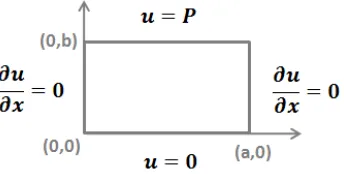
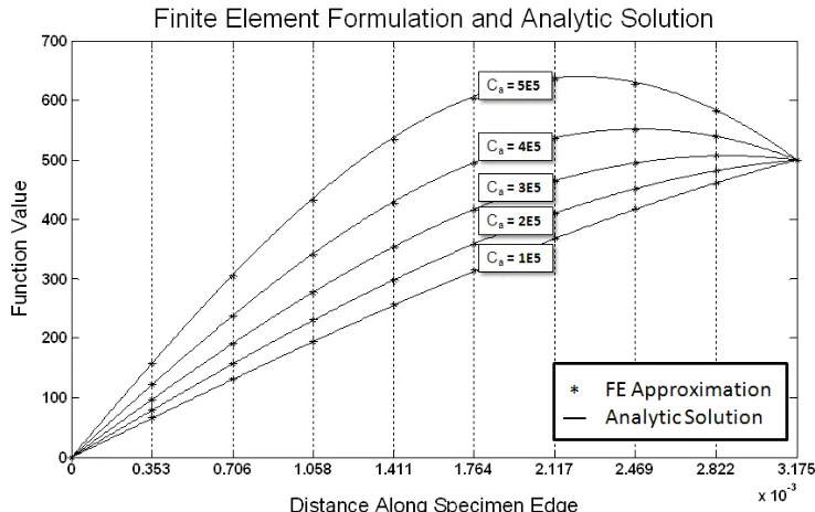
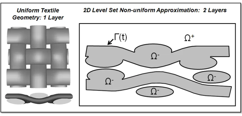
Figure 3.1 Boundary conditions for finite element verification solution . . . . 24 Figure 3.2 Numeric results for finite element verification solution . . . 25 Figure 3.3 Analytical comparison with numeric results for finite element
veri-fication solution . . . 25 Figure 3.4 A physical interpretation of the level set domain . . . 29 Figure 3.5 Example of a level set representation of a small portion of a larger
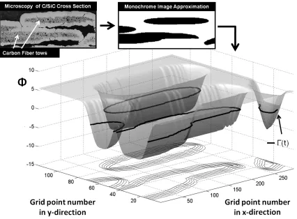
cross section . . . 31 Figure 3.6 Visual representation of the derivative selection process for the
ENO scheme . . . 33 Figure 3.7 Outline of the pore isolation algorithm . . . 36 Figure 3.8 Pictorial representation of assumptions used to model pore isolation
in two dimensions . . . 40 Figure 3.9 Schematic of porosity approximation for an exemplary single cell . 43 Figure 3.10 Visual results of a numerical experiment using different grids . . . 44 Figure 3.11 Results from a numerical experiment using the level set and pore
Figure 3.12 Interpretation of small details on a coarse grid . . . 47
Figure 3.13 Cusp region in Figure 3.10 for three different grids . . . 49
Figure 3.14 Close up of area outlined in Figure 3.10 with boundaries for the previous time step . . . 50
Figure 3.15 Outline of the interface between the continuum level and mesoscale simulations . . . 51
Figure 3.16 Model output and segmented specimen cross section . . . 56
Figure 3.17 Growth around the longitudinal and transverse tows with isolated pores . . . 59
Figure 3.18 Variation in final specimen porosity and model runtimes with re-spect to grid resolution for two Courant numbers . . . 61
Figure 3.19 Variation in final specimen porosity and model runtimes with re-spect to Courant number for two levels of grid resolution . . . 65
Figure 3.20 Variation in final specimen porosity and model runtimes with re-spect to finite element time step for two Courant numbers . . . 66
Figure 3.21 Model output using new model refinement parameters and a seg-mented specimen cross section . . . 67
Figure 3.22 Model output for two processing conditions . . . 68
Figure 3.23 Model output and a CT scan of an actual specimen . . . 70
Figure 3.24 Model output on top of CT scan of an actual specimen . . . 71
Figure 4.2 Contour plots showing the oxygen concentration distribution for two Sherwood numbers after one hour of exposure. . . 76 Figure 4.3 Carbon remaining for fully transient and quasi-steady state analyses 85 Figure 4.4 Partial pressure at a central node for fully transient and
quasi-steady state analyses . . . 86 Figure 4.5 Demonstration of circular fiber bundle approximation . . . 89 Figure 4.6 Weight loss versus time from previous results[6], current model
using the values in Table 4.2, and test data . . . 92 Figure 4.7 Weight loss versus time from previous results[6], current model
List of Symbols
Acronyms
Abbreviation Definition
CMC Ceramic matrix composite; a general class of high performance materials
C/SiC A ceramic matrix composite with carbon fiber reinforcements in a silicon carbide matrix
MTS Methyltrichlorosilane (CH3SiCl3); CVI reactant vapor
SiC/SiC A ceramic matrix composite with silicon carbide reinforcements in a silicon carbide matrix
Multi-scale Variables
Symbol Definition
Sa available surface area per volume
Ψ finite element propagation speed
� effective porosity
Continuum Level Variables
Symbol Definition
k measured reaction rate
p total pressure
pi partial pressure of species i
pi,m nodal partial pressure of species i pe
i elemental partial pressure
ptest partial pressure of reactant during test
dt finite element update frequency
vc volume fraction carbon
vc0 initial volume fraction of carbon i
vm volume fraction of matrix material
xi volume fraction of species i
A pre-exponential factor used in the Arrhenius equation
DAB diffusivity of species A intoB
Def f effective diffusivity
De elemental domain
Ea, Eapp activation energy used in the Arrhenius equation
Ji mass flux of species i
Ks reaction constant used to define the Sherwood number L characteristic length used to define the Sherwood number
Mi molar mass of species i
Nm nodal interpolation function
R universal gas constant
Ri local rate of change of species i per time Ri,m nodal rate of change of species i per time Re
i elemental rate of change of species i per time
Sh Sherwood number
T absolute temperature
Tb boiling point
Tc critical temperature
Vc critical volume
Wn weight function
�/κ Lennard-Jones parameter
λi stoichiometric constant for species i
µg gas viscosity
ρi density of species i
˜
ρc intrinsic density of carbon
˜
ρSiC intrinsic density of SiC
τ system tortuosity
τ0 initial tortuosity
ϕ second-order permeability tensor
∆T contribution to Tc in the Joback method
∆V contribution to Vc in the Joback method
Γe element boundary
Mesoscale Variables
Symbol Definition
n unit vector normal to Γ
p collection of grid points in Ωc
u concentration variable used to detect Ωc
xij grid point on in the level set domain, Ω
xΓ position of a point on Γ
F front propagation speed
α arbitrary direction in the level set domain Ω ϑ collection of grid points with potential to be in Ωc
ν Courant number for the CFL condition
φ level set function
β frequently changing version of ϑ
Γ front or physical boundary between solid and gas Λij array representation of a monochrome image
Ω level set domain
Ω+ collection of regions in Ω where φ >0
Ω− collection of regions in Ω where φ <0 Ωc collection of regions in Ω+ that are isolated
Ωo collection of regions in Ω+ that are not isolated Ωp collection of regions in ΩS located in pores ΩT level set domain containing only transverse fibers ΩL level set domain containing only longitudinal fibers
ΩS superposition of ΩT and ΩL
Chapter 1
Introduction
systems and decreases design complexity.[1, 2, 3]
However, hypersonic and other high temperature aerospace applications typically involve exposure to high temperature oxygen, and manufacturing components capable of resisting strength degradation in such environments presents a significant challenge. Chemical vapor infiltration (CVI) has become a primary means of manufacturing CMC components and has several advantages over alternate production methods such as hot pressing, polymer impregnation and pyrolysis, or reactive melt infiltration. As the name suggests, fabrication is accomplished by infiltrating a preform with a reactant gas such as methyltrichlorosilane (MTS) and a catalyst such as Hydrogen. The preform is a woven network of reinforcing fiber bundles that can have one of a variety of different weave patterns. The gas precursor forms a solid coating around the fibers that accumulates both within and around the fiber bundles. Fiber integrity can be better preserved during CVI because the temperatures and pressures involved are relatively low. Milder temperatures also result in less shrinkage, making near net-shape fabrication more feasible, and a lack of sintering aids mean fewer impurities in the matrix material.[4, 5]
normal to the fiber axis in the final SiC matrix and seal coat during cool down due to the thermal expansion mismatch between the carbon fiber and the silicon carbide matrix. The carbon fiber bundles, or tows, have anisotropic thermal expansion properties and the coefficient of thermal expansion ranges from −0.1×10⁻⁶ to −1.1× 10⁻⁶ /◦C in the longitudinal direction and 7× 10⁻⁶ /◦C in the radial direction; whereas, the SiC matrix material is assumed to behave isotropically with a coefficient of expansion around 4.8×10⁻⁶ /◦C.[3]
The resulting network of micro-cracks and pores in the SiC matrix provides pathways for the ingress of oxygen into the material. The load bearing carbon fibers used in C/SiC CMCs are prone to degradation in oxygen at temperatures beyond 450◦C (840◦F), leading to a loss of strength and ultimately failure of the component. Although coatings can provide some protection from high temperature oxygen, crack opening and oxidation kinetics are functions of several variables, and the interplay between them can cripple coating effectiveness under dynamic conditions.[1, 3] Therefore, modeling the CVI process is not only critical in predicting the strength and elastic properties of a component, it is an important step in understanding the subsequent oxidation of the carbon fiber reinforcements.
1.1
Mechanisms for Morphology Evolution
mechanisms for the evolution of the pore morphology. Throughout the CVI process, CMCs are densified as matrix material is deposited, causing a time dependent decrease in porosity. Contrastingly, the loss of solid material during the oxidation process causes a time dependent increase in porosity.
Both processes can be described by reaction-diffusion equations driven by simple chemical reactions,[5, 6] and the solution of these equations is coupled to the development of porosity. Chemical reactions dictate the rate of porosity formation, and porosity and reaction surface availability effect both the gas diffusion and the chemical reaction rates. When transient boundary conditions are imposed, the gas dynamics involved oc-cur much more quickly than changes in the material structure posing stiff differential equations. However, the CVI manufacturing process and oxidation testing of sample specimens both take place in controlled environments, so for simplicity, only steady state boundary conditions will be considered. In this case, the governing equations become quasi-static.
1.2
Research Goals
be better understood and predicted. Also, life prediction of CMC components could not be made without an understanding of the mechanisms behind the oxidation of load bear-ing carbon fiber reinforcements. Therefore, the objective of this research is to provide a step toward developing techniques for realistically predicting the manufacture of CMC components and the subsequent degradation of carbon fibers in C/SiC CMCs due to oxidation.
1.3
Methodology
The CVI and oxidation processes will be analyzed using two-dimensional simulations. These will test the capability of the methods used and provide the groundwork for creating three-dimensional simulations in the future. The reaction-diffusion equations will be solved using a quasi-static finite element formulation, and the material will be treated as a homogeneous porous media through which oxygen flows. The reactants and the gaseous by-products of each reaction will be assumed to exist in the pores of the material and to obey the ideal gas law.
Chapter 2
Fundamentals of Continuum Level
Gas Kinetics
2.1
Governing Equations
In order to track the change in concentration (or mass) of each type of gas or ”gas species” during the deposition or degradation processes, the mass continuity equation for gases in porous media is incorporated with transport mechanisms for diffusion. In previous work, the mass continuity equation is expressed in terms of species concentration and gases are assumed to behave ideally.[3, 5, 6]
Under the ideal gas assumption, gas species concentrations are directly related to partial pressures. For instance, species concentrations measured in terms of molarity are expressed in units of moles per volume, and species partial pressure for a species i can be calculated simply using a form of the ideal gas law, pi =ciRT whereci is the species molarity, T is the absolute temperature, and R is the universal gas constant. For con-sistency with previous work on oxidation modeling,[6] concentrations will be quantified using partial pressures throughout this paper. The total pressure of a gas mixture can be obtained by summing the partial pressure contributions from each species as follows:
p=
#of species�
i=1
pi (2.1)
The mass continuity equation for gas in a porous media can be written as follows: ∂�ρi
∂t +∇ ·Ji =Ri (2.2)
The chemical reactions are assumed to be first-order reactions, meaning the reaction rates are linear functions of the local reactant concentration.[4, 5, 6, 7] The local reaction rate for the model is calculated as follows:
Ri =−Ki
�
preactant ptest
�
(2.3)
In (2.3), i refers to a particular gas species, preactant is the local partial pressure of the reactant gas during the simulation, and ptest is the partial pressure of the reactant gas present during the test used to measure the reaction rate, k. The value of k can be measured in different ways and may be normalized by an area or a volume. For the processes in this work, k is obtained by a measurement of the change in solid mass per time due to the reaction. The measured rate of gas species production or consumption, Ki, is in units of mass per volume per time and is a function of k that will be defined separately for each process depending on howk is measured.
Ki =f(k) (2.4)
The sign convention will be chosen such that Ki is positive when the species ’i’ is con-sumed and negative when it is produced.
Generally, reaction rates, k, are calculated for various temperatures by making use of an Arrhenius rate equation:[4, 5, 6]
k =Ae−Ea/RT (2.5)
Turning now to the second term on the left hand side of (2.2), the mass flux of a gas in a porous system can be described by the expression:
Ji =−ρDef f∇
�
ρi ρ
�
−ρi 1
µgϕ· ∇p (2.6)
where p is the total pressure of the gas mixture, ρ is the total gas density, and ρi is the density of each species.[6]
The first term in (2.6) is a simplified version of Fick’s first law of diffusion and represents the mass flux of one gas species into another due to concentration gradients. The effective mass diffusivity Def f is in units of area per time.
Def f = �
τDAB (2.7a)
τ = τ0�0
� (2.7b)
where DAB is the Fickian mass diffusion of species A into B, given by Bird,et al.[8] and is derived from Chapman-Enskog theory. In the above, � refers to the effective porosity, τ refers to the tortuosity, and �0 and τ0 refer to initial values of each.[4, 5] Since the
internal structure evolves during the CVI and oxidation processes, the value of Def f will change throughout the simulation as described in section 3.3. This definition ofDef f can be augmented to incorporate the effect of Knudsen diffusion that occurs at scales smaller than the mesoscale.[5, 7]
per length per time and ϕ is a second-order permeability tensor for the solid matrix in units of length squared.[6, 9]
Using the ideal gas law for both the mixture (ρ=pM/RT) and for individual species (ρi =piMi/RT), (2.6) becomes
Ji =−Def f pMi RT ∇ � pi p � − piMi RT 1
µgϕ· ∇p (2.8)
whereR is the universal gas constant, T is the absolute temperature, andMi andM are species and mixture molar masses, respectively. By distributing the gradient operator, (2.8) is expanded
Ji =−Def f Mi RT
�
∇pi−pi∇p p
�
−piMi
RT 1
µgϕ· ∇p (2.9)
So the general formulation for mass continuity (2.2) can be written ∂�ρi
∂t +∇ ·
�
−Def f Mi RT
�
∇pi−pi∇p p
�
− piMi
RT 1
µgϕ· ∇p
�
=−Ki
�
preactant ptest
�
(2.10)
stationary boundary conditions. Because time-dependent boundary conditions are not being used, changes in gas concentration are only driven by the evolution of the porous structure. Although the process is not truly steady-state because the structural porosity and surface area do evolve with time, neglecting transience is justifiable when considering that the pore structure evolves very slowly. In both cases, the structural evolution will be handled at the mesoscale, so, neglecting transience on the continuum level, (2.10) is rewritten
∇ ·
�
−Def f Mi RT
�
∇pi−pi∇ p p � − piMi RT 1
µgϕ· ∇p
�
=−Ki
�
preactant ptest
�
(2.11)
2.2
Finite Element Formulation
The Bubnov-Galerkin method[10] will be used to obtain an approximate solution for the partial pressure distribution of the reactant gas on the continuum level. In this section the finite element method corresponding to the solution of (2.11) will be introduced in general terms.
To begin, the domain is divided into a number of elements withr nodes each. Partial pressures are assumed to vary linearly over the elements:
pei(x, y) = r
�
m=1
Nm(x, y)pi,m (2.12)
where pe
The element interpolation function,Nm, is defined such that it has a value of one at node m, and a value of zero at the other nodes in the element.
Using the definitions of Ji and Ri, (2.11) can be written as
∇ ·Ji =Ri (2.13)
Recall that Ri is the rate of species mass loss or production per unit volume due to chemical reactions and that it is a linear function of the reactant concentration as described by (2.3). Within an element,
Rei(x, y) =
�
−Ki ptest
��r
i=1
Nm(x, y)preactant,m (2.14)
where Re
i denotes the reaction rate of gas species i in an element. To simplify the following, Ri will be written as a nodal quantity, Ri,m.
Rei(x, y) = r
�
i=1
Nm(x, y)Ri,m (2.15)
Note that although Ri,m is a nodal quantity, it is not an additional solution variable. It is a linear function of the nodal solution variable preactant. This will be clear in the final finite element formulation for each case.
Now the mass continuity equation will be derived for one element. Using the method of weighted residuals, (2.13) is multiplied by a nodal weight function and integrated over the element.
�
De
Wn∇ ·JidDe− �
De
WnNmRi,mdDe = 0 (2.16)
Green’s theorem is used for the first term in (2.16) as follows:
�
De
Wn∇ ·JidDe =− �
De∇
Wn·Ji dDe+ �
Γe
WnJi·n dΓe (2.17)
where Γe is the element boundary andn is the outward normal to the element boundary. Substituting (2.17) into (2.16),
−
�
De∇
Wn·Ji dDe = �
De
WnNmRi,mdDe+
�
Γe
WnJi·n dΓe (2.18)
Using the interpolation functions as weighting functions in accordance with the Bubnov-Galerkin method, the final formulation for a single element is obtained.
−
�
De∇
Nn·Ji dDe= �
De
NnNmRi,mdDe+
�
Γe
NnJi·n dΓe (2.19)
Chapter 3
CVI Process Modeling
3.1
State of the Art
Pyrolysis of methyltrichlorosilane (MTS) vapor carried by excess Hydrogen is assumed to deposit SiC on the carbon fiber surface with HCl as a gaseous by-product per the following:[5]
CH3SiCl3(v)
H2
−→SiC(s)+ 3HCl(v) (3.1)
represented using rectangles, while gaps surrounding neighboring filaments within each tow are approximated by assuming that the fibers are cylindrical. Flow and material accumulation within each type of void region are approximated using separate equations based on the simplified geometries.[12]
Since, these models operate on simplified internal structure and approximate geome-tries, they do not actively trace the true physical boundaries of the matrix material as it accumulates. The model for porosity evolution developed in this work is directly appli-cable to a wide range of weave architectures and tow geometries and allows qualitative comparisons to be made with images of actual specimens. Such qualitative compar-isons provide a measure of model accuracy. Detailed and accurate representations of the specimen internal structure can also be used in subsequent thermal stress analyses and degradation models. In addition, slight deviations in the input preform geometry can be dealt with easily, lending to the simple implementation of stochastic analyses.
In this work, the evolution of porosity and available surface are coupled to gas kinetics but dealt with separately. Here, gas reaction and diffusion is dealt with on the continuum level using finite elements, and porosity evolution is dealt with on the mesoscale using a level set formulation [14].
3.2
Continuum Level Formulation
this section, the function, Ki, in (2.4) will be defined, and (2.9) will be simplified for application to the CVI process. The equations for both Ki and Ji will then be applied
to the finite element formulation given by (2.19) as well.
3.2.1
Governing Equations
Since the available reaction rates, k, are measurements of SiC mass accumulation, the rates of production or consumption of each gas species, Ki, resulting from the reaction can be described by
Ki =±Sa λi λSiC
Mi
MSiCk (3.2)
In (3.2), the λ’s represent stoichiometric constants in the chemical equation (3.1) and the M’s represent the molar masses of each species. The subscript ’SiC’ refers to Silicon Carbide and k is the measured rate of mass of Silicon Carbide deposited per area per time for a given CVI environment. The exposed surface area per unit bulk volume that is available to host the reaction,Sa, is used in the equation above to account for the fact that reactions occur only on the surface of the solid and giveKiunits of mass per volume per time. Recall that the sign convention is chosen such that Ki is positive when the species ’i’ is consumed and negative when it is produced.
With the assumption of an isobaric process, the mathematical description of the mass flux (2.9) can be simplified by eliminating terms containing total pressure gradients (i.e.
mass flux, so
Ji =−Def f Mi
RT∇pi (3.3)
With no dependence on the total pressure, the flux for specie i does not depend on the partial pressure of other species in the gas mixture. Hence the species continuity equations are uncoupled, and the partial pressure of the reactant gas (MTS) can be calculated independently. Substituting (3.2) into (2.11) and simplifying the flux term as shown in (3.3), the system can be described by a single equation for the partial pressure of MTS.
∇ ·
�
−Def f
MM T S
RT ∇pM T S
�
=−kSa λM T S
λSiC
MM T S MSiC
�
pM T S ptest
�
(3.4)
3.2.2
Model Parameters
Reaction Rates
measured under the same conditions present during the manufacturing process.[15] Since the CVI process is assumed to be isothermal and isobaric, the value for k is assumed to be constant, so a means of obtaining this value is left to the user. Values for this work are taken from test data reported by Loumagne, et al.[15]
Gas Diffusivity
A number of the values required to calculate the gas diffusivity of this system are currently unavailable, but a means of estimating this parameter will be shown here. In section 3.5.1, an estimation found using this method will be compared to an estimation found using an image of a specimen cross section.
The Fickian mass diffusion of species A into B, DAB, given by Bird,et al. is derived from Chapman-Enskog theory.
DAB = 0.0018583
�
T3(1/MA+ 1/MB)
pσ2
ABΩD,AB
(3.5)
where T is the absolute temperature, p is the total pressure in atm, and ΩD,AB is a dimensionless function of T κ/�AB. Both �/κ and σ are Lennard-Jones parameters. �/κ is unitless and σ is measured in angstroms. The resulting diffusivity has units of cm2/s.
To calculate values of �AB/κ and σAB for binary systems, the following empirical relationships are appropriate:[8]
σAB = σA+σB
2 (3.6a)
Although a binary mixture is not present during the CVI process, we can use the fol-lowing relationship to calculate the diffusivity of MTS into the gas mixture,DM T S,M ixture:
Di,mixture =
1
#of species�
j=1,j�=i xj
Dij
(3.7)
where xj is the volume fraction of species j.
Measured values the Lennard-Jones parameters for MTS were not available at the time of writing, so values were approximated following a procedure outlined by Reid, et al.[16] Values for the critical temperature,Tc, and the critical volume,Vc, were calculated using the Joback modification of Lydersen’s method. This technique estimates critical properties using a summation of contributions from each molecular functional group. The formulas shown below demonstrate how these contributions are used to estimate the critical properties. The boiling point, Tb, under standard conditions could also be estimated this way, but this is unnecessary because measured values for the boiling point of MTS can be obtained.
Tc =Tb[0.584 + 0.965Σ∆T −(Σ∆T)2]−1 (3.8a)
Vc = 17.5 + Σ∆V (3.8b)
Method of Chunget al.[16] was then used to calculate the Lennard-Jones parameters. �
κ = Tc
1.2593 (3.9a)
σ = 0.809Vc1/3 (3.9b)
Given the assumptions and substitutions made, the method outlined above gives an initial approximation of the true value of DM T S,M ixture, so adjustments may need to be made to this value. The results of the CVI analysis will allow an improved estimate of the value ofDAB to be made based on qualitative visual comparisons with actual specimens. Once DAB is obtained, the specimen porosity and tortuosity must be incorporated to determine the value of Def f as described by (2.7). Recall that in (2.7), � refers to the effective porosity rather than a Lennard-Jones parameter.
3.2.3
Finite Element Formulation
In this section, the Bubnov-Galerkin method developed in section 2.2 is applied to the MTS mass continuity equation to obtain an approximate solution. Temperature, gas viscosity, and diffusivity are assumed to be constant within an element. Porosity and surface area are determined on the mesoscale using methods discussed in section 3.3. For now they will be considered constant within an element as well. Subsituting (3.3) into (2.19) and removing Def f and MM T S/RT from the integral,
Def f
MM T S RT
�
De∇
Nn· ∇NmpM T Sm dD
e=
�
De
NnNmRM T SmdD
e
+
�
Γe
The second term on the right hand side of (3.10) contains natural flux boundary con-ditions for the element, but when the elements are assembled into a larger mesh, only element edges on the specimen boundary provide nonvanishing contributions. Since it will not be necessary to specify mass fluxes on the boundary of the specimen, this term is neglected.
The vector pM T S,mis used as the solution variable. With (2.3) and (3.2), the reaction term can be written as a function of pM T S,m, so the final formulation in matrix form is written:
�
Def f
MM T S RT
�
De
(∇Nn)T (∇Nm) dDe +
�
λM T S λSiC
MM T S MSiC
kSa ptest
� �
De
(Nn)T (Nm) dDe
��
pM T Sm �
=�0� (3.11)
where �pM T Sm �
is a vector of nodal unknowns for the element.
3.2.4
Verification Solutions
In order to verify the finite element formulation for the CVI process, numerical results were compared to an analytical solution for an equation with the form of (3.4)
∂2u
∂2x +
∂2u
∂2y +Cau= 0 (3.12)
where Ca = −kSaλM T SRT
ptestλSiCMSiCDef f and u is the solution variable. To find a simple solution to
is shown in Figure 3.2. Finite element results for several values of Ca are compared to the analytical solution in Figure 3.3. Ordinate values represent the solution variable, u and the abscissa values range from 0 to b representing distances from the bottom of the specimen in the vertical direction. The analytical and finite element results agree well, indicating that the finite element code is functioning correctly.
Note that the shape of the curve in Figure (3.3) changes with the value of Ca. The value of Ca is proportional to a dimensionless quantity known as the Sherwood number. It is a ratio between the diffusion and reaction contributions to mass transport and serves to characterize the behavior of the solution.[3]
Sh= KsL
DAB
(3.13)
whereKsis a reaction constant measured in units of length per time,DAB is the diffusivity constant, and L is a length parameter. A relatively high Sherwood number indicates that the gas kinetics are diffusion dominated (the curved distribution in Figure 3.3). Conversely, a low value indicates that gas concentration is reaction controlled (the linear distribution in Figure 3.3). This quantity will be discussed in more detail later and will be used to describe model behavior.
3.3
Mesoscale Formulation
Figure 3.1: Boundary conditions for finite element verification solution
Figure 3.2: Numeric results for finite element verification solution
in its dimensionality, this work only explores the method for a two-dimensional model because it is easier to implement and allows direct comparisons with scans of actual specimens. Because the CVI process is a three-dimensional phenomenon, some additional assumptions will be required.
In the following sections, the application of the level set method to track deposition of SiC at the mesoscale is described. An algorithm is developed to handle the formation of pores within the material, and an approach used to simulate the process using a two-dimensional model is also discussed.
3.3.1
Level Set Formulation
The level set methodology is used to model the motion of propagating interfaces with an Eulerian frame of reference in that there is a stationary grid through which moving fronts propagate. The following outlines the level set formulation as described by Sethian.[13, 14] Let Γ(t) define a closed N−1 dimensional hypersurface of the function φ(x, t) inRN satisfying
Γ(t) ={x|φ(x, t) = 0} (3.14)
Γ(t) defines the interface between two regions, moving at a rate, F, in a direction normal to the interface[14]. Let xΓ(t) represent the position of a point on Γ(t),
F = dxΓ
dt ·n (3.15)
where n is the normal vector defined as follows:
F can be a function of a variety of parameters, but for the case at hand it is a matrix containing local rates of SiC deposition on the surface of the fiber tows and is calculated using nodal gas concentrations from the continuum level finite element formulation. The level set formulation calls for a means of evolving φ such that the embedded function Γ(t) propagates according to the rates specified byF. IfxΓ(t) represents a point on Γ(t),
according to (3.14),
φ(xΓ(t), t) = 0 (3.17)
Differentiating with respect to time and making use of the chain rule, ∂φ
∂t +∇φ· dxΓ
dt = 0 (3.18)
Equation 3.18 can be rewritten in terms of F by using the definitions for F and n given in (3.15) and (3.16), respectively.
∂φ
∂t +F |∇φ|= 0 (3.19)
Geometric Representation and Physical Interpretation
Some nomenclature describing relationship between the level set domain and the layout of the preform is required to describe the implementation of the level set method to track the deposition of the SiC matrix. Let Ω denote the fixed level set domain, Ω− denote the solid portions of the domain, and Ω+ denote the empty space so that
Ω = Ω(t)−∪Ω(t)+∪Γ(t) (3.20)
Initially at t = 0, Ω− and Γ correspond to the tows and tow boundaries, respectively, and define the preform layout. In terms of the level set function, φ
Γ ={x∈Ω :φ(x, t) = 0} Ω+={x∈Ω :φ(x, t)>0} Ω−={x∈Ω :φ(x, t)<0}
Throughout the analysis, Ω− designates regions filled with either carbon fiber or matrix material and Ω+ represents empty space as shown in Figure 3.4. In this figure, φ
is negative in the grey regions of the domain (Ω−), and positive in white regions (Ω+).
Γ(t) is the black boundary separating these regions.
Initially, Ω− represents only the carbon fiber tows in the preform, and is required as model input in the form of monochrome images. In these images, black shapes define Ω− and white areas define Ω+. The images are interpreted by Matlab as arrays of ones and
zeros.
Λij =
�
0 ∀(i, j)∈Ω−
Figure 3.4: A physical interpretation of the level set domain
where Λij is an array, and where each value in Λ represents one pixel in the original monochrome image.
To generate the level set function, φ, numerically, the domain Ω is discretized into a uniform grid. Grid points within the level set domain will be referred to as xij where i and j are any integers from 1< i < N and 1< j < M and NxM is the total number of grid points. A value of φ is stored at each xij
is generated by iterating the following until each array has been used.
φ(x(i, j)) =
�
−0.5 ∀Λ(i, j)< φ(x(i, j))
0.5 ∀Λ(i, j)> φ(x(i, j)) (3.22) After each array, Λ, has been placed in the level set domain, a rough interpretation of φ has been created where boundaries between Ω+ and Ω− are marked by a discontinuous step from φ = 0.5 to φ =−0.5. This version of φ is perfectly acceptable in defining Γ, but would cause numerical issues during the evolution process. To mitigate these issues, a smoothing routine taken from a Matlab library created by Baris Sumengen[18] is used. This is an iterative routine that would eventually convertφto a signed distance function. For this work, it is run for fifty iterations so thatφis similar to a signed distance function. Figure 3.5, serves as an example of how black and white images can be represented by a level set function. The smoothed function, φ is shown on the level set grid, represented by a light grey, 3D surface. A dark line in the plane where φ = 0 marks the zero-level contour, Γ, and it can be seen that the geometry represented by the monochrome images is preserved by this contour.
Figure 3.5: Example of a level set representation of a small portion of a larger cross section
Numerical Method for Function Evolution
on the wind direction or direction of front propagation and is given by
φt+∆t=φt−∆t�f2
α1 +f
2
α2 = 0 (3.23)
for a two-dimensional domain, where
fα =
F φ−α F φ−α ≥0, F φ+
α ≥0 F φ+
α F φ−α ≤0, F φ+α ≤0
0 F φ−
α ≤0, F φ+α ≥0 max[|F φ+
α|,|F φ−α|] F φ−α ≥0, F φ+α ≤0
and α is an arbitrary direction within the two-dimensional domain of φ, and F, defined by (3.15), is the velocity of the moving front and the rate of SiC deposition in our case. The directions α1 and α2 are orthogonal to each other and coplanar with Ω. The
derivative approximations, φ+α and φ−α refer to Taylor series approximations of ∂α∂φ using stencils biased in the directionsαand−α, respectively. In this work, first-order derivative approximations have been found to work well. This scheme as well as some of the other underlying numerical functionality used for the level set algorithm were taken from a Matlab toolbox developed by Baris Sumengen.[18]
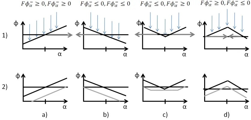
A visual representation of the derivative selection process is shown in Figure 3.6. The images in the top row represent each of the four cases described by (3.23). Imagine stand-ing at a point within Ω and lookstand-ing forward or backward along an arbitrary direction, α+ orα−, respectively. In each of the images, this point is represented by the tick mark on the αaxis. The dark slanted lines represent values of φ(α, t1) and the horizontal lines
large grey arrows designate the direction of front propagation or wind direction. The smaller arrows show how the function φ is actually evolving per (3.23) for F >0. The bottom row of images shows a dark line representing the original function,φ(α, t1) along
with a grey line representing the same function after it has evolved with time φ(α, t2).
Figure 3.6: Visual representation of the derivative selection process for the ENO scheme
If the derivatives on either side of the given point with respect to α are either both positive or both negative as in casesa andb, the derivative is calculated using an upwind stencil. If the derivatives on either side of the point differ in sign as in cases c and d, φ does not have C1 continuity at that point. In case c, two fronts are propagating away
from each other. At points of C0 continuity between these fronts, the derivative is set
The level set time step size, ∆t, is chosen according to the conditional stability re-quirement known as the Courant-Friedrichs-Lewy (CFL) condition that requires |ν| ≤1, where ν = F∆t/∆x is known as the Courant number and ∆x is the level set grid spacing.[20] This condition prevents the front from propagating further than one grid space during a single time step.
3.3.2
Isolated Pore Detection Algorithm
As the matrix grows and fronts between matrix and empty space propagate away from the fiber bundles, multiple fronts may intersect and begin growing together. At some point, these intersecting boundaries may completely surround an empty space, forming a closed pore that is isolated from the part boundary.[6] The algorithm used to detect these pores is similar to that developed by Jin, et al.[19]
The algorithm developed to detect pores upon formation and prevent the level set method from advancing the solid front inside the pore requires that the empty space, Ω+, be separated into two categories. In the following, an active boundary is defined as
by Ωc. In other words,
Ωc ⊂Ω+ (3.24)
Ωo= Ω+−Ωc (3.25)
The pore detection algorithm is executed at every time step during the evolution of the level set to determine which areas of Ω+ are in Ω
c. More precisely, the algorithm identifies which grid points in the level set grid are located within a closed region and creates a concentration variable that is used to set the propagation velocity, F, at those nodes to zero. The concentration variable, u(xij), is defined in the domain Ω+. Values
of u(xij) are zero in Ωc and unity in Ωo.
u(xij) =
�
1 ∀xij ∈Ωo
0 ∀xij ∈Ωc (3.26)
The concentration variable is then used as follows:
F =uΨ (3.27)
where Ψ will be defined in section 3.4 and is the propagation speed normal to the front dictated by reactant concentrations at the continuum level. Therefore, if a grid pointxij is in Ωc, then u(xij) = 0 and F(xij) = 0 as well and propagation stops there.
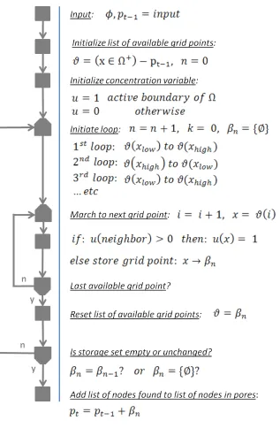
After the grid points are put in order, the algorithm follows the flowchart in Figure 3.7. The level set function, φ, and collection of grid points that were determined to lie in pores in the previous time step pt−1 are passed to the algorithm as input.
p=x∈Ωc (3.28)
The set ϑ is defined as all the grid points that could potentially be located in a pore at the beginning of a level set time step and are not in Ωc already.
ϑ =x∈Ωo = (x∈Ω+)−pt−1 (3.29)
ϑis gathered once for every time step. For earlier time steps, it is possible thatpt−1 ={∅},
so ϑ = x ∈ Ω+ in this case. The set β shown in Figure 3.7 is a version of ϑ that
is constantly changing and is reset at the beginning of every iteration. Its use allows simpler indexing and data storage, but it has the same physical significance as ϑ. Grid points that are found to lie in Ωc are added to a set p at the end of the pore isolation algorithm. The set p is never reset, so grid points are stored throughout the level set simulation.
zero, then u(ϑk) = 1, meaning that the current grid point is in Ωo if any of its neighbors are in Ωo, or in other words, gas is available at xk if it is available at a neighboring grid point.
In order to handle complex geometries, this process must be repeated. However, after u(xs) = 1 wheresis some number, the possibility thatxslies in an isolated pore has been ruled out, so it is removed fromϑ. For successive iterations, convergence is reached more quickly if the algorithm checks the points in reverse order, so the algorithm marches from ϑ(xhigh) to ϑ(xlow) in the second iteration. The algorithm continues to pass through the available grid points, reversing order in which points are checked with each pass. If the size of the set ϑ does not shrink from one iteration to the next, or if there are no grid points left in the set, the algorithm stops, and ϑ is appended to p.
2D Assumptions
section, while longitudinal fibers are represented by quasi-elliptical fiber bundle cross sections.
If the foregoing pore detection algorithm is implemented directly on a woven preform cross section, the long transverse fiber cross sections would cause isolated pores to be detected prematurely. Figure 3.8 illustrates the root of this issue and the assumptions made to overcome it. As shown by the legend at the bottom, the black sinusoidal lines represent transverse tows, the dark grey quasi-ellipses represent longitudinal tow cross sections, and the light grey areas designate areas occupied by silicon carbide matrix ma-terial. In this example, the bottom edge of each picture is considered an active boundary and is the source of MTS vapor. The curved arrows in the leftmost image show poten-tial pathways available for gas transport to the specimen interior. Note that the MTS vapor is allowed to pass around the transverse fibers. In three-dimensional space, this would be perfectly acceptable, but if the longitudinal and transverse fibers are repre-sented together by a single level set function, this pathway would be blocked and the pore detection algorithm would deem area Ωo inaccessible.
Figure 3.8: Pictorial representation of assumptions used to model pore isolation in two dimensions
by redefining Ω+ and Ω− in (3.20):
Ω−S =�Ω−T ∪Ω−L�
� �� �
solid Ω+S =�Ω+T ∩Ω+L�
� �� �
empty space
The separate domains, ΩT and ΩL, have separate level set functions that are evolved simultaneously. The pore detection algorithm is implemented to detect Ωc in ΩL only. In this way, matrix growth occurs throughout the specimen until an area is isolated by the longitudinal fibers only. To reflect this concept, (3.24) and (3.25) are rewritten
Ωc ⊂Ω+L (3.30)
Ωo= Ω+L−Ωc (3.31)
To understand the following it is important to note that although Ωo and Ωc are defined by ΩL, they correspond to regions in ΩT and ΩS because ΩT, ΩL, and ΩS overlap. Isolated pores are now defined as follows:
Ωp = Ω+S ∩Ωc (3.32)
of both ΩT and ΩL that correspond to Ωc. The rightmost image shows a representation of ΩS along with an isolated pore, Ωp that has developed.
3.3.3
Porosity and Surface Area
Values for effective porosity, �, and surface area, Sa, are required to calculate Def f and Ri as dictated by (2.7) and (3.2), respectively. Isolated pores inhibit gas diffusion during CVI, and therefore are not included in the calculation of effective porosity, �.
�= meas
�
Ω+S −Ωp�
meas(ΩS) (3.33)
and surface area is calculated similarly to � as
Sa= meas
�
Γ(Ω+S −Ωp)� meas(ΩS)
(3.34)
where Γ(Ω) refers to the sections of Γ defined by Ω or in other words, the boundary around Ω.
Since isolated pores contribute significantly to the final porosity of the part, they must be included when calculating the total specimen porosity,ε.
ε= meas
�
Ω+S� meas(ΩS)
(3.35)
cell is defined as the area enclosed by four level set grid points, this method approximates the void space in a given cell using a polygon. Linear interpolation is employed to estimate where Γ(t) crosses the boundaries of each cell. For example, the location of point F in Figure 3.9 is determined by linear interpolation based on the location of pointsA and B and their respective φ values. The location of point G is determined from points B and C, and so on. Porosity and surface area for cell ABCD are approximated by calculating the area and boundary length of polygon FBGHDE, respectively
3.3.4
Verification Solutions
Figure 3.9: Schematic of poros-ity approximation for an exem-plary single cell
To verify the level set algorithm augmented with pore isolation capability, a simple numerical experiment was conducted and the results were compared with exact calculations. A schematic of the experiment is shown in Figure 3.10. Nine circles were placed in a square do-main and arranged in a three by three lattice formation representing nine uniformly-spaced, cylindrical bundles of carbon fiber. The boundaries of each of the circles were propagated outward past the point of intersection. The pore detection algorithm was used to stop propa-gation of the circle boundaries in areas with no path to
points at which they meet is known, and the area occupied by the final shape can be precisely calculated.
Figure 3.10: Visual results of a numerical experiment using different grids
The mesoscale model is responsible for providing values of effective porosity and surface area to the continuum level model, so to test its accuracy with the numerical experiment, porosity for the whole domain was calculated. At the end of each experiment, porosity was calculated as the ratio of area not contained by the final shape to the total area within of domain.
Figure 3.11: Results from a numerical experiment using the level set and pore isolation algorithms
Error from Grid Resolution and Pore Structure Calculations
curves in the contour plots that Matlab outputs to display Γ(t) are also created using linear approximations. Figure 3.12 shows how sharp corners and high curvature are represented by Γ(t = 0) when the grid resolution is relatively low. The dotted lines show the level set grid and Γ(t = 0) is shown bold. Contours for other constant values of φ(t = 0) are also represented here using thin lines. Note that values of φ0 were initially
assigned a value of either one or zero, and that a two-dimensional interpolation scheme was later used to define Γ(t = 0) for this plot. According to the picture, this grid may be too coarse to sufficiently capture Γ(t). However, also note that the methodology described in section 3.3.3 would very nearly calculate length of Γ(t) and the area of the void space it outlines. Therefore, we will assume that if the grid resolution is high enough to sufficiently capture geometric details in a Matlab contour plot, then it is high enough for the algorithm described above to effectively calculate the porosity and surface area as well.
Figure 3.12: Interpretation of small details on a coarse grid
Error from the Pore Isolation Algorithm
Level set grid resolution, grid point placement, and time step size indirectly effect the performance of the pore isolation algorithm outlined in section 3.3.2. Figure 3.10 shows visual results of the nine circle experiment on two different grids. Careful inspection will show that the cusp between the circle boundaries looks different depending on the grid resolution. These results are represented by the first two data points on the dark solid line in Figure 3.11, in which higher positive error values mean the calculated porosity was greater than the true porosity.
line in Figure 3.11. The three results shown all use a time step corresponding to ν = 1 for the highest grid resolution (400 x 400 grid points).
The boldest of the resulting boundaries corresponds to the boldest grid lines and designates the final result with the lowest resolution (100 x 100 grid points). Note that the bold boundaries do not form a full cusp where the two circles intersect. Boundary propagation has stopped before the circle boundaries intersected each other because the pore isolation algorithm could no longer detect an opening between them. The boundaries also appear to meet because the function is linearly interpolated across the gap between them. The pore detection algorithm can only detect pathways from one grid point to its neighboring grid points, and since there are no grid points located between the two circles, no pathway was found.
Figure 3.13: Cusp region in Figure 3.10 for three different grids
these circles, infinitely small time steps would be needed, or the boundaries would need to reach this exact point at a time step for growth to stop when this point is reached.
Figure 3.14: Close up of area outlined in Figure 3.10 with boundaries for the previous time step
3.4
Multi-scale Solution Approach
The finite element formulation was implemented in Matlab to facilitate a simple interface between the continuum level finite elements and the level set mesoscale model. The data transfer between the two scales is outlined in Figure 3.15 where the two box styles differentiate the two scales.
bydt, (dt ≥∆t) and its value is left as user input. Although the finite element equations are quasi-steady, dt will be called the finite element time step because it dictates how often the finite element equations are resolved.
Propagation speed in the level set simulation is dictated by the local species concen-tration, which is calculated at the continuum level.
Ψ = RM T S,m Saρ˜SiC
λSiC λM T S
MSiC MM T S
(3.36)
The nodal reaction rate, RM T S,m, has units of mass of MTS per volume per time. The equation shown above gives Ψ units of length per time or velocity. This is assumed to be the propagation velocity normal to the surface. Recall that the propagation velocity is set to zero in isolated pores per (3.27).
porosity calculated from the level set must be passed back to the continuum level. The level set grid is defined so that every finite element node lies on top of one grid point. In this way, each finite element can be linked to a collection of grid cells. When surface area is calculated, it is integrated over all the level set cells within one finite element and stored as an elemental value. Surface area Sa is considered local value in (3.2), so elemental values are used in the right hand side of (3.11). For some analyses, it may be best to use elemental values of effective porosity, �, in (2.7a), but for the time being, global values of effective porosity (single values for the entire continuum domain) are used in this work.
The primary reason that a global value of � is used is that the elements do not encompass a large enough area to use localized values without encountering numerical issues. For instance, one element could lie completely outside of any pores, making its porosity zero, causing zeros valued diffusivities and a singular system stiffness matrix.
3.5
Processing Examples
simulation only corresponds to a latter fraction of the total CVI process time.
3.5.1
Image Segmentation and Diffusivity Approximation
A result of work done at NASA Glenn was the ability to identify fibers, matrix, and voids in CMC cross sectional images based on pixel intensity.[21] Images were separated into regions representing transverse tows, longitudinal tows, matrix material, and empty space. Specimen porosity was calculated based on the number of pixels designating regions of empty space. This type of image is useful because the segmented preform geometry can be used directly as mesoscale model input, and a clear comparison can be made between the matrix growth in the simulation and the matrix approximation provided by the image.
Such a comparison provides a qualitative estimation of the accuracy of the model parameters. In section 3.2.2, both the diffusivity and the reaction rate were estimated due to their unavailability and their dependence on a number of unknown environmental factors. However, the estimate for the reaction speed is based directly on test data, whereas the gas diffusivity is based on a number of assumptions. The Joback modification of Lydersen’s method described in section 3.2.2 is merely an estimation technique for determining the critical properties, and recall that values for neither ∆T nor ∆V could be found for the functional group > Si <, so values for > C < were used instead. This estimate was based on a knowledge of the periodic table alone, and a correlation to its physical relevance was as of yet unknown. This method was used to calculate an estimate
Figure 3.16 compares a segmented image of a 5-harness satin weave cross section with the model results using a value of DM T S,M ixture reduced from the original estimate by a factor of 30. The diffusivity, reaction rate, and other parameters used are shown in Table 3.1. The reaction rate for this model was estimated from test results.[15] For these results, mesoscale evolution was assumed to last for 15 hours and guesses were made as to the best values for grid points per element, Courant number (ν), and finite element time step (dt).
This particular preform geometry is a good test case for estimating the accuracy of the model diffusivity because the mechanics are relatively simple. In this particular cross section, the tow spacing and the ply stacking is such that no isolated pores form according to the definition in section 3.3.2, and therefore, the matrix geometry is not influenced by the implementation of the pore detection algorithm outlined in section 3.3.2.
Figure 3.16: Model output and segmented specimen cross section
Table 3.1: Initial model parameters used with a model refinement study
KM T S 8.33×10⁻⁶kg/m2s
DM T S,mix 1.56×10⁻⁴m2/s ptest 454.6P a
T 965◦C
MM T S 0.1495kg/mol MSiC 0.00467kg/mol
τ0 1
the boundaries tends to increase as the value of DM T S,M ixture is decreased relative to the reaction rate, effectively increasing the Sherwood number. The level of thickness varia-tion shown here and small difference between the calculated porosity from the segmented image (< 5%) and the simulation indicate that the diffusivity value used here is rela-tively close to the true value for this particular process. Therefore, the calibrated value of DM T S,M ixture will be used in the grid refinement and time step size studies described in the next section.
3.5.2
Refinement Study
involved in matrix growth are a bit more complicated. The longitudinal tows are oriented in such a way that isolated pores will form. While a majority of the enclosed pore space does not form until the evolution process is nearly complete, its formation engages the pore isolation algorithm described in section 3.3.2, and therefore, the porosity calculation is subject to error of the type described in section 3.3.4.
Per the discussion in section 3.3.2, the longitudinal and transverse fibers are modeled separately, so that the pore isolation algorithm can be implemented using the longitu-dinal tows only. Figure 3.17 shows model output for this specimen with ΩL and ΩT displayed separately. The grey regions represent the carbon fiber preform geometry, and the white regions show the matrix growth around this the preform. In these images, re-gions corresponding to Ωc are highlighted in green and correspond to areas where matrix growth was automatically stopped during the simulation.
element edge, and this quantity will be referred to as level set grid points per element. Temporal model refinement can also be accomplished at the continuum level by up-dating the values for porosity and surface area more frequently. Decreasing the value of dt increases the number of times that the reactant concentration distribution is re-calculated. On the mesoscale, decreasing the Courant number, ν, decreases the size of the level set time step, ∆t, and increases the number of level set time steps between each re-calculation. The effect of the values of bothdt and ν will be studied.
The effect of changing the number of level set grid points per element on porosity values and model runtime is shown in Figure 3.18. For a given analysis, the level set function, φ, needs to be generated once. Most of the time involved in generating this function is spent smoothing it, so that there are not jump discontinuities between Ω+ and
Ω−. The smoothing algorithm iterates so that φ approaches a signed distance function, and this is the largest contributor to the function generation time shown in blue. This is added to the model runtime, and the total is used to quantify the effect of refinement on computational expense. In each chart, model runtimes are shown on the left ordinate and specimen porosities are listed on the right. The calculated porosity for the highest level of refinement is displayed in black and the deviation from that value for all other cases is displayed in terms of percent differences.
decreases ∆t, so values on the leftmost end of these charts (50 grid points per element) result from using the highest level of refinement for both ∆x and ∆t. Note that the calculated porosity does not approach a single value with increasing grid refinement. Also, porosity values do not change by much (< 5%). The source of the variation in results seen here is most likely caused by the mechanisms discussed in section 3.3.4, particularly the type illustrated by Figure 3.14. Note that a smaller time step size or higher level of grid refinement does not guarantee that two approximated fronts will meet closer to their true intersection point. This means that error values may continue to fluctuate even as the grid is refined because the pore size will change depending on where the fronts intersect.
Although there is no noticeable trend in porosity values, total model runtimes are strongly influenced, and are roughly an order of magnitude larger with 50 grid points per element than they are with only 20 grid points per element. Another point of interest is that decreasing ν increases the model run time by a larger percentage for models with high grid resolution than it does for lower resolution models. In this case, reducing ν to a quarter of what it was causes a 30% increase in runtime for the model with 20 grid points per element; whereas total runtime increases by 100% for the model with the highest grid resolution. If the grid appears to effectively capture the preform geometry visually, increasing the grid resolution will not likely improve the accuracy of the results and will greatly increase computational cost.
is explored in Figure 3.19 for two level set grids. When the grid is fixed, ∆x does not change so for a given value of F, ∆t∝ν. According to Figure 3.19, the value of ν when ∆x is constant does directly effect the model output. In the results shown, the porosity varies as much as 6% when the largest recommended value ofν is used. These plots also confirm the conclusion made with Figure 3.18 that increasing the grid refinement has a very large effect on total model runtime. Perhaps less apparently, decreasing ν also decreases the variation between the results using different grid refinements. Here, with ν = 1, moving from 20 grid points per element to 40 grid points per element changes the porosity by 2.8%. On the other hand, with ν = 0.625, this refinement changes the porosity by only 1.3%. Therefore, it is in the users best interests to choose a relatively low value for ν.
Table 3.2: Model parameters used for final results
KM T S 8.33×10⁻⁶kg/m2s
DM T S,mix 1.946×10⁻⁴m2/s ptest 454.6P a
T 965◦C
MM T S 0.1495kg/mol MSiC 0.00467kg/mol
τ0 1
∆t= 0.625 as well, so at a certain point, decreasing the size of thedteffectively decreases ν.
3.5.3
Final Processing Results
Since the size of the level set time step had a significant effect on the calculated porosity of the model, the diffusivity was re-evaluated so that the calculated model porosity more closely matched the porosity calculated using image segmentation. Note the level of agreement between the results shown in Figure 3.21. The new value of DM T S,mix is shown in Table 3.2. In this case thirty grid points per element were found to represent the geometry sufficiently, and the time step refinement parameters were chosen based on the results in the previous section. Apart from the model refinement parameters, only the value of DM T S,mix was changed as a result of this re-evaluation.
Figure 3.21: Model output using new model refinement parameters and a segmented specimen cross section
whereas only the top edge is an active boundary in the bottom image. Note the difference in matrix thickness near the bottom edge of the specimen. The resulting porosity increase is roughly 70%. Therefore, changing the processing setup in this way could significantly reduce the material performance.
Figure 3.22: Model output for two processing conditions
conditions were the same in this case, and porosity values were not available. Never-theless, the simulation was run and the results are shown here so a comparison of the predicted geometry and an actual CT scan of the cross section could be made. Figure 3.23 shows the model output next to the CT scan. The color scheme of the model output was chosen to approximate that of the scanned image. Note that because a well defined preform geometry was not available, the geometry used as input is an approximation to the true geometry using ellipses and sinusoidal lines. Given the uncertainties in the processing conditions, the agreement is qualitatively good.
In Figure 3.24, the predicted mesoscale structure is overlayed with the CT scan. The black lines show the outline of the simulated carbon fiber preform approximation, and the pore space resulting from the simulation is highlighted in red. Although this figure may be a bit harder to interpret, it provides a more direct comparison between the simulation and reality.
Chapter 4
Oxidation Modeling
4.1
State of the Art
Oxidation occurs in C/SiC CMCs when high temperature oxygen gains access to the carbon fiber reinforcements. In previous work,[6] it was assumed that oxidation was governed by the following reaction:
C+O2 →CO2 (4.1)
whereO2 andCO2 were the only vapor species present during the oxidation process. For
simplicity, the same assumption will be made for this work.
Exposure to atmospheric oxygen is provided by the pores created during the manu-facturing process and the cracks that form after cool down. Oxidation in environments above 450◦C (840◦F) is the primary disadvantage to using CMCs,[1] so increasing the reliability of predictions is a crucial step in determining the overall life of a component.