Model Comparison Tests to Determine Data Information Content

Model Comparison Tests to Determine Data

Information Content

H.T. Banks

, J.E. Banks

_{, Kathryn Link}

_{, J.A. Rosenheim}

_{, Chelsea Ross}

_{, and K.A. Tillman}

_{Center for Research in Scientific Computation}

North Carolina State University

Raleigh, NC 27695-8212 USA

and

@

_{Department of Environmental Science}

Division of Sciences and Mathematics (SAM)

University of Washington, Tacoma

Tacoma, Washington 98402

and

+

_{Department of Entomology and Nematology, and Center for Population Biology}

University of California, Davis

Davis, CA 95616

October 31, 2014

Abstract

In the context of inverse or parameter estimation problems we demonstrate the use of statistically based model comparison tests in several examples of practical interest. In these examples we are interested in questions related to information content of a particular given data set and whether the data will support a more complicated model to describe it. In the first example we compare fits for several different models to describe simple decay in a size histogram for aggregates in amyloid fibril formation. In a second example we investigate whether the information content in data sets for the pestLygus hesperusin cotton fields as it is currently collected is sufficient to support a model in which one distinguishes between nymphs and adults. Finally in a third example with data for patients having undergone an organ transplant, we question whether the data content is sufficient to estimate more than 4 of the fundamental parameters in a particular dynamic model.

Key Words: Ordinary least squares, model comparison in inverse problems, information content

1

Introduction

Uncertainty quantification in the context of estimation of parameters has become a focus of increased at-tention in recent years. As mathematical models become more complex with multiple states and many parameters to be estimated using experimental data, there is a need for critical analytical tools in model val-idation related to the reliability of parameter estimates obtained in model fitting. Methodology is desirable to distinguish between lack of identifiability in a model (often formulated in a generalized algebraic context) versus local insensitivity with respect to changes in particular parameters versus lack of information content in a given data set. A recent concrete example involves previous HIV models [1, 4] with 15 or more param-eters to be estimated. In [2], using recently developed parameter selectivity tools [3] based on parameter sensitivity based scores, the authors showed that many of the parameters could not be estimated with any degree of reliability. Moreover, it was found that quantifiable uncertainty varies among patients depending upon the number of treatment interruptions (perturbations of therapy). This leads to afundamental question

of how much information with respect to model validation can be expected in a given data set or collection of data sets. In this note, we consider one tool that may be used in attempts to answer this question.

Here we demonstrate the use ofstatistically based model comparison testsin several examples of practical interest. In these examples we are interested in questions related to information content of a particular given data set and whether the data will support a more detailed or sophisticated model to describe it. In the first example we compare fits for several different models to describe simple decay in a size histogram for aggregates in amyloid fibril formation. In a second example we investigate whether the information content in data sets for the pest Lygus hesperus in cotton fields as it is currently collected is sufficient to support a model in which one distinguishes between nymphs and adults. Finally in a third example with data for patients having undergone an organ transplant we question whether the data content is sufficient to estimate more than 4 of the fundamental parameters in a specific dynamic model. In the next section we recall the fundamental tests to be employed here.

2

Summary of ANOVA Type Statistical Comparison Tests

In general, assume we have an inverse problem for the model observationsf(t, q) and are givennobservations. We define

Jn(q) =Jn(Y, q) =

1

n n

∑

j=1

[Yj−f(tj, q)]2 (1)

where our statistical model has the form

Yj=f(tj, q0) +Ej, j= 1, . . . , n.

Here,q0is the “true” value ofqwhich we assume to exist. We useQto represent the set of all the admissible

parametersq.

We make the standard statistical assumptions [5, 7, 9]:

• A1) The random variables {Ej}∞j=1 are independent and identically distributed with E(Ej) = 0 and V ar(Ej) =σ2.

• A2) Qis a compact subset of Euclidian space ofRp _{andf(t, q) is continuous on [0, T]× Q.} • A3) Observations are at {tj}nj=1 in [0, T]. For some finite measureµon [0, T],

1

n n

∑

j=1

h(tj)−→

∫ T

0

h(t)dµ(t)

as n→ ∞, for all continuous functionsh.

• A4) J0(q) =

∫T

0 (f(t, q0)−f(t, q))

2_{dµ(t) =σ}2 _{has a unique minimizer inQatq} 0.

Letqn =q_OLSn (Y) be the OLS estimator forJn with corresponding estimate

ˆ

for a realizationy={yj}. That is,

qn(Y) = arg min

q∈QJn(Y, q)

and

ˆ

qn = arg min

q∈QJn(y, q).

One can then establish a series of useful results (see [5, 7] for detailed proofs).

Theorem 2.1. Under A1) to A4), qn_=qn

OLS(Y)−→q0 asn→ ∞ with probability 1.

Remarks:

• In most calculations, one actually uses an approximation fN _{to f (often the numerical solution to}

ODE or PDE for modeling a dynamical system). In this case one tacitly assumesfN _{will converge to} f as approximation improves.

• There are also questions related to the approximations of setQwhen it is infinite dimensional (e.g., in case of function space parameters such as time dependent or probability distribution parameters) by finite dimensional discretizationsQM _{(see Chapter 5 of [7]).}

• For extensive discussions related to these questions, see [8] as well as [5] where certain related assump-tions A5), A6) on convergencesfN _{→f andQ}M _{→ Q are given.}

• We will ignore these issues here since they are only tangentially related to our examples, keeping in mind these approximations will also be of importance in many practical uses of the methodology discussed below.

We will need further assumptions to precede (these will be denoted by A7)–A11) to facilitate reference to [5, 7]). These include:

• A7) Qis finite dimensional inRp andq0∈ Q.

• A8) f :Q →C[0, T] is aC2 _function.

• A10)J = ∂2J0

∂q2 (q0) is positive definite.

• A11)QH={q∈ Q|Hq=c} whereH is anr×pmatrix of full rank, andcis a known constant.

In many instances, including the motivating examples discussed here, one is interested in using data to question whether the “true” parameterq0can be found in a subsetQH ⊂ Qwhich we assume for discussions

here is defined by the constraints of assumption A11). Thus, we want to test thenull hypothesisH0: q0∈ QH.

Define then

qn_H(Y) = arg min

q∈QH

Jn(Y, q)

and

ˆ

q_Hn = arg min

q∈QH

Jn(y, q).

and observe that Jn(Y,qˆHn) ≥ Jn(Y,qˆn). We define the related non-negative test statistics and their

realizations, respectively, by

Tn(Y) =n(Jn(Y, qHn)−Jn(Y, qn))

and

ˆ

Tn =Tn(y) =n(Jn(y,qˆnH)−Jn(y,qˆn)).

One can establish asymptotic convergence results for the test statisticsTn(Y)–see [5]. These results can,

in turn, be used to establish a fundamental result about much more useful statistics for model comparison. We define these statistics by

Un(Y) =

Tn(Y) Jn(Y, qn)

, (2)

with corresponding realizations

ˆ

un=Un(y).

Theorem 2.2. Under the assumptions A1)–A4) and A7)–A11) above and assuming the null hypothesisH0

is true, thenU_n converges in distribution (asn→ ∞) to a random variable U(r)

Un−→D U(r)

having a chi-square distributionχ2_{(r)with rdegrees of freedom.}

We note that if one is dealing with vector observations withn=n1+n2 total component observations

as we do in two of the examples below, then asymptotic theory requires thatn1→ ∞andn2→ ∞.

An example of theχ2_{density is depicted in the figure below where the density forχ}2_{(4) (χ}2_{withr= 4}

degrees of freedom) is graphed. In this figure two parameters (τ, α) of interest are shown. For a given value

τ

p(u)

α

Figure 1: Example ofU ∼χ2_{(4) density}

τ, the value α is simply the probability that the random variable U will take on a value greater than α. That is,P rob{U > τ}=αwhere in hypothesis testing,αis the significance level andτ is the threshold.

We wish to use this distribution to test the null hypothesis, H0, for Un ∼χ2(r). If the test statistic,

ˆ

un> τ, then wereject H0 as falsewith confidence level (1−α)100%. Otherwise, we do not reject H0. For

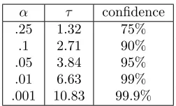
our examples below, we use aχ2_{(1) table, which can be found in any elementary statistics text or online.}

Table 1: χ2₍₁₎

α τ confidence .25 1.32 75%

.1 2.71 90% .05 3.84 95% .01 6.63 99% .001 10.83 99.9%

To test the null hypothesis H0, we choose a significance level α and useχ2 tables to obtain the

corre-sponding thresholdτ =τ(α) so that P(χ2_{(r)> τ) =α. We next compute ˆu}

n=τ and compare it to τ. If

ˆ

un> τ, then we rejectH0as false; otherwise, we do not reject the null hypothesisH0.

2.1

Weighted Least Squares

The model comparison results outlined can be extended to deal with weighted least squares problems in which measurement errors are independent with E(Ek) = 0 and V ar(Ek) =σ2w2(tk), k = 1,2, . . . , n, where w is

some known real-valued function withw(t)̸= 0 for anyt. This is achieved through rescaling the observations in accordance with their variance (as discussed in [7]) so that the resulting (transformed) observations are identically distributed as well as independent.

3

Size distribution of aggregates in amyloid fibril formation

3.1

Size distribution of aggregates in amyloid fibril formation

0 1000 2000 3000 4000 5000 6000 0

20 40 60 80 100

Fibril Size (monomers)

Number of Polymers Per Bin

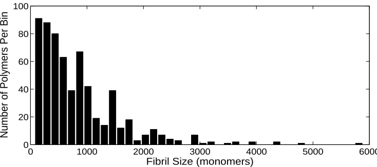
Figure 2: Experimental distribution of the samplexi, 1≤i≤n,representing the measured sizes of polymers

(the number of polymers below a certain size (145 monomers) is unknown). The total size of the sample is

n= 626.

3.2

The Exponential, Weibull and Gamma Distributions

On initial observation, the data appears to be well suited to an exponential distribution. The exponential distribution probability density function is defined asE(x;λ) =λe−λx_{. Below in Figure 3 the exponential}

function with varying values of λis depicted. Note that when fitting the data, an additional parameter A

was added to the exponential function resulting in a total of two parameters and the function to be defined for these purposes as

E(x;A, λ) =Aλe−λx.

The Weibull distribution probability density function is defined as (for the purposes of modeling the data we again add the additional parameterA)

W(x;A, λ, k) =Akλ(λx)k−1e−(λx)k, x≥0.

Note that if we takek= 1 we have thatW(x;A, λ,1) =E(x;A, λ).

This function is shown plotted below with several values ofk. We can see that whenk= 2 ork= 1 the function also bears a resemblance to the shape of our data.

The probability density function of the gamma distribution is defined as (we again include the additional parameterA for modeling purposes)

G(x;A, k, λ) =A λ k

Γ(k)x

k−1_e−λx _{forx >0 andk, λ >0,}

where Γ(k) is the gamma function evaluated atk. We can see in the figure below that when k = 1 and

λ= 0.5, the gamma probability density function again has a similar shape to the data. Since we know that Γ(1) = 1, we can see that when we takek= 1 we have thatG(x;A,1, λ) =E(x;A, λ).

Thus an interesting question is whether we can obtain an statistically better fit to the data in Figure 2 by allowing an additional free parameterkin either the Weibull or gamma distribution in comparison to the two parameter (A, λ) exponential model.

3.3

Results using the comparison tests

We tested the following hypothesis and alternative for two different alternative models: a Weibull and a gamma distribution:

0 0.5 1 1.5 2 2.5 3 3.5 4 4.5 5 0 0.2 0.4 0.6 0.8 1 1.2 1.4 1.6 1.8 2 x E(x; λ )

λ = 0.5

λ = 1

λ = 1.5

(a) Exponential probability density function

0 0.5 1 1.5 2 2.5

0 0.2 0.4 0.6 0.8 1 1.2 1.4 1.6 1.8 2 x W(x; A, λ , k)

λ = 1, k=2

λ = 1,k=1

λ = 1, k=2/3

λ = 1,k=1/5

(b) Weibull probability density function

0 2 4 6 8 10 12 14 16 18 20 0 0.05 0.1 0.15 0.2 0.25 0.3 0.35 0.4 0.45 0.5 x

G(x; A, k,

λ

)

k=1, λ = 0.5 k=2, λ = 0.5 k=3, λ = 0.5 k=5, λ = 1 k=9, λ = 2

(c) Gamma probability density function

Figure 3: Graphical comparisons of the exponential with different values of λand the Weibull and gamma with different values ofλandk.

• HA: The alternative model with an unrestricted additional parameterkprovides a significantly better fit than the exponential model (corresponding to the restrictionk= 1).

When comparing the best fits of the exponential vs. the Weibull distributions we obtained the following results: Jw

n = 1.4359×10−4,Jne= 1.6081×10−4, ˆTnew = 4.6495×10−4, and ˆuewn = ¯τ = 3.2381. In this case

we cannot reject the null hypothesis at the 95% or higher level. We can reject at the 90% confidence level. When comparing the best fits of the exponential vs. the gamma distribution we obtained the following results: Jg

n= 1.4277×10−4,Jne= 1.6081×10−4, ˆTneg = 4.8693×10−4, and ˆuegn = ¯τ= 3.4105. Again in this

case we cannot reject the null hypothesis at the 95% or higher level but we can reject at the 90% confidence level.

4

Lygus hesperus

Population Dynamics: Model Comparison and

Parameter Estimation

Lygus hesperus is a prevalent insect in California which feeds on cotton and other plants [11]. Given a

techniques to determine which model is more appropriate, given the population dynamics and the nature of the data.

4.1

Data

Our main database consists of over 1500 data sets (comprising over 500 distinct fields) ofL. hesperuscounts. One data set is characterized by the following: a designated pesticide control advisor (PCA) counts the number of L. hesperusfound in a sample of field sweeps (50 large net sweeps = 1 sample) at intermittent times from early June to early August. Some PCAs distinguish between nymph and adult specimens whereas others simply count total insects caught; therefore only some data sets consist of nymph and adult counts for each time point. In addition, the fields can vary by the absence or application (and variety) of pesticide treatments. We assume that field counts are independent between years (i.e. if one field is sampled in 2004 and 2005, we consider these data sets to be independent).

To narrow down this vast collection of data, and to start with the simplest case, we choose a sub-collection of the data consisting only of data sets corresponding to fields that were untreated by pesticides for a minimum of 2 uninterrupted months, in which PCAs counted both nymphs AND adults. There were at least 40 data sets of this nature. By starting with this sub-collection, we are able to study the insect population dynamics which are not directly affected by pesticides. We note that pesticide usage on nearby crops can have an indirect effect on these crops, but choose to ignore this potential effect for now, as it is largely unknown and variable. In addition, this allows us to propose a 2-dimensional population model. These pesticide free counts occurred between the months of June and August. In this model, we choose 6 of these data sets as a preliminary study. An example of one data set can be seen in Table 4. Note that there are several data points where adult and nymph counts are non-integer values. This is due to the fact that several fields were so large that PCAs chose to do a number of samples within one field on one particular observation day and averaged the results.

4.2

Model

We assume there are 2 distinct population classes: nymphs and adults. We will denote their populations as x1(t) and x2(t) respectively, where t is time measured in months (t ≥ 0). Given this particular insect

and data collection scheme, we consider t = 0 to mean June 1 (as no observations in our data sets are made before this date). For now, we will ignore the effect of pesticides on the population, and consider the population dynamics ofL. hesperusin an untreated environment. We do not assume a closed population (i.e.

dX

dt ≡

dx1

dt +

dx2

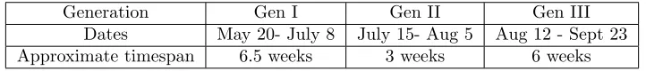
dt ̸= 0.) In addition, it is assumed that there are at least 3 generations per year. One source

[11] stated that the generation times (of the nymphs) varied depending on the time of year. They reported 3 generations ofL. hesperusnymphs in summer 1998, which can be seen in Table 2. This information may be useful when analyzing parameter estimates.

Generation Gen I Gen II Gen III

Dates May 20- July 8 July 15- Aug 5 Aug 12 - Sept 23 Approximate timespan 6.5 weeks 3 weeks 6 weeks

Table 2: Example of nymphal development time

We first consider a simple 2-dimensional ordinary differential equation model. Model A is as follows:

dx1(t)

dt =βx2(t)−γx1(t) dx2(t)

dt =γx1(t)−µ2x2(t),

(3)

whereβ is the birth rate of nymphs,γ is the transition rate of nymphs into adulthood, andµ2 is the adult

However, Model B assumes a non-trivial nymph mortality:

dx1(t)

dt =βx2(t)−(γ+µ1)x1(t) dx2(t)

dt =γx1(t)−µ2x2(t),

(4)

whereµi is the death rate forxi,i= 1,2. For both model A and B, initial conditions

X1= (x1(t1), x2(t1)) := (x1,1, x2,1)

are unknown. Note thatt1, the time of the first observation, varies between data sets. Our goal is to estimate

parameters in Model B, ˜q = {β, γ, µ1, µ2, x1,1, x2,1} using our chosen data sets (note that the parameters

in Model A are equivalent to those in Model B, with the constraint thatµ1 = 0). We will use MATLAB’s

constrained optimization tool,fminconand both ordinary least squares (OLS) and weighted least squares (WLS) techniques.

4.3

Comparison Data

In addition to our main database, we have a supplementary set of data consisting of 9 fields in which nymphs and adults counts were recorded by PCAs and subsequently counted again by our team within 7 days of the original count. Although these 9 fields are not the same as those found in the large database, they are characteristically similar, and thus can be used to make an inference on data collection error when performed by PCAs. As previously mentioned, some PCAs do not bother to count nymphs or distinguish between age classes. This is largely because the nymphs are smaller and thus harder to see amidst net debris and because the nymphs tend to cling more tightly to the plants during sweeps. Our team aimed to provide a more accurate count by (a) stirring plants more vigorously to detach nymphs before sweeping with nets and (b) more carefully removing debris from nets to allow for more thorough counts. We sought to find some ratio of the counts to compare the data from the PCAs and our team. All information is summarized in Table 3. Note that (x, y) in the column entitled “(2nd_{,PCA) Nymphs” signifies thatx= number of nymphs counted by}

our team, andy= number of nymphs counted by a PCA. Similarly, (x, y) in the column entitled “(2nd,PCA) Adults” signifies that x= number of adults counted by our team, andy= number of adults counted by a PCA. When possible (i.e. when neitherxnory was zero), we calculated a ratio for each ordered pair, which can be found in Table 3 as well.

There is a great deal of variability in the data. However we see some common trends. In 6 out of 9 fields, PCAs reported 0 nymphs, and in 1/9 fields, PCAs reported 0 adults. Our team never reported 0 adults. In all fields, the 2nd_{nymph count is greater than or equal to the PCA count. In 7/9 fields, the 2}nd_{adult count}

is greater than or equal to the PCA count.

It appears that it will be impossible to derive a quantitative measure of PCA data collection error for two reasons: 1) there is no clear pattern of PCA error for either the nymph or adult counts (although it is fairly consistent that the PCAs counted fewer insects than our team), and 2) with an exception of at most 2 fields, none of the fields used in the comparison data are included in our original set of data. In reality, this comparison set of data is comprised of one sample by PCAs and one sample by our team 7 days later, of 9 fields with no clear pattern and little to no additional information about those fields. However, the clear information we did derive from this data is as follows: we are fairly certain that the PCAs undercount the nymphs. In the 9 fields that both the PCAs and our team sampled, 6/9 fields were recorded with 0 nymph counts by the PCAs, whereas our team only recorded one field with a 0 nymph count.

This leads us to believe that using weighted least squares in our parameter estimation is important. To estimate parameters, one must search within an admissible parameter space, ˜Q, for the model parameters that produce a model output most similar to the data. In other words, one must minimize the cost functional,

Jn defined to be

Jn =Jn(y, q) =

1 2n

n

∑

i=1

k

∑

j=1

ωj(yij−mij)2, (5)

where yij = is the data point from thejth class at the ithtime point, and mij = is the model output for

the jth _{class at the i}th _{time point, given a parameter estimate. Between fields, n (the number of vector}

j= 1 corresponds to the nymph class andj = 2 corresponds to the adult class so that the total number of data points is 2n. Let Ω ={ω1, ω2}. There are formal ways of choosing Ω, but we will start with some basic

choices. If we choose Ω = {0,1}, we are ignoring the nymph counts in the search for the best parameter estimates for the model. If we choose Ω ={0.5,1}, we are giving less weight to the nymph class than to the adult class. Note that if we choose Ω ={1,1}, we return to an OLS method.

Site (2nd_{,PCA) nymphs (2}nd_{,PCA) Adults 2}nd_{:PCA nymph ratio 2}nd_{:PCA adult ratio}

1 (0.1, 0) (3.15, 2.25) n/a 1.4

2 (0, 0) (1.15, 0.5) n/a 2.3

3 (0.3, 0) (2.35, 0) n/a n/a

4 (0.15, 0) (0.9, 0.25) n/a 3.6

5 (1.75, 0) (1.85, 0.25) n/a 7.4

6 (2.1, 0) (3.5, 3) n/a 1.2

7 (4.3, 1.5) (7.05, 7.75) 2.9 0.9

8 (3.6, 0.5) (7.7, 5.33) 7.2 1.4

9 (1.15, 0.13) (3.75, 5.17) 8.8 0.72

Table 3: A comparison of 9 fields studied by PCAs and our team

4.4

Parameter Estimates and Model Comparison Test

As mentioned previously, there are differing opinions among PCAs and researchers about whether both nymphs and adults need to be counted. The reasons for these differences are varying beliefs regarding the effect of pesticides and other factors on the L. hesperus populations. We seek a quantitative measure to determine whether counting both nymphs and adults (in the manner in which it is presently done) is necessary, or if it is sufficient to simply count the total number of insects. We see that the sole difference between Models A and B ((3) and (4), respectively) is the assumption of no nymph mortality in Model A. Note that model A can be more simply written as

dX

dt =αx2(t), (6)

whereX(t)=the total number ofL. hesperusat timet(X=x1+x2), andα=β−µ2. This simpler model is

exponential in nature. One may wonder how this model could possibly be exponential in nature, when there are 2 state variables,Xandx2in one differential equation. We found consistently among PCA-collected data

that the nymph counts were almost always zero. Therefore, given the current collection strategies,X ≈x2,

and (6) truly becomes an exponential growth model. A natural question is the following: by allowing nymph mortality to be non-zero, does our model better fit the data? To address this question, using a residual sum of squares statistical test [9], we can test the null hypothesis: is the true set of parameter values, q0, in a

constrained subsetQH ofQ, which requires thatµ1= 0, or do we obtain a statistically significant better fit

allowingµ1̸= 0?

We define r equal the number of constraints applied to Q_H, and pequal the number of parameters to be estimated. According to our null hypothesis, we are only interested in constrainingµ1, and thusr= 1.

Note that it is unlikely that 6 parameters can be estimated accurately given only 30-50 total data points per data set, and the likelihood of finding local, but not global minima, decreases as we fix certain parameters. Therefore, for each data set, we estimatedqwith a variety of weights, Ω, and from those estimates, fixed the initial conditionsx1,1, andx2,1at values that most accurately reflected the data. With these two parameters

fixed, we could perform the model comparison test withp= 4. In other words, our new parameter vector to be estimated is

q={β, γ, µ1, µ2} ∈ Q.

Our fundamental question now becomes: Do we obtain an improved fit to the data for q ∈ Q vs. that obtained by restricting q∈ QH ⊂ Q, and if so, is this improved fit statistically significant?

In general, we defineQH:={q∈ Q|Hq=c}, where H is anr×pmatrix of full rank, andc is a known

Although the only true constraint is that each of these values must be non-negative, we impose the further constraint that each be less than 100. We chose 100 because we found it unlikely that any true parameter value would fall above this upper bound, and it greatly speeds up the parameter estimation process by refining the search space. Therefore,

Q= [0,100]×[0,100]×[0,100]×[0,100].

In this case, we letH = [0,0,1,0] (which is of full rank), andc= 0. This is equivalent to the constraint that

µ1= 0, which simply means that there is no nymph mortality. ThusQH is simply QH= [0,100]×[0,100]× {0} ×[0,100].

Therefore, by testing the null hypothesis H0 : q0 ∈ QH, we can determine with a definitive amount of

confidence whether we can assume no nymph mortality and thus use a simple model such as Model A to describe the data.

Time Adult Count Nymph Count

0.47 2.08 0.08

0.6 0.92 0

0.7 0.33 0

0.83 1.17 0

0.93 0.33 0

1.07 1.08 0

1.17 0.42 0

1.3 0.33 0

1.4 0.58 0

1.53 1.08 0

1.63 1.75 0.33

1.77 1.25 0.08

1.87 0.92 0

2 1.67 0

2.1 2.58 0.83

2.23 2.22 0

2.33 3.67 0

2.47 1.56 0

Table 4: Data set 1 with time (time unit is one month, June 1=0), adult count per sample (50 sweeps), and nymph count per sample. Here 2n= 18 + 18 = 36.

4.5

Results

We chose to perform this analysis on 6 data sets, with 4 choices of Ω:

Ω1={1,1},Ω2={0.5,1},Ω3={0.2,1}, and Ω4={0,1}.

As seen in Table 5, for all cases (except for data set 4 with Ω3), the confidence to rejectH0is less than 19%.

There are also three cases in which our analysis returned a negative value for U: data set 1 with Ω2 and

data set 4 with Ω2 and Ω3. However, since these values are all on the order of 10−4, we believe this is due

to numerical error. In addition, we see that many estimates for µ1 returned values relatively small and/or

close to zero. This is further evidence that it may be acceptable to assume no nymph mortality. There are cases (especially with weight Ω4 in various data sets and in data set 6, specifically, across various weights)

where our confidence level was very small, but the estimate for µ1 was not close to zero. This may be due

to several local minima within the parameter space.

Lastly we explored the effect of one’s choice of Ω on the estimates of initial conditions, x1,1 and x2,1.

As we experimented with various choices of Ω, we found that as ω1→0, the values forx1,1 andx2,1 move

toward the first data points in the given set. More specifically, once we choose ω1 = 10−3, the parameter

estimates are very close to the initial data points. However, we find it disadvantageous to consider weights close to Ω4. Even if the nymph data has a large degree of error, it is unreasonable to expect an optimization

routine to find nymph population parameters such asγ andµ1with a complete absence of nymph data. In

addition, we found that the weights that returned the best estimates of initial conditions among all data sets were Ω1 and Ω2.

0 0.5 1 1.5 2 2.5

0 0.1 0.2 0.3 0.4 0.5 0.6 0.7 0.8 0.9

Nymph Model Output vs. Data

time (months); June 1= 0

Nymph count

Data Model Output

(a) Model fit versus DS 1 - Nymphs

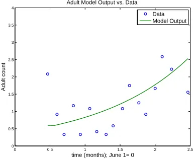
0 0.5 1 1.5 2 2.5

0 0.5 1 1.5 2 2.5 3 3.5 4

Adult Model Output vs. Data

time (months); June 1= 0

Adult count

Data Model Output

(b) Model fit versus DS 1 - Adults

Figure 4: Model fit vs. DS1

4.6

Conclusions

Data set 1 with estimated initial conditions{x1,1, x2,1}={0,0.06}

Ω Confidence qˆn _qˆn

H uˆn Jn(y,qˆn) Jn(y,qˆnH) {1,1} 3.57% {8.14, 99.74, 0.00, 7.32} {7.59, 92.97, 0, 6.77} 0.002 0.2410 0.2410 {0.5,1} 0% {9.47, 94.14, 0.00, 8.62} {8.97, 89.35, 0, 8.13} -0.0008 0.2309 0.2309 {0.2,1} 2.98% {12.79, 88.69, 0.00, 11.88} {12.02, 83.84, 0, 11.12} 0.0014 0.2241 0.2241 {0,1} 4.51% {29.36, 51.14, 6.29, 24.79} {25.47, 56.20, 0, 24.13} 0.0032 0.2145 0.2415 Data set 2 with estimated initial conditions{x1,1, x2,1}={0.01,0.22}

Ω Confidence qˆn _qˆn

H uˆn Jn(y,qˆn) Jn(y,qˆnH) {1,1} 3.91% {10.36, 88.71, 6.05, 8.60} {10.88, 96.94, 0, 9.76} 0.0024 0.0302 0.0302 {0.5,1} 3.19% {10.50, 79.42, 15.26, 7.71} {10.42, 96.06, 0, 9.30} 0.0016 0.0256 0.0256 {0.2,1} 2.52% {10.01, 84.54, 7.08, 8.13} {10.32, 94.54, 0, 9.21} 0.001 0.0228 0.0228 {0,1} 2.26% {10.08, 81.54, 8.53, 8.02} {9.98, 88.65, 0, 8.86} 0.0008 0.0210 0.0210 Data set 3 with estimated initial conditions{x1,1, x2,1}={0.03,0.05}

Ω Confidence qˆn _qˆn

H uˆn Jn(y,qˆn) Jn(y,qˆnH) {1,1} 15.77% {33.13, 50.77, 4.47, 28.17,} {32.53, 52.63, 0, 30.15} 0.0396 0.1556 0.1557 {0.5,1} 9.42% {33.83, 50.11, 4.91, 28.51} {34.12, 61.67, 0, 31.85} 0.014 0.0895 3.0895 {0.2,1} 10.06% {32.91, 50.66, 3.49, 28.49} {34.69, 59.04, 0, 32.36} 0.016 0.0498 0.0498 {0,1} 18.17% {46.60, 45.64, 32.32, 25.29} {31.78, 50.79, 0 29.39} 0.0528 0.0233 0.0234 Data set 4 with estimated initial conditions{x1,1, x2,1}={0.004,0.05}

Ω Confidence qˆn qˆ_Hn uˆn Jn(y,qˆn) Jn(y,qˆnH) {1,1} 1.13% {64.35, 66.83, 0.00, 59.63} {65.42, 67.94, 0, 60.70} 0.0002 0.5660 0.5660 {0.5,1} 3.74% {59.73, 60.96, 1.08, 54.04} {56.25, 58.26, 0 51.56} 0.0022 0.3931 0.3931 {0.2,1} 73.67% {72.15, 2.40, 77.02, 0.00} {41.47, 44.58, 0 36.92} 1.2514 2.778 2.887

{0,1} 0.8% {2.11, 99.34, 0.00, 0.00} {2.11, 99.33, 0, 0.00} 0.0001 0.1972 0.1972 Data set 5 with estimated initial conditions{x1,1, x2,1}={0.06,0.15}

Ω Confidence qˆn qˆ_Hn uˆn Jn(y,qˆn) Jn(y,qˆnH) {1,1} 5.29% {29.53, 60.42, 5.31, 25.11} {27.57, 62.05, 0, 25.50} 0.0044 0.1879 0.1880 {.5,1} 4.37% {28.55, 64.61, 0.012, 26.48} {28.11, 62.34, 0, 26.03} 0.003 0.1600 0.1600 {.2,1} 5.04% {26.85, 60.05, 1.88, 24.01} {26.41, 61.47, 0, 24.37} 0.004 0.1431 0.1431 {0,1} 1.95% {13.32, 66.62, 4.11, 11.00} {11.73, 59.00, 0, 10.15} 0.0006 0.1313 0.1313 Data set 6 with estimated initial conditions{x1,1, x2,1}={0.05,0.22}

Ω Confidence qˆn _qˆn

H uˆn Jn(y,qˆn) Jn(y,qˆnH) {1,1} 6.95% {20.61, 73.97, 19.15, 15.55} {19.93, 86.37, 0, 19.07} 0.0076 0.0856 0.0856 {0.5,1} 0% {21.45, 64.62, 27.39, 14.25} {17.82, 77.56, 0, 16.97} -0.001 0.0632 0.0632 {0.2,1} 0% {5.78, 19.80, 1.30, 4.54} {5.48, 20.06, 0, 4.59} -0.001 0.0497 0.0497 {0,1} 5.41% {10.47, 17.60, 0.81, 8.78} {13.09, 23.72, 0, 11.86} 0.0046 0.0403 0.0403

5

Model comparison in organ transplant modeling

5.1

Mathematical model description and data

We focus on modeling of the BK virus, a common pathogen (and major threat) found in kidney transplant patients-see [6] and the references therein. We describe the dynamics of the viral load V, susceptible HS

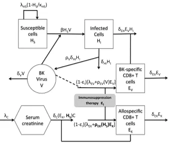
and infectedHI host cells, BKV-specificEV and allospecificEK effector CD8+ T cells and serum creatinine C with a brief description of the underlying biological model for which we base our mathematical model. Table 6 lists the state variables and Figure 5 diagrams the intracellular dynamics embodied in the model.

State Description Units

HS concentration of susceptible host cells cells/mL HI concentration of infected host cells cells/mL

V concentration of free BKV copies/mL

EV concentration of BKV-specific CD8+ T cells cells/mL EK concentration of allospecific CD8+ T cells that target kidney cells/mL C concentration of serum creatinine mg/dL

Table 6: Description of state variables

Figure 5: BKV model

Active BKV infection targets both renal tubular epithelial cells and urothelial cells. For this model, how-ever, we focus on one BKV target, the renal tubular epithelial cells. Susceptible host cells, the uninfected kidney tubular epithelial cells,HS, in the absence of infection, are assumed to proliferate through the term λHS

(

1− HS

κHS

)

HS, indicating that new epithelial cells are derived from proliferation of existingHS.

Prolif-eration is modeled by logistic dynamics withλHS being the maximum proliferation rate andκHS is the cell

cell-to-cell transmission, is represented by the term βHSV. Here we assume that one copy of virion infects

one cell. Infected host cells or BKV replicating cells,HI, lyse due to the cytopathic effect of BK virus,

repre-sented by the termδHIHIand produceρV virions before death. In addition, infected host cells are eliminated

by the BK-specific effector CD8+ T cells with rate termδEHEVHI. Free virus is naturally cleared at the rate δV by the body and a loss of viral concentration is experienced through the infection of susceptible host cells.

The cellular immune response is the key defense against the BK-viral infection. The termsλEV andδEV

represent the source and death rates of BK-specific effector CD8+ T cells. The concentration of BK-specific CD8+ T cells increases in response to the presence of free virus through the termρEVEV, whereρEV is a

bounded positive increasing function of free virus concentration. Specifically,ρEV(V) = ( ¯ρEVV)/(V +κV)

is a saturating nonlinearity with positive constants ¯ρEV and κV. The alloreactive immune response to

the transplanted kidney is incorporated into the model via a state variable, EK, which denotes the

ef-fector CD8+ T cells that specifically target the transplant. The source rate for EK, λEK, is dependent

upon the HLA donor/recipient matching conducted prior to transplantation. Similar to the BK-specific CD8+ T cells, the concentration of allospecific CD8+ T cells increases in response to the presence of susceptible host cells HS, since BK-virus targets kidney cells, represented by the term ρEKEK, where ρEK(HS) = ( ¯ρEKHS)/(HS+κKH) with positive constants ¯ρEV andκKH. The death rate ofEK is

repre-sented byδEK.

Finally, we discuss the role of creatinine in the model. Creatinine is a waste product in the blood resulting from muscle activity and is removed by the healthy kidney. Therefore, serum creatinine concentration C

is used as a surrogate for glomerular filtration rate (GFR), a commonly used index of kidney function [6]. The production rate ofCis represented byλC and when the kidney is impaired, creatinine is not effectively

filtered and its concentration increases. (Recall that the renal allograft is a site of replication. Hence, the concentration of susceptible cells reflects the health of the kidney.) To account for the negative effect of the alloreactive immune responseEK on the kidney and the positive effect of susceptible cellsHS, the clearance

rateδC is defined as follows

δC(EK, HS) =

δC0κEK

EK+κEK ·

HS

HS+κCH

.

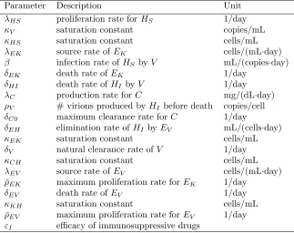
Table 7 lists the parameters used in the model.

Parameter Description Unit

λHS proliferation rate forHS 1/day

κV saturation constant copies/mL

κHS saturation constant cells/mL

λEK source rate ofEK cells/(mL·day) β infection rate ofHS byV mL/(copies·day)

δEK death rate of EK 1/day

δHI death rate of HI byV 1/day λC production rate forC mg/(dL·day) ρV # virions produced byHI before death copies/cell δC0 maximum clearance rate for C 1/day

δEH elimination rate ofHI byEV mL/(cells·day)

κEK saturation constant cells/mL

δV natural clearance rate ofV 1/day

κCH saturation constant cells/mL

λEV source rate ofEV cells/(mL·day)

¯

ρEK maximum proliferation rate forEK 1/day

δEV death rate of EV 1/day

κKH saturation constant cells/mL

¯

ρEV maximum proliferation rate forEV 1/day εI efficacy of immunosuppressive drugs

Based on the above discussion, the model is given as follows:

˙

HS =λHS

(

1− HS

κHS

)

HS−βHSV, (7)

˙

HI =βHSV −δHIHI−δEHEVHI, (8)

˙

V =ρVδHIHI−δVV −βHSV, (9)

˙

EV = (1−ϵI)[λEV +ρEV(V)EV]−δEVEV, (10)

˙

EK = (1−ϵI)[λEK+ρEK(HS)EK]−δEKEK, (11)

˙

C=λC−δC(EK, HS)C, (12)

with initial conditions

(HS(0), HI(0), V(0), EV(0), EK(0), C(0)) = (HS0, HI0, V0, EV0, EK0, C0). (13)

We note that (7)-(10) describe the immune response to the viral infection coupled with (11) and (12) describing the immune response to the transplanted kidney. HereϵI represents the efficacy of

immunosup-pressive drugs and is assumed to be scaled to less than or equal to 1. This variable serves as the controller of the system to achieve balance between under-suppression and over-suppression of the patient’s immune system.

In order to compare the effectiveness of various model components, we again used the statistical model comparison test described earlier to test the null hypothesis, H0, that an additional 5th or 6th parameter

is not needed to describe the system. If the null hypothesis is rejected, we determine that the parameter in question is needed to describe the system. The parameter vectorqbelongs to the parameter setQ, and the restricted parameter set QH ⊂ Qis defined for each model comparison test by fixing the parameter in

question. The observed amount of free virus (DNA) in the blood is represented by ¯yi1, with corresponding

measured time pointt1

i, i= 1,2, . . . , n1, and ¯yi2 is the observed amount of serum creatinine at time point t2_i, i = 1,2, . . . , n2. We define y1i = log10( ¯yi1), i = 1,2, . . . , n1, and y2i = ¯yi2, i = 1,2, . . . , n2, with

n=n1+n2= 8 + 16 data points in the data considered here and in [6]. Lety= [y11, . . . , y 1

n1, y

2 1, . . . , y

2

n2] T_.

We define the OLS cost to be

Jn(y, q) =

1

n1+n2

(∑n1

i=1

|f1(t1i;q)−y

1

i|

2₊

n2

∑

i=1

|f2(t2i;q)−y

2

i|

2)_.

5.2

Comparison of 5 vs. 6 Parameters

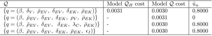
We tested whether the immune response to BK virus infection and donor kidney in renal transplant recipients could be more accurately described estimating six versus five parameters, using the model found in previous work. Based on our sensitivity analysis in [6], we felt we could reliably estimate 5 parameters including QH = {β, ρ¯EV, δEV, δEK, ρ¯EK}. We chose an additional sixth parameter to estimate to form Q and

ran the corresponding inverse problems. Here we refer to the case of estimating 5 parameters as “Model QH” and the case associated with 6 estimated parameters as “ModelQ”. To estimate the parameters in

Q ModelQH cost ModelQcost uˆn {q= (β, δV, ρ¯EV, δEV, δEK, ρ¯EK)} 0.0031 0.0030 0.8000 {q= (β, ρ¯EV, δEV, δEK, ρV, ρ¯EK)} - 0.0031 0 {q= (β, ρ¯EV, δEV, δEK, λC, ρ¯EK)} - 0.0030 0.8000 {q= (β, ρ¯EV, δEV, δEK, ρ¯EK, ϵI)} - 0.0030 0.8000

Table 8: Ordinary least squares costs and model comparison test statistics for the BK virus models. Model QH is the case in which we estimate 5 parameters and ModelQis the case in which we estimate 6

param-eters. We used the statistical model comparison techniques given above to test whether the OLS cost was significantly lower for Model Q. The resulting model comparison test statistics were not significant at the 95% level, indicating that estimating 6 parameters does not yield a statistically better data fit.

5.3

Comparison of 4 vs. 5 Parameters

We tested whether the immune response to BK virus infection and donor kidney in renal transplant recipients could be more accurately described estimating five versus four parameters, using the model found in [6]. We began with 5 parameters, specifically Q={β, ρ¯EV, δEV, δEK, ρ¯EK}. Then we fixed one out of the five

parameters inQand ran inverse problems involving a four parameter setQH ⊂ Q. We refer to this case as

“ModelQH” and the case associated with 5 estimated parameters as “ModelQ”. We obtained the results

shown in Table 9.

QH ModelQH cost ModelQcost uˆn {q= (β, δEV, δEK, ρ¯EK)} 0.0032 0.0031 0.7742 {q= (β, ρ¯EV, δEK, ρ¯EK)} 0.0033 - 1.5484 {q= (β, ρ¯EV, δEV, ρ¯EK)} 0.0035 - 3.0968 {q= (β, ρ¯EV, δEV, δEK)} 0.0033 - 1.5484

Table 9: Ordinary least squares costs and model comparison test statistics ˆun for the BK virus models.

ModelQH is the case in which we estimate 4 parameters and ModelQ is the case in which we estimate 5

parameters. We again used the statistical model comparison techniques to test whether the OLS cost was significantly lower for Model Q. The resulting model comparison test statistics were not significant at the 95% level, indicating that estimating 5 parametersdoes notyield a statistically better data fit.

6

Concluding Remarks

Acknowledgments

This research was supported in part by grant number NIAID R01AI071915-10 from the National Institute of Allergy and Infectious Diseases, in part by the Air Force Office of Scientific Research under grant number AFOSR FA9550-12-1-0188, and in part by the National Science Foundation under Research Training Grant (RTG) DMS-1246991. The authors are grateful to Dr. S. Prigent for providing the data used in Section 3.

References

[1] B.M. Adams, H.T. Banks, M. Davidian, and E.S. Rosenberg, Model fitting and prediction with HIV treatment interruption data, Center for Research in Scientific Computation Technical Report CRSC-TR05-40, NC State Univ., October, 2005;Bulletin of Math. Biology,69(2007), 563–584.

[2] H.T. Banks, R. Baraldi, K. Cross, K. Flores, C. McChesney, L. Poag, and E. Thorpe, Uncertainty quantification in modeling HIV viral mechanics, CRSC-TR13-16, N. C. State University, Raleigh, NC, December, 2013;Math. Biosciences and Engr., submitted.

[3] H.T. Banks, A. Cintron-Arias and F. Kappel, Parameter selection methods in inverse problem formula-tion, CRSC-TR10-03, N.C. State University, February, 2010, Revised, November, 2010; in Mathematical

Modeling and Validation in Physiology: Application to the Cardiovascular and Respiratory Systems,(J.

J. Batzel, M. Bachar, and F. Kappel, eds.), pp. 43 – 73, Lecture Notes in Mathematics Vol. 2064, Springer-Verlag, Berlin 2013.

[4] H.T. Banks, M. Davidian, S. Hu, G.M. Kepler, and E.S. Rosenberg, Modeling HIV immune response and validation with clinical data, Journal of Biological Dynamics,2(2008), 357–385.

[5] H.T. Banks and B.G. Fitzpatrick, Statistical methods for model comparison in parameter estimation problems for distributed systems,Journal of Mathematical Biology,28 (1990), 501-527.

[6] H.T. Banks, S. Hu, K. Link, E.S. Rosenberg, S. Mitsuma, and L. Rosario, Modeling immune response to BK virus infection and donor kidney in renal transplant recipients, CRSC Technical Report CRSC-TR14-09, NCSU, June 2014; J. Inverse Problems in Science and Engineering, submitted.

[7] H.T. Banks, S. Hu and W.C. Thompson,Modeling and Inverse Problems in the Presence of Uncertainty, Taylor/Francis-Chapman/Hall-CRC Press, Boca Raton, FL, 2014.

[8] H.T. Banks and K. Kunisch, Estimation Techniques for Distributed Parameter Systems, Birkhauser, Boston, 1989.

[9] H.T. Banks and H.T. Tran, Mathematical and Experimental Modeling of Physical and Biological

Pro-cesses, CRC Press, New York (2009).

[10] Kenneth P. Burnham and David R. Anderson,Model Selection and Multimodal Inference(2nd edition), Springer, New York, 2002.

[11] W.H. Day, C.R. Baird and S.R. Shaw, New native species of peristenus parasitizingLygus hesperus in Idaho: Biology, importance and description,Ann. Entomol. Soc. Am.,92(3)(1999), 370-375.