Minimum-Fuel Hidden -Layer Heuristic for Waypoint Navigation of Small-Class UAV.

ABSTRACT

XU, DAHAN. Minimum-Fuel Hidden-Layer Heuristic for Waypoint Navigation of Small-Class UAV. (Under the direction of Dr. Lawrence Silverberg).

Minimum-Fuel Hidden -Layer Heuristic for Waypoint Navigation of Small-Class UAV

by Dahan Xu

A thesis submitted to the Graduate Faculty of North Carolina State University

in partial fulfillment of the requirements for the degree of

Master of Science

Mechanical Engineering

Raleigh, North Carolina 2018

APPROVED BY:

_______________________________ _______________________________ Lawrence Silverberg Andre Mazzoleni

Committee Chair

ii

BIOGRAPHY

Dahan Xu takes his master’s study in mechanical engineering at North Carolina State University from August 2017 to December 2018, mainly focusing on dynamics and relevant simulations. This thesis is based on his graduate research under the instructions of Dr. Lawrence Silverberg. The research is simulation-based and hopefully it will be of help in the UAV

iii

TABLE OF CONTENTS

LIST OF TABLES ... iv

LIST OF FIGURES ... v

Chapter 1 Introduction ... 1

1.1 Overall Background ... 1

1.2 Waypoint Navigation Algorithm ... 2

Chapter 2 Method ... 4

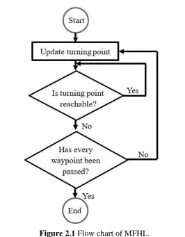
2.1 Flow Chart ... 4

2.2 Illustration with an Example ... 5

2.3 Geometry... 7

2.4 Construct the Optimization Problem ... 9

2.5 Updating Criterion ... 11

2.6 Parameterization ... 12

Chapter 3 Results ... 14

3.1 Results Comparisons for No Disturbance Cases ... 14

3.2 Weight of the Arc Sections During Calculations ... 15

3.3 Results Comparisons with Disturbances ... 16

Chapter 4 Summary ... 19

References ... 20

iv

LIST OF TABLES

Table 2.1 Location of the end points of the first line segment ... 10

Table 2.2 Location of the starting point of the second line segment ... 11

Table A.1 Coefficients for Boundary #1 ... 21

Table A.2 Coefficients for Boundary #1 ... 21

v

LIST OF FIGURES

Figure 1.1 Typical conditions where the waypoints are not reached ... 3

Figure 2.1 Flow chart of MFHL ... 5

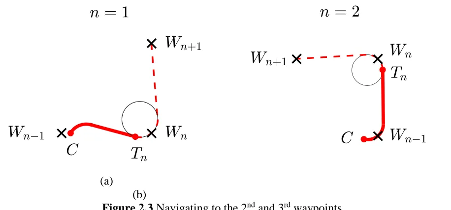
Figure 2.2 Set up of a 6-waypoint example ... 6

Figure 2.3 Navigating to the 2nd and 3rd waypoints ... 6

Figure 2.4 Set up of the coordinate system ... 8

Figure 2.5 Different directions of turning ... 9

Figure 2.6 Geometry for the CW-CCW case ... 9

Figure 2.7 Examples of reachable and unreachable points ... 12

Figure 2.8 Distributions of different turning conditions ... 14

Figure 3.1 WN with and without the MFHL under no disturbances ... 15

Figure 3.2 Example of a CCW-CCW condition ... 16

Figure 3.3 Parameters for the controller ... 17

1

CHAPTER 1

Introduction

1.1

Overall Background

The user community of unmanned systems has been growing significantly. The commercial market net worth reached a reported $8.3 billion in 2018 [1]. We find the largest growth in the commercial markets, in small-class (under 55 pounds) vehicles, in particular. This paper develops an algorithm for a subset of this class of UAV, in particular, for fixed-wing vehicles. Users of small-class UAV are presently navigating autonomously by open-source algorithms such as Missionplanner, Cape, and Pix4D. These navigational systems employ waypoint navigation (WN), wherein the user enters waypoints, whether a priori (static) or not (dynamic). The practice of WN in this community is a constraint to which development work adheres. The community is growing, and with that, demanding higher performance. In RC flight, the racing community requires more precise path following and the growth in autonomous flight is expected to demand greater precision in path following resulting from its applications.

2

1.2

Waypoint Navigation Algorithm

The WN algorithm guides the vehicle in straight-line paths between waypoints. The feedback control has a limit on banking which creates, effectively, a minimum turning radius at a particular flight speed. When approaching a target waypoint, the threshold criterion updates the target waypoint when the vehicle is within a certain radius of it, called the threshold radius. The minimum turning radius and the threshold radius create a trade-off between overshooting the desired path and precisely reaching target points. Due to intermittent wind disturbances, the threshold criterion also results in a tradeoff between reaching the waypoint and missing the waypoint, the latter intermittently resulting in the vehicle turning around to try again and reach the waypoint. Indeed, the threshold criterion, because it is distinct from the smallest desirable turning radius and from wind disturbance considerations, can be difficult to tune, and can lead to undesirable performance. In addition to not reaching a waypoint precisely, the aforementioned problems result in a loss of fuel. Figure 1.1 gives three typical conditions where the performance of traditional WN algorithm can be improved.

(a) (b) (c)

4

CHAPTER 2

Method

This chapter develops the minimum fuel hidden layer (MFHL). The MFHL preserves the waypoint navigation strategy in the foreground (The interface and waypoints specified by the user do not change) but changes the waypoints and the criterion for updating waypoints in the background. The MFHL replaces the traditional threshold criterion with a new criterion that, in effect, gives priority to a minimum turning radius, to reaching the waypoint, and to avoiding missing it – without a trade-off. Toward this end, the MFHL employs the new concept of turning points along with the new criterion for updating turning points based on whether or not a turning point is reachable.

2.1

Flow Chart

The MFHL approaches navigation as an optimization problem within a local optimization space that consists of a current point and two future waypoints. At any instant, the vehicle seeks to reach a turning point that is determined by minimizing fuel along the path up to the second future waypoint constituting the horizon. The trajectory, and hence the optimization problem, is updated once the turning point is unreachable. The reachability condition is determined from the vehicle’s position, heading, and turning radius. For the purposes of real-time implementation, the trajectory may be updated more frequently than when the turning point is updated (like under the conditions of high winds). The stated optimization problem yields desired paths that are

5

2.2

Illustration with an Example

To illustrate the MFHL, consider the 6-waypoint navigation problem shown in Figure 2.2. We will first treat the disturbance-free and error-free navigation problem, that is, the ideal navigation problem, followed by navigation in the presence of disturbances. The former focuses on the navigation part of the problem and the latter on performance in the presence of

disturbances (feedback).

6 Referring to Figures 2.2 and 2.3, the vehicle starts at 𝑊₀ and heads to 𝑊₁. At this point, the MFHL is considering waypoints W0, W1, and W2. The other points are beyond the horizon. Figure 2.3 shows the paths from W0 to W2 (top drawing) and from W1 to W3 (bottom drawing).

As shown, T1 denotes the turning point associated with W1. It lies on the line tangent to a turning circle that has a turning radius R. The turning radius is the minimum turning radius specified by the user. The optimization problem minimizes the fuel from W0 around and touching

W1 to W2. The orientation of the turning circle is free to rotate about W1so the optimization problem is a minimization problem of fuel expressed in terms of the turning circle’s orientation.

Figure 2.2 Set up of a 6-waypoint example.

(a) (b)

7 The fuel consumed during a turn is greater than the fuel consumed while flying in a straight line over the same distance. Typically, the fuel can be as much as 40% greater when turning than when following a straight line depending on turning radius, speed, and vehicle type. Even though the minimization is over the distance extending to W2, the MFHL updates the vehicle’s path once

it reaches point T1. Thus, the vehicle does not follow the section of the path from T1 to W2; the MFHL recalculates that section of the path in the next iteration. Under ideal conditions, MFHL updates the planned path when the vehicle crosses T1, at which point T1 is determined to be unreachable. Under real conditions, disturbances result in the vehicle not reaching point T1 precisely. Point T1 is determined to be unreachable at a point C that is different but close to T1. Referring to the right drawing, the new horizon is set to W3 and the new turning point T2 is determined from the vehicle’s current point C and current direction of flight and the locations of points W2 and W3. As shown, the optimization problem now minimizes the fuel from C around and touching W2 to W3. The optimization problem is now a minimization problem of fuel from C

to W3expressed in terms of the new turning circle’s orientation The MFHL updates the iterations until the vehicle reaches its last waypoint.

2.3

Geometry

In order to derive a closed-form solution for the path planning, we have to construct a coordinate system involving the vehicle and the waypoints and identify the key parameters. For the nth iteration, the vehicle is heading to Wn. A coordinate system was set up so its x-axis points

from C to Wnand its y-axis is perpendicular to x in the direction of Wn+1. The data is scaled such

8 radius R; equivalently R = 1. We perform all the calculations after the geometric parameters are normalized with respect to R. The system is shown in Figure 2.4.

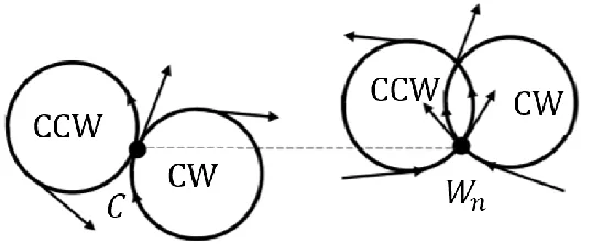
As shown,  is the heading angle (between –1800 and 1800) and  is the turn angle (between 0 and 900₎1_{. At point C, the vehicle turns counter-clockwise (CCW), or clockwise} (CW). Likewise, it turns around Wn CCW or CW. In total, there are four cases: CCW-CCW,

CCW-CW, CW-CCW, and CW-CW. The minimum fuel solution is calculated for each case and the smallest of them yields the true minimum (See Figure 2.5).

1 _{The x axis, because it is along the line through C and W}

n, can cause  to exceed 900.

Figure 2.4 Set up of the coordinate system.

9

2.4

Construct the Optimization Problem

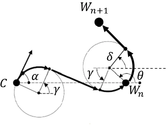
Figure 2.6 shows the geometry of the CW-CCW case. The fuel from C to Wn+1 is a

function of the orientation angle  of the turning circle. (The other cases, not shown, are similar.) The fuel is Fu = waLa +wsLs where Lais the length of the two arcs, Ls is the length of the two

straight segments, and wa and ws are corresponding weights. Letting wa = ws = 1, yields the

minimum distance problem: L = La +Ls. In the results section, we will show that the minimum

distance and minimum fuel solutions are nearly indistinguishable under a broad range of

conditions, allowing the minimum distance solution to approximate the minimum fuel solution. This is important because the minimum distance solution is independent of the vehicle’s

properties. This increases the versatility of the MFHL and ease of implementation.

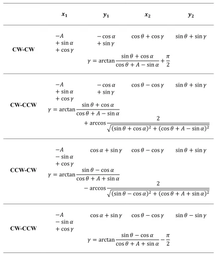
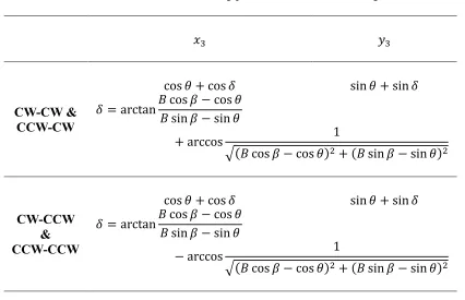
Referring again to Fig. 6, the first straight line segment starts at tangential point (x1, y1) and ends at turning point Tn = (x2, y2). The second line segment starts at tangential point (x3, x4).

Note that we define the first circle by the current position C and the vehicle’s heading; it is either CCW or CW. The location of the second circle depends on the orientation angle . The second

10 line segment is tangent to the second circle and passes through Wn+1 and therefore is uniquely

expressed in terms of the angle  shown, which, in turn, depends on . The coordinates x1, y1, x2,

y2, x3, and y3 for each of the four cases are given in Table 2.1 and Table 2.2.

Table 2.1 Location of the end points of the first line segment.

𝒙𝟏 𝒚𝟏 𝒙𝟐 𝒚𝟐

CW-CW

−𝐴 + sin 𝛼 + cos 𝛾

− cos 𝛼 + sin 𝛾

cos 𝜃 + cos 𝛾 sin 𝜃 + sin 𝛾

𝛾 = arctan sin 𝜃 + cos 𝛼 cos 𝜃 + 𝐴 − sin 𝛼+

𝜋 2

CW-CCW

−𝐴 + sin 𝛼 + cos 𝛾

− cos 𝛼 + sin 𝛾

cos 𝜃 − cos 𝛾 sin 𝜃 + sin 𝛾

𝛾 = arctan sin 𝜃 + cos 𝛼 cos 𝜃 + 𝐴 − sin 𝛼

+ arccos 2

√(sin 𝜃 + cos 𝛼)2_{+ (cos 𝜃 + 𝐴 − sin 𝛼)}2

CCW-CW

−𝐴 − sin 𝛼 + cos 𝛾

cos 𝛼 + sin 𝛾 cos 𝜃 − cos 𝛾 sin 𝜃 + sin 𝛾

𝛾 = arctan sin 𝜃 − cos 𝛼 cos 𝜃 + 𝐴 + sin 𝛼

− arccos 2

√(sin 𝜃 − cos 𝛼)2_{+ (cos 𝜃 + 𝐴 + sin 𝛼)}2

CW-CCW

−𝐴 − sin 𝛼 + cos 𝛾

cos 𝛼 + sin 𝛾 cos 𝜃 − cos 𝛾 sin 𝜃 − sin 𝛾

𝛾 = arctan sin 𝜃 − cos 𝛼 cos 𝜃 + 𝐴 + sin 𝛼−

11

Table 2.2 Location of the starting point of the second line segment

𝑥3 𝑦3

CW-CW & CCW-CW

cos 𝜃 + cos 𝛿 sin 𝜃 + sin 𝛿

𝛿 = arctan𝐵 cos 𝛽 − cos 𝜃 𝐵 sin 𝛽 − sin 𝜃

+ arccos 1

√(𝐵 cos 𝛽 − cos 𝜃)2_{+ (𝐵 sin 𝛽 − sin 𝜃)}2

CW-CCW & CCW-CCW

cos 𝜃 + cos 𝛿 sin 𝜃 + sin 𝛿

𝛿 = arctan𝐵 cos 𝛽 − cos 𝜃 𝐵 sin 𝛽 − sin 𝜃

− arccos 1

√(𝐵 cos 𝛽 − cos 𝜃)2_{+ (𝐵 sin 𝛽 − sin 𝜃)}2

By appropriately manipulating the geometric relationships, the path length (the objective function) becomes a function of the orientation angle  of the turning circle.

2.5

Updating Criterion

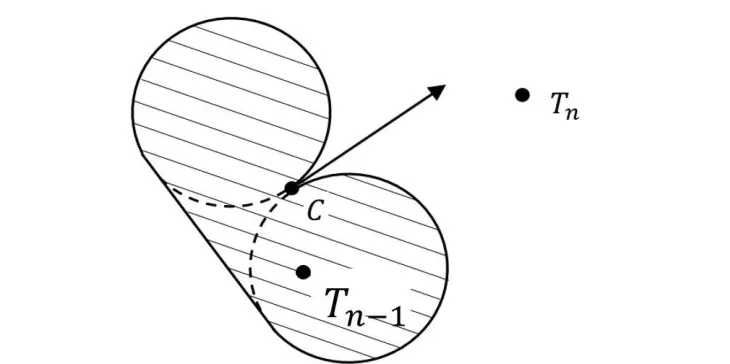
As described earlier, the MFHL guides a vehicle to a waypoint until it becomes

unreachable, at which point it updates the waypoint. Fig. 2.7 shows the reachability condition. As shown, a reachability area consists of CCW and CW circles “enclosed” on the rear by a tangent line. At this time instance, the point 𝑇_𝑛−1 is already inside the shaded area so it is determined to be “unreachable”. Consequently, point 𝑇_𝑛−1 is omitted and the vehicle is being navigated to Tn. At any given instant of time, Tncould be either inside or outside the reachability

12 as it is inside the reachability area, Tn becomes unreachable, and the MFHL updates the waypoint

to Tn+1.

Note that the purpose of “enclosing” the CCW and CW with the line segment was to prevent the possibility that the two circles pass Tn undetected, which would otherwise be possible because the detection is not truly performed continuously but only at discrete instances of time.

2.6

Parameterization

Clearly, we formulated the 3-point horizon optimization problem to keep the

computational effort minimal for real-time implementation. To further reduce computational effort and for robustness, we parameterized the solution, effectively reducing it to a look-up table. Toward this end, we determined the orientation angle  of a turning circle as a function of the four parameters A, B,  and . For each of the four cases pertaining to turning CW and CCW, the orientation angle is a continuous function of the four parameters. Discontinuities, however, arise when transitioning from one case to another. Thus, we parameterized the

13 orientation angle by smoothly fitting the data to the four parameters separately for each case. Toward distinguishing between the different cases, we needed to parameterize the boundaries of each of the cases in terms of the four parameters. In particular,  and  transition from case to case due to changes in A and B. For example, consider the graph of  versus  shown in Fig. 2.8 for particular parameters (A = B = 4, wa = ws = 1).

As shown, there are three boundaries and three interior regions. (The CW-CW case never produces an optimal orientation angle.) We express the boundary of the turn angle  as a

function of the heading angle  in which its coefficients are expressed as a function of the distances A and B :

2

0 1 2 1 2

2

0 2 1

1 2 2 /2 4 /2 4

a a a a a

a a a

a a a  +  +    −   =_{ −}   −   2 2

0 1 2 3 4 5 ( 1, 2, 3)

i i i i i i i

a =b +b A b A+ +b B b B+ +b AB i=

14 We determined the coefficients b0i through b6i (i = 1, 2, 3) separately for each of the

cases (See Appendix).

CHAPTER 3

Results

Let us continue with the 6-waypoint example and compare the current WN problem with and without the MFHL. In the WN problem, navigation performance depends on the minimum turning radius and the threshold radius. With the MFHL, navigation performance depends on minimum turning radius alone. Feedback control is the same whether or not the WN problem employs the MFHL. However, the resulting overshoots differ.

3.1

Results Comparisons for No Disturbance Cases

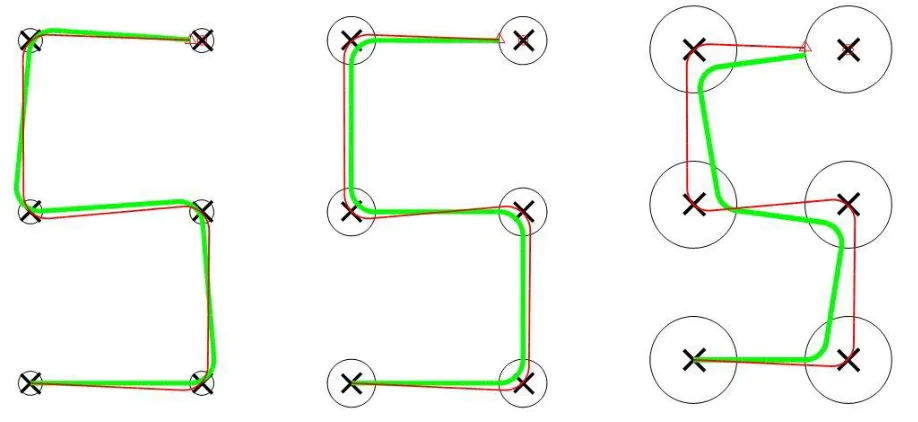
Figure 3.1 compares WN with and without the MFHL. The minimum turning radius R of the vehicle is the same in each of the cases. We see three cases that differ by the waypoint circles. The waypoint circles are 0.5R, R, and 2R, respectively.

15 In each case, there are no disturbances. With the MFHL, the vehicle passes through the waypoints exactly and follows the minimum fuel paths by design. With the standard WN, none of the vehicles reach their waypoints. The vehicle overshoots the desired path when the waypoint radius is less than R. The vehicle follows close to the desired path when the waypoint radius is equal to R, and the vehicle undershoots the desired path when the waypoint radius is larger than

R.

3.2

Weight of the Arc Sections During Calculations

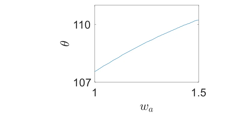
The question arises as to the differences between the minimum fuel and minimum distance solutions, the latter determined when wa = ws = 1. When the distances A and B are very

large compared to the turning radius R, the vehicle is flying in a straight line most of the time and the difference between the two solutions will be very small. The distances tend to be at least four times larger than the turning radius and the expected differences between the two solutions largest in these cases. Figure 3.2 shows a typical example. As shown, the orientation angle of the turning circle does not change more than 40 in this worsted case. In that the penalty of not

16

3.3

Results Comparisons with Disturbances

To illustrate the effect that feedback corrections have on path following, we first constructed a simplified feedback controller and then performed the comparisons with the

simplified controller. Figure 3.3 shows a vehicle at an instant in time heading in a given direction and a reference line with endpoints that are waypoints in the case of standard WN and that are target points when the MFHL is used. The vehicle’s turning angle,  = T+ R, consists of two

parts: the target component T toward the target and the reference part R toward the reference

line. Also shown, the distance between the vehicle and the reference line is denoted by s. The target component of the turning angle is determined from geometry and the reference part from

the feedback law _R T

T

gs hs 

 = +



17 where g and h are control gains and the term T/T dictates the direction of 𝜙_𝑅. Figure 3.4 shows WN with and without the MFHL, both employing the simplified controller and

influenced by a randomly generated disturbance. The minimum turning radius was r = 0.7, the time step was 0.02, the vehicle speed was v = 0.8, and the control gains were g = 0.1 and h = 5.25. With these parameters the turning radius was 0.7.

From Figure 3.4 we can observe similar patterns as from Figure 3.1. The red lines which represent navigation with MFHL always hit the waypoints while the green lines, which represent navigation without MFHL tends to deviate from the waypoints and cost more fuels. It is

Figure 3.3 Parameters for the controller.

19

CHAPTER 4

SUMMARY

In the growing class of small-class unmanned aerial vehicles, waypoint navigation suffers from an existing trade-off between minimum turning radius and threshold radius that prevents vehicles from reaching waypoints and closely following desired paths. This paper developed an algorithm, called the minimum-fuel hidden layer (MFHL) that remedies this problem in a way that is invisible to the user. The paper showed how, by establishing a horizon that includes two future waypoints, to improve the performance of WN in terms of fuel and time. For real-time implementation, we reduced the computational effort, essentially eliminated it, by

20

References

[1] Drubin, Cliff. UAV Market Worth $8.3 B by 2018. Microwave Journal, International ed.; Dedham Vol. 56, Iss. 8, (Aug 2013): 37.

[2] Bakolas, Efstathios and Tsiotras, Panagiotis. Feedback Navigation in an Uncertain Flow Field and Connections with Pursuit Strategies. Journal of Guidance, Control, and Dynamics, Vol. 38, No. 4 (2015), pp. 631-642.

22

Curve Fitting for the Boundaries in

𝛼 − 𝛽

Plane

Boundary #1:

Table A.1 Coefficients for Boundary #1.

𝑎₀ 𝑎₁ 𝑎₂

𝑏1 -360853 4010.94 -11.15

𝑏 126331.6 _{-1398.93 3.87}

𝑏₃ -14947.5 _{166.36 -0.46}

𝑏4 3826.06 -42.05 0.12

𝑏5 587.91 -6.57 0.02

𝑏₆ -2448.85 _{27.29 -0.08}

Normalized % error*

7.16 7.12 7.08

Boundary #2:

Table A.2 Coefficients for Boundary #2.

𝑎₀ 𝑎₁ 𝑎₂

𝑏₁ 23.9 20.98 8.4

𝑏₂ -1.63 -11.9 -2.59

𝑏₃ 0.16 0.51 0.1

𝑏4 -0.39 -1.12 -0.34

𝑏5 0.01 0.05 0.02

𝑏₆ 0.02 -0.002 0.002 Normalized

% error*

23 Boundary #3:

This boundary is calculated explicitly:

𝛾 = arctan cos 𝛿

−𝐴 − sin 𝛿+ arcsin

1

√cos2_{𝛿 + (𝐴 + sin 𝛿)}2

Curve Fitting for

𝜽

𝜃 = 𝑓(𝐴, 𝐵, 𝛼, 𝛽)

Table A.3 Coefficients for calculating 𝜃.

Term CW-CCW CCW-CW CCW-CCW

1 1.3918 -1.4939 1.6151

A 0.0221 -0.0089 -0.0088

B -0.0039 0.0025 0.0082

A2 _{-0.0007 0.0003 0.0003}

B2 _{0.0002 -0.0001 -0.0003}

1/A 0.7966 -0.4697 -0.5436

1/B -0.1017 0.0415 0.1253

 0.6679 -0.4009 0.4802

 -0.0272 0.0819 0.0096

 0.0088 0.052 -0.0098

24

Table A.3 (Continued).

_{ -0.0004 -0.002 0.0004}

 -0.6481 1.3486 0.3613

 0.1841 0.9679 -0.2026

 0.288 0.1453 0.0964

A -0.031 -0.0162 -0.0122

B 0.0039 0.0053 0.0081

A2_{ 0.001 0.0005 0.0004}

B2_{ -0.0002 -0.0002 -0.0003}

 -1.5572 -1.1682 -1.116

 0.1043 0.1066 0.1111

 _{-0.0897 -0.4233 -0.0141}

A _{0.013 0.1502 -0.0037}

B _{-0.0025 -0.0495 0.0063}

A2 _ _{-0.0004 -0.0077 0.0001}

B2_ _{0.0001 0.0014 -0.0002}

AB _{0 0.0026 0}

_{ 0.2039 1.4862 -0.2467}

_{ 0.0165 -0.5278 0.2181}

 _{-0.0834 0.0306 0.0225}

A _{0.0087 -0.004 -0.0032}

25

Table A.3 (Continued).

A2_ _{-0.0003 0.0001 0.0001}

_{ 0.3168 -0.201 -0.2037}

_{ -0.0215 0.045 0.0416}

 0.0236 -0.3978 -0.0069

A 0.0004 0.0337 0.0002

B -0.0035 0.0262 0.0004

A2_{ 0 -0.0015 0}

B2_{ 0.0001 -0.001 0}

 -0.0083 0.5157 -0.0337

 -0.0537 0.567 0.0419

1/ -0.0001 0 -0.0007

1/(A) 0 0 0.0059

1/(B) 0.0003 0 -0.0016

1/ -0.0001 0.0003 0.0014

A/ 0 -0.0005 -0.0002

B/ 0 0.0006 0

1/(A) -0.0015 -0.0136 -0.006

1/(B) 0.0015 0.0096 0.0013

Normalized % error

0.4021 0.5329 0.3983