A New Method to Evaluate Hydrogen Sulfide Removal from Biogas

ABSTRACT

MARTIN, JERRY HUGHES. A New Method to Evaluate Hydrogen Sulfide Removal from Biogas. (Under the direction of Jay Cheng.)

Hydrogen sulfide in biogas fuel increases the speed at which the system utilizing the biogas

corrodes. This corrosion may be prevented by separating and removing hydrogen sulfide from

the biogas. There are multiple technologies available to remove hydrogen sulfide (such as the

gas-gas membrane tested in this thesis); however, evaluating the effectiveness of hydrogen

sulfide removal in an inexpensive manner is difficult to do.

A device was constructed capable of a virtually simultaneous high precision volumetric flow

and concentration measurements on moving biogas. The volumetric flow was measured by

sampling the pressure from the center of two different points along a rigid tube and correlating

pressure sensor voltage to the maximum velocity measured with a velocity probe. The hydrogen

sulfide and methane concentrations were measured using chemical gas sensors.

A mass balance was completed around a reverse selective membrane system with the

calculated difference between flows based on known input and measured output concentrations

coming within 15% of each other. Though the volumetric flow measurements were in doubt,

this device was able to determine that using a 20 cm2 polyamide membrane under low pressures suitable for a digester (2 PSI) will increase methane concentration in biogas from 60% to 62%

but is not effective at removing hydrogen sulfide.

This device was primarily designed for determining the feasibility of adapting a membrane

system to a farm scale biogas generation process. This device was able to determine that using a

polyamide membrane under low pressures suitable for a digester (2 PSI) will increase methane

concentration in biogas from 60% to 62% but is not effective at removing 1000 ppm of hydrogen

sulfide.

Keywords: Agricultural Waste, Anaerobic Digestion, Animal Wastes, Bioenergy,

Biogas, Energy Recovery, Hydrogen Sulfide, Membrane, Methane, Methane Production,

A New Method to Evaluate Hydrogen Sulfide Removal from Biogas

by

Jerry Hughes Martin II

A thesis submitted to the Graduate Faculty of North Carolina State University

in partial fulfillment of the requirements for the Degree of

Master of Science

Biological and Agriculture Engineering

Raleigh, North Carolina

2008

APPROVED BY:

_________________________ Dr. D. Knappe

____________________ _________________________

Dr. J. Cheng Dr. P. Westerman

ii

DEDICATION

This research is dedicated to Olin and Eloise Epps (my grandparents) who sacrificed to further my education. It is also dedicated to the memory of the late Dr. William Epps

iii

BIOGRAPHY

I was born in Latta, SC. My parents are Jerry Martin (an NCSU graduate) and

Jane Martin. I attended Clemson University and received a bachelor’s degree in

electrical engineering (2003). After a brief period of working in the textile industry as a

process engineer and a manager in charge of a warp-knit product line I began work on a

master’s degree in bioprocess engineering at North Carolina State University.

While at North Carolina State I developed virtual instrumentation for Dr Gary

Roberson to teach the use of a GPS system and yield mapping. I also worked under Dr

Mike Boyette developing wireless controls and monitors for bulk tobacco barns.

Near the completion of this thesis, I accepted a position working as a research

engineer for the USDA-ARS Coastal Plains Research Station in Florence, SC. My

position involves the development of technologies and techniques in finding new uses

for biomass including alternative energy. I am involved in both biological and

thermochemical technologies research.

My research interests are in bio-separations and the use of software modeling,

electronic control, wireless systems and measurement technologies in microbiological

iv

ACKNOWLEDGEMENTS

There are many people who helped contribute to this research.

The original idea for this research came from a class taught by my adviser, Dr. Jay

Cheng. I learned a great deal from him. My advisor and my committee Dr. Philip

Westerman and Dr. Detlef Knappe held this work to high standards and forced me to

push my limits further than I thought they could go.

Dr. Mike Boyette allowed the use of his lab and resources to construct the apparatus.

Deepak Keshwani, along with the rest of Dr. Cheng’s research group, helped in securing

supplies.

Dr. Dan Willits helped while Dr. Cheng was in Bulgaria.

Haiqing Lin from Membrane Technology and Research Inc. donated the membrane and

gave technical assistance in its use.

Marcia Gumpertz and Jessie Zhang from the statistics department helped develop a

statistical model. It was never used because this thesis turned into a methods thesis.

Scott Brigman of Temperance Hill, South Carolina manufactured the membrane holder

at no cost.

Martin Brice from Gas Fired Products provided technical insight into the gas industry.

Cyrus Yunker helped draw up specifications for the volumetric flow sensors.

Micheal Banks from National Specialty Gases helped get the right parts to handle the

v

Harold Morton with the Department of Environmental Health and Safety at NC State

helped make sure this experiment was safe to run.

The building personnel, hazard response team, and firefighters responded quickly when

the fire alarm was pulled. If that had been an actual gas cylinder mishap my life may

have been saved.

Both the branch office of South Carolina Electric and Gas and Lockemy Scrap Metal

located in Dillon SC helped with the material in some of the photos.

Dr. Keri Cantrell from USDA, agriculture research service reviewed part my thesis

before I submitted it. Dr. Ro from the same location showed me how to set up the

calibration curves.

Dr. George Gopen, an English professor from Duke University advised me that the most

important sentence in the entire thesis was the last sentence in the first (or first group) of

paragraphs. The same held true for every chapter and section. His book was helpful too.

It had his research into how to produce good technical writing.

My father and mother, Jerry and Jane Martin, edited my thesis for grammatical errors.

To my parents, grandparents, and my church community I express my thanks for their

vi

TABLE OF CONTENTS

LIST OF FIGURES. . . viii

LIST OF TABLES. . . ix

CHAPTER 1 Introduction . . . 1

CHAPTER 2 A Literature Review of Hydrogen Sulfide in Biogas . . . 3

2.1 Introduction . . . 3

2.1.1 Composition of Biogas. . . 3

2.2 The Issue with Hydrogen Sulfide . . . . . . 7

2.2.1 The Corrosion Phenomena . . . 8

2.3 Methods for Eliminating Hydrogen Sulfide . . . . . . 12

2.3.1 Altering Anaerobic Digestion/Energy Cogeneration Process . . . . 14

2.3.2 Removing the Sulfur from Feed and Washwater . . . 15

2.3.3 Direct Treatment of Biogas . . . 16

2.4 Conclusion . . . 17

CHAPTER 3 A New Method for Detecting Hydrogen Sulfide Concentration in Biogas . . . . 18

3.1 Introduction . . . 18

3.1.1 Detecting Concentrations of Methane . . . . . . 18

3.1.2 Detecting Concentrations of Hydrogen Sulfide . . . . . 19

3.2 Materials . . . 19

3.2.1 Gas Sensors . . . . . . 20

3.2.2 Volumetric Flow Sensors . . . 22

3.3 Methods . . . . . . 27

3.4 Results . . . 27

3.5 Conclusion . . . 33

CHAPTER 4 Testing Biogas Passed Through a Gas-Gas Membrane System for Hydrogen Sulfide Removal . . . 34

4.1 Introduction . . . 34

4.2 Theory . . . . . . 35

4.2.1 Selectivity Mechanisms . . . 35

4.3 Materials . . . . . . 39

4.4 Methods . . . . . . 44

vii

4.6 Conclusion . . . 53

BIBLIOGRAPHY. . . 55

APPENDICES . . . . . . . . . . . . . . . 60

APPENDIX A History of Biogas . . . 61

APPENDIX B Biogas Safety . . . 62

B.1 Explosion . . . 62

B.2 Asphyxiation . . . . . 62

B.3 Hydrogen Sulfide Poisoning . . . 63

B.4 Infection from Swine Wastes . . . 63

APPENDIX C Extended Explanation for Diagrams . . . 64

C.1 The Derivation of the Potential - pH Diagram . . . 64

C.2 The Volumetric Flow Signal Conditioning Circuit . . . 65

APPENDIX D Software . . . 67

APPENDIX E Another Membrane Configuration? . . . 72

viii

LIST OF FIGURES

Figure 2.1 Breakdown of Organics into Biogas . . . 5

Figure 2.2 Location in Cylinder Liner Where Corrosion Forms . . . 8

Figure 2.3 Corrosion in Metal Showing Where Droplets of Electrolyte Formed . 9 Figure 2.4 Pitted Anoxic Corrosion . . . 11

Figure 2.5 Corrosion Phenomena in the Methane/Biogas-Iron System . . . 13

Figure 3.1 Hydrogen Sulfide Sensor . . . 20

Figure 3.2 Diagram of the Potentiostat . . . 20

Figure 3.3 Methane Sensor . . . 22

Figure 3.4 Circuit to Drive Methane Sensor . . . 22

Figure 3.5 Volumetric Flow Sensing System . . . 23

Figure 3.6 The Low Electrical Noise in the Pressure Sensing Circuit . . . 26

Figure 3.7 Signal Conditioning Circuitry . . . . . . . . . . 27

Figure 3.8 Graph Comparing the Voltage of the Pressure Sensor Circuit to Maximum Velocity Over a Series of Flow Step Increases . . . 28

Figure 3.9 The Linear Relationship between the Maximum Velocity and Pressure Sensor Voltage . . . 29

Figure 3.10 The Signal Given When the Flow Changes from a Steady Flow of Air to a Diluted Flow . . . 30

Figure 3.11 The Voltage Signals from the Gas Sensors when a Forty-Five Second Pulse of Biogas was added to the Diluted Flow . . . 31

Figure 3.12 The Concentration versus the Flow Sensor Voltages . . . 31

Figure 3.13 The Concentration Regressed on the Flow Sensor Voltage . . . 32

Figure 4.1 The Molecular Shapes of Component Gases in Biogas . . . 36

Figure 4.2 An Exploded View of the Membrane Holder with the Membrane in it 40 Figure 4.3 Pressurized Chamber Mounted on the Membrane Holder . . . 41

Figure 4.4 Gas Sensors Mounted on the Apparatus . . . 42

Figure 4.5 Close-up of Mechanisms Attached to Membrane Holder . . . 43

Figure 4.6 Complete Apparatus . . . 44

Figure 4.7 Diagram Showing Flows Through the Membrane . . . 45

Figure 4.8 Thermal Correction Curve Superimposed on the Raw Voltage Curve from Flow Sensor . . . 50

Figure 4.9 Calculation of the Input Concentrations Based on the Output Concentrations over Time . . . 51

Figure E.1 Membrane Hanging Out Side of Holder. . . 73

Figure F.1 The Setup Used to Verify the Flow Measurement . . . 75

Figure F.2 Comparing the Velocity Measurement in the Experiment to a Second Velocity Measurement Technique. . . 76

ix

LIST OF TABLES

1

CHAPTER 1

Introduction

This research addresses three economic needs of North Carolina. The first is

treating wastes from the economically important swine industry, the second is for

alternative fuel sources that are inexpensive, and the third is for preserving capital

investments in energy conversion technologies from damage caused by sulfide

corrosion.

The importance of the swine industry can be highlighted using 2004 North

Carolina agricultural commodities statistics. During that year the North Carolina swine

industry generated two billion dollars which accounted for over one quarter of the total

revenue brought in by sale of North Carolina agricultural

commodities (NCDACS, 2004). To get this revenue North Carolina housed ten million

swine that excreted an estimated seven million tons of waste. Traditionally, this waste

was handled using treatment system that included an open lagoon; however, a recently

enacted law in North Carolina (NC law # 2007-523) has prohibited new lagoon

construction. This law will force farmers to explore and improve already existing

alternatives to treatment systems involving open lagoons. One of the alternatives being

considered is anaerobic digestion technologies.

Anaerobically digesting swine manure is a waste management alternative with a

benefit of the generation of biogas fuel. Using biogas in place of natural gas will help a

farmer avoid having to buy as much gas on the open market. This protects farmers from

the escalation of and volatility in natural gas prices (Wiser and Bolinger, 2007).

Most energy generation systems built to utilize biogas are constructed from

metals or plastics that are vulnerable to sulfide damage. The damage to these systems

begins to occur when hydrogen sulfide in biogas exceeds 100 ppm. This damage

2

must be removed so having a good, inexpensive analytical test to determine the

concentration and flow of hydrogen sulfide in the biogas will speed the development of

better methods for reducing sulfide in biogas. This research addresses the sulfide

problem by introducing a means to quickly test the effectiveness of methods that reduce

the concentration of hydrogen sulfide in biogas. Having better methods for reducing

biogas corrosion is likely to become more important in the coming years, especially in

systems that use metals such as copper, zinc, nickel, tin, platinum, and their alloys since

the supply of ore for these metals are limited (Gordon, Bertram and Graedel, 2006).

The goal of this thesis is to present an analytical technique for evaluating how

well technologies work for removing hydrogen sulfide from biogas. This technique is

applied to a selective gas-gas membrane system that works by pushing hydrogen sulfide

through a membrane, but not methane.

The next chapter of this thesis is intended to present a thorough background of

corrosion caused by biogas and current alternatives for removing hydrogen sulfide. The

third chapter contains a detailed description of the development of a new analytical

technique for detecting the flow and concentration of the gases in biogas. The final

chapter is an analysis on a system that has the potential to effectively reduce the

3

CHAPTER 2

A Literature Review of Hydrogen Sulfide in Biogas

2.1

Introduction

Converting wastes into biogas is a way to recover energy from the waste, to

reduce odors, to increase nutrient availability, and to reduce pathogen content (Garrison

and Richard, 2005; Goodrich and Schmidt, 2002). While converting waste to biogas is

desirable, one of the reasons it is not common is because of the poor quality of biogas

and the high maintenance requirement of biogas using systems (Stowell

and Henry, 2003). Removing hydrogen sulfide from the biogas or sulfur from any point

in the biogas generation process would take care of both of these issues.

2.1.1

Composition of Biogas

Table 2.1 shows the concentration of hydrogen sulfide in biogas, as well as the

concentrations of other major component gases, carbon dioxide and methane. Landfill

biogas does not have as much hydrogen sulfide in it because the organic materials

decompose several years while manures are digested fresh (KiHyun et al., 2005).

Table 2.1: Composition of Various Forms of Biogas

Substrate (by

volume)

H

S

CO

CH

(Pagilla, Kim

and Cheunbarn, 2000) Cattle Manure 600 - 7000 40 60 (Bothi, 2007)

Landfill Wastes 0 - 2000 30 - 50 50 - 70 (Shin et al., 2002)

Biogas from manure is generated biologically by anaerobic digestion of the

complex organic molecules. Under anaerobic conditions microorganisms break down

4

oxidized state (Kotelnikova, 2002). Roughly sixty percent of the carbon is reduced and

volatilizes as methane while the rest of the carbon volatilizes as carbon

dioxide (Angenent et al., 2004).

As many as 138 different microorganisms contribute to the production of biogas

from swine manure with the majority of them being strict anaerobes (Iannotti, et

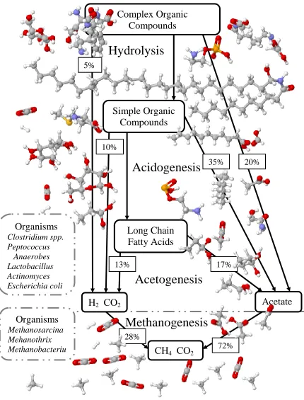
al., 1982). As presented in Figure 2.1, these microorganisms can be broadly classified

into two physiologically distinct groups. The first group breaks down the complex

organics into simpler organic molecules (hydrolytic and fermentor organisms). The

second group uses the simple organic molecules, particularly acetate and hydrogen, to

make methane (methanogenic organisms) (Cappenberg, 1975; Tchobanoglous, et al,

2002).

While manure is being digested, very small bursts of hydrogen sulfide will

bubble out (Ni et al., 2001; Arogo et al., 2000) and accumulate as a small portion of

biogas. Hydrogen sulfide is produced during hydrolysis when certain organisms break

down the essential amino acid methionine (Ravanel et al., 1998; Zhu, et al., 1999). In

the methanogenic stage hydrogen sulfide production continues because a different group

of sulfate reducing organisms can use fatty acids, particularly acetate, as a substrate

5

Figure 2.1: Breakdown of Organics into Biogas

Long Chain

Fatty Acids

CH

CO

Acetate

Simple Organic

Compounds

H

CO

Hydrolysis

Acidogenesis

Acetogenesis

Methanogenesis

Organisms

Clostridium spp. Peptococcus Anaerobes Lactobacillus Actinomyces Escherichia coli

Organisms

Methanosarcina Mehanothrix Methanobacteriu m

Complex Organic

Compounds

10% 5%

20% 35%

17% 13%

6

Sulfate reducers are a nuisance because they grow faster than methanogenic

organisms using the same substrates (Oremland and Polcin, 1982). This was shown

when acetate and sulfate were used to culture a sulfate reducer Desulfobacter postgatei

and a methanogen Methanosarcinabarkeri with similar maximum growth rates,

μmax

fifteen times less than Methanosarcina barkeri’s KS which was 3 mM (Schönheit,

Kristjansson and Thauer, 1982). Acetate concentration in swine manure is around 51

mM (Hansen, Angelidaki and Ahring, 1999) so the growth rate,

μ

μmax

μ

μmax

μ

μmax

μ

As sulfate is reduced hydrogen sulfide is formed, which is another problem

because the hydrogen sulfide byproduct is inhibitory to all organisms involved in

anaerobic digestion (Cypionka, 1986), especially the methanogens (Hulshoff

et al., 1998, Chen et al., 2008).

S

K

S

S











When conversion techniques other than anaerobic digestion are used, hydrogen

sulfide is still a problem. A gas similar to biogas called syngas can be produced from

manure by gasification or pyrolysis using a thermochemical reactor (Chang, 2004).

Thermochemical reactors use more energy than anaerobic digesters, however, they are

more compact and convert the waste much faster (Cantrell et al., 2007). During

thermochemical conversion, syngas is created by heating up the manure in either

7

combination of hydrogen gas and carbon monoxide. This gas can be reformed into

methane and carbon dioxide by passing it through high temperature steam. In

thermochemical reactions free energy changes tend to favor sulfate reduction over

methane formation. Table 2.2 shows the free energies associated with different sulfate

reductions.

Table 2.2: Stoichiometry for Sulfate Reduction and Methanogenisis

Reaction Δ G (kJ/mol)

Sulfate-reducing reactions 4

H

SO

2- ₊

_H

→

_HS

_H

2

O

-

.

Acetate

_SO

42-

→

HS

-

HCO

-

-

.

Propionate

+

SO

2-

→

_HS

+

Acetate

+

HCO

H

-

.

Methanogenic reactions 4

H

HCO

+

H

→

_CH

4 + 3

H

O

-

.

Acetate

+

H

O

→

CH

HCO

-

.

adapted from Lens et al. (1998)

2.2

The Issue with Hydrogen Sulfide

Hydrogen sulfide in biogas is one of the main reasons that the benefits currently

do not outweigh the cost of an anaerobic digester (Garrison and Richard, 2005; Stowell

and Henry, 2003). There are a few cases, such as one dairy waste digester reported

by Goodrich and Schmidt (2002), that had few problems in terms of hydrogen sulfide

damage, but in most cases the damage from the sulfide in the biogas causes equipment

and maintenance costs to increase (Li, 1984; Lusk, 1998). Picken and Hassaan (1983)

explicitly mention engine problems caused by hydrogen sulfide in biogas when it is

8

Biogas from anaerobic digestion is mostly methane. If biogas were pure methane

it would be an excellent choice for a fuel. Methane has a simple structure and is highly

stable, which allows for ease of storage and handling. As an engine fuel it has the

advantages of complete combustion, no dilution of lubricants, better exhaustion

performance, and good anti-knock properties (Jiang, et al., 1989). Biogas, however, is

only sixty percent methane. The remaining forty percent is mostly acid gases (primarily

carbon dioxide) with hydrogen sulfide causing the most problems. When real biogas is

burned as a fuel engines tend to wear out quickly. Picken and Hassaan (1983) have

shown that the first part of a biogas engine to wear out is the cylinder liner at the upper

position of the piston ring (see figure 2.2). Excessive wear in cylinder liners at this

position is caused by the corrosion phenomena (Sudarshan

and Bhaduri, 1983; Goode, 1989).

Figure 2.2: Location in Cylinder Liner Where Corrosion Forms

2.2.1

The Corrosion Phenomena

Corrosion is the degradation of a metal as it is converted from a desired to an

undesired form. All metals corrode at certain electrochemical and thermodynamic

conditions. These conditions depend on the pH, chemical potential, and temperature of

the solution. When corrosion occurs, metal ions dissolve into a solution releasing

Corrosion

Cylinder Liner

9

electrons into the metal that is left. These electrons are conducted through the metal to a

location where the solution, metal, and possibly atmosphere meet. There the electron is

accepted by any oxidizing agent present. In this research the common oxidizing agents

that form stable corrosion compounds with the metal are oxygen and sulfur. As more

metal ions dissolve and are oxidized the parts that are metal will become damaged by

being eaten away or by converting into a material resembling the metal’s

ore (Hamilton, 1985). (See equations 2.2, 2.3, and 2.4) Figure 2.3 shows where droplets

of solution formed on the surface of the metal.

Figure 2.3: Corrosion in Metal Showing Where Droplets of Electrolyte Formed

Anode Region

(Where Electrolyte Droplet Formed)

Cathode Region Cathode

10

Corrosion occurs during normal methane combustion. Assuming standard

conditions, combustion of 1 liter of methane (see equation 2.5) has the potential to

produce 1.4 ml of liquid water and 0.9 liters of carbon dioxide. (In industry standard

units 100 ft3 of methane has the potential to produce 1.0 gallons of liquid water and 91 ft3 of carbon dioxide.) The water produced is an electrolyte and the oxygen is the oxidizing agent needed for corrosion. The carbon dioxide speeds up the corrosion by

making the electrolytic solution more acid which, in turn, speeds up the dissolution of

the metal into ions.

(2.5)

Hydrogen sulfide is oxidized into sulfur dioxide which dissolves as sulfuric acid.

Sulfuric acid, even in trace amounts, can make a solution extremely acidic. Extremely

acidic electrolytes dissolve metals rapidly and speed up the corrosion process. This is

particularly true in high temperatures, such as is the case with the afore mentioned

cylinder liner.

Even if there is no oxygen present, biogas can corrode metal. Hydrogen sulfide

can become its own electrolyte and absorb directly onto the metal to form corrosion.

(Brown, 2004). If the hydrogen sulfide concentration is very low, the corrosion will be

slow but will still occur due to the presence of carbon dioxide. People in the pipeline

industry refer to this type of corrosion as sweet corrosion which is recognized by very

deep pits (Smith, 1993). The mechanism for this reaction is given in equations 2.6-2.8

(López, Pérez and Simison, 2003). If the concentration of hydrogen sulfide in the gas is

greater than 100 ppm, people in the pipeline industry refer to the corrosion as sour

corrosion which is recognized by pits as shown in figure 2.4 (Smith, 1993). This

11

Figure 2.4: Pitted Anoxic Corrosion

The presence of hydrogen sulfide causes metals to become more active.

Describing a metal as active is one of three ways to describe the resistance of a metal to

corrosion given a certain set of thermodynamic conditions. The other two are immune

and passive. Immune metals, for example gold, have natural nobility but are too

expensive for making systems that handle biogas. Passive metals are typically used in

biogas applications. These metals have an oxidized coating that slows corrosion. Active

metals have no resistance to corrosion and will dissolve on contact with an electrolyte.

Anything that makes a metal more active will make it corrode faster.

The potential - pH diagram, also known as a Pourbaix diagram, is a graphical

way to show the effect of hydrogen sulfide on the corrosion of metal parts. Figure 2.5 is

a potential - pH diagram for a biogas - iron corrosion system at standard conditions.

Though metal systems for using biogas are never made of pure iron, the pure iron

system has similar thermodynamics, more simplicity, and more empirical data to back it

up than the carbon-iron (steel) or carbon-chromium-iron (stainless steel) typically used

12

in the construct biogas burning systems. The derivation of this diagram is in appendix

C.1.

Point one in figure 2.5 describes the pH and potential a water droplet would have

in standard conditions for a pure methane-iron system. Adding air to the system shifts

the pH and potential of the water droplet from point one to point two. The speed of

corrosion increases as air is added, but this effect is counteracted because the iron will

become passive, or form a protective oxide coating. The difference between the water

droplet in the iron-methane system and the iron-biogas system is shown by shifting from

point one to point four. This shift causes a slight increase in the speed of corrosion. The

practical scenario for utilizing biogas is a shift from point one to point three, where the

biogas is used and oxygen is present. In this scenario the corrosion is fast and the oxide

coating is not as stable, which causes pits form and drastically reduces the useful life of

13

label Oxygen

H

S

H

S

H

S

H

S

H

S

Figure 2.5: Corrosion Phenomena in the Methane/Biogas-Iron System

2.3

Methods for Eliminating Hydrogen Sulfide

The main problem with hydrogen sulfide is that it speeds up corrosion.

Corrosion of metals occurs naturally in devices that burn methane. Trace amounts of

hydrogen sulfide in the gas makes the corrosion worse. For this reason it is hard to use Normal Fe-CH4 System

add air add H2S

14

biogas to displace natural gas without first removing the hydrogen sulfide. There are

several methods currently available for removing the sulfide gas.

2.3.1

Altering Anaerobic Digestion/Energy Cogeneration Process

Codigestion

Codigestion refers to digesting multiple substrates in a digester simultaneously.

The main benefit of codigestion is the ability of neutralizing two different types of waste

in one digester (Pesta, 2006). There is evidence to suggest adding food wastes to dairy

waste digesters has reduced the concentration of hydrogen sulfide (Bothi, 2007). The

major problem is that both materials must be available at the same site in the right

quantities, which is a rare occurrence. If this is not the case transportation costs may be

involved.

Digester Additions

Iron chlorides, phosphates, and oxides can be added directly to the digester to

bind with the sulfides in the digester and make them insoluble. The addition of iron III

phosphate has been observed to reduce hydrogen sulfide concentration (McFarland

and Jewell, 1989). This solution involves costs of the additions.

Multiple Phase Digestion

Typically, multiple phase digestion improves the speed of degradation and the

stability of the process. This is done by having one chamber of a digester for the

complex organics to be broken down (the hydrolysis phase of digestion) and a second

chamber for the simpler organics to be broken down (the methanogenesis phase). The

biogas from the first phase is treated and released. This gas contains about 90% carbon

dioxide and most of the trace gases, including most of the hydrogen sulfide found in

15

experimentally verified this result holds true for swine waste biogas by generating

biogas with 300 ppm hydrogen sulfide.

Buffering the pH

Buffering pH in the reactor is one way to control the contents of biogas being

released. Different pH levels may destroy enzymes or alter the chemical equilibriums of

bioreactions within the digestion process (Pesta, 2006). Increasing the reactor pH from

6.7 to 8.9 will decrease the sulfide production from 2900 ppm to 100 ppm (McFarland

and Jewell, 1989). However, increasing the pH increases the concentration of free

ammonia which is inhibitory to methanogenesis.

Frequently Changing Engine Oil

Frequently changing the oil in an engine is a simple way to control corrosion.

Changing the oil takes advantage of the mechanism built into an engine to limit the

corrosion of the metal parts (Bothi, 2007). The disadvantages of this method are that it

is labor intensive and costly.

2.3.2

Removing Sulfur from Feed and Washwater

The sulfur enters in the farm through the protein in the feed. Removing protein

from the feed is not a practical solution because farmers tend to optimize feeds for

product yields and animal health. In certain regions sulfates can be eliminated from the

animal drinking water. Another approach is to prevent any material with a high sulfate

concentration from getting into the digester. Using high sulfur content wash waters has

16

2.3.3

Direct Treatment of Biogas

Sorptive Media

Sorptive media are materials placed in the path of the biogas that react with the

corrosive gasses within the biogas. Most sorptive media use some form of metal oxide,

of which the most common is iron sponge. The iron sponge reaction is given in equation

2.10 - 2.11. Other metals that may be used are zinc and sodium.

Other media that can sorb hydrogen sulfide include zeolites and activated

carbon. Coating these media with alkaline solutions has been done to neutralize

hydrogen sulfide gas. The primary disadvantage of absorptive media is that the media

needs to be replaced or recharged after a certain period of time.

Wet Treatments

Wet treatments are generally not preferred for treating gas going into an engine

because water must be removed after the treatment. Wet treatments include treatments

using metal oxide, chelated iron, quinone, vanadium, nitrite, alkaline salts, amine

solutions, and solvents. These treatments typically have a high initial costs and

maintenance costs. The most economical of these treatments is probably chelated iron.

These treatments are usually found in natural gas refineries as opposed to farms because

of the high equipment costs. Some of these treatments involve a high cost,

non-regenerable reactant.

Biological Treatments

Biological treatment of hydrogen sulfide typically involves passing the biogas

through biologically active media. These treatments may include open bed soil filters,

17

bioreactors. These filters rely on the biological oxidation of the hydrogen sulfide in the

biogas and are ideal for treating the swine waste gas before it is released into the

environment (Nicolai and Janni, 1997). However, biological media works best when

wet, so moisture has to be removed before burning biogas in an energy generation

process.

2.4

Conclusion

Converting swine wastes into fuel as a means to recover its energy content has

promise, but the sulfur must be removed at some point in the biogas generation process.

Removing sulfur from feed or wastes is difficult so removing the sulfide straight from

the biogas may be the best method of dealing with the problem. A good method to test

for the removal of sulfide will be useful as the technology of converting swine wastes

18

CHAPTER 3

A New Method for Detecting Hydrogen Sulfide

Concentration in

Biogas

3.1

Introduction

The effectiveness of hydrogen sulfide removal in biogas is determined by

measuring the volumetric flow of hydrogen sulfide. To measure the volumetric flow of

hydrogen sulfide in biogas, the bulk volumetric flow of the biogas and concentration of

hydrogen sulfide in the gas are detected virtually simultaneously using an electronic

system. An electronic sampling system allows a large number of samples to be taken

and complex filtering algorithms to be used to reduce the noise and to improve the

accuracy of the measurement. These measurements can be recorded so the nature and

transient behavior of the movement of hydrogen sulfide can be determined.

3.1.1

Detecting Concentrations of Methane

The first commercially available methane sensors were produced in the 1920’s

to detect explosive gases in mines. These gases would cause a slight deflection in

voltage across two electrodes that could be detected and amplified with electronic

hardware available during that time. In the 1960’s the methane gas sensor developed

rapidly in response to many explosions occurring after the popularization of bottled

LPG gases (Ihokura and Watson, 1994).

Today, one of the best sensors available to detect methane is a tin oxide,

sometimes referred to as a stannic oxide, sensor. These sensors are constructed by

embedding a heating element and two electrodes into a tin oxide plate. Unlike most

electrolytic cells, all of the electrodes are chemically inert. Tin oxide is an n-type

semiconducting material which means there are free electrons in the material. A

19

reduces the free electron mobility which causes the resistance of the material to

increase. The change in resistance is proportional to the log concentration of the gas

present (Watson et. al., 1993).

Most combustible gases like carbon monoxide, hydrogen, or methane are

reducing gasses that will increase the resistance of the material. Selectivity (or the

ability to detect the correct gas) of the sensor is modified by changing the temperature

of the tin oxide plate. Higher temperatures will cause carbon monoxide and hydrogen to

react quickly at the surface, while the more chemically stable methane can penetrate

deeper into the sensor to react. These quick reactions at the surface of the sensing plate

will prevent the tin oxide sensor from being as sensitive to hydrogen and carbon

monoxide (Watson et al., 1993). This mechanism prevents the sensor from detecting

hydrogen sulfide as well (M.Gaidi and Labeau, 2000).

3.1.2

Detecting Concentrations of Hydrogen Sulfide

Most hydrogen sulfide sensors available today use a potentiostat circuit.

Potentiostats have been around since Alessandra Volta pioneered the electrochemical

series in the late 1700’s. A breakthrough was reached when Hickling developed the first

automatic potentiostat using vacuum tube based thyratrons and other electronics

available in the early 1940’s (Hickling, 1942). Since the development of the

miniaturized electronics, hydrogen sulfide sensors relying on transistor based

technology have been developed to detect hazardous concentrations of hydrogen

sulfide (Moseley, 1997). These sensors are primarily used in the natural gas, petroleum,

wastewater, and pulp and paper industries.

3.2

Materials

The entire apparatus was mounted on a 2.3 m by 1.2 m (8’ x 4’) sheet of

plywood which was strapped to a wheeled cart. Biogas for this experiment was

20

gas was sixty percent methane, 1000 ppm hydrogen sulfide and balanced with carbon

dioxide. A stainless steel regulator regulated the pressure of the gas.

3.2.1

Gas Sensors

Hydrogen Sulfide Sensor

Figure 3.1: Hydrogen Sulfide Sensor

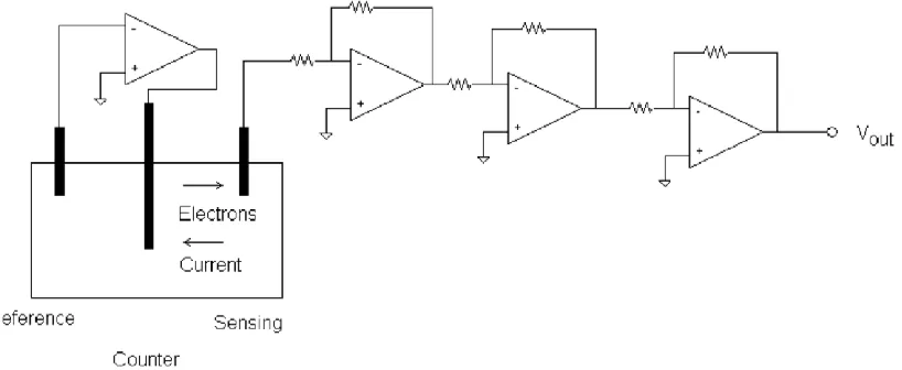
The three terminal 4HS/LM Cititech sensor head (shown in figure 3.1) detected

the hydrogen sulfide. Inside the sensor head the three terminals were attached to a

sensing, counter, and reference electrode suspended in a liquid electrolyte. The

electrolyte was immobilized within the sensor head by a diffusion barrier that allowed

hydrogen sulfide to pass. Externally the three electrodes were attached to a potentiostat

circuit as shown in figure 3.2.

21

The potentiostat works by using a voltage to drive a normally corrosion prone

electrode into immunity and measuring the current required to maintain that immunity.

The hydrogen sulfide causes a reaction to occur at the anode (reference electrode) that

under most circumstances would corrode the anode and release electrons (See equation

3.1) flowing toward the cathode (sensing electrode) where a counter reaction would

occur (see equation 3.2). In a potentiostat the movement of electrons is stopped by an

op amp in an open loop configuration that forces a specified voltage difference between

the anode and the counter electrode. Theoretically, no current passes through the anode

(reference electrode) which prevents the anode from corroding. The op amp draws

current from the solution through a third electrode (counter electrode). This current

causes a voltage difference proportional to the hydrogen sulfide concentration in the

electrolyte between the sensing and the counter electrode. Since the counter electrode is

not an anode prone to corrosion, this signal is stable.

The small voltage difference generated in the potentiostat is measured with a 10

ohm voltage divider and a high gain three stage junction field effect transistor (JFET)

amplifier circuit. This circuit measures hydrogen sulfide up to 100 ppm and the

maximum overload is 500 ppm. This signal is about 0.15 uA/ppm with a sensitivity of

0.1 ppm. In less than five seconds this sensor will react to the presence of hydrogen

sulfide.

Methane Sensor

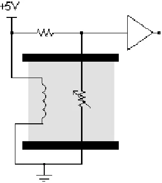
A MQ-5 Hanwei sensor head, as shown in figure 3.3, was used to detect

methane. The resistance of this sensor varied with the log concentration of methane. A

voltage divider converted the resistance into a voltage (see figure 3.4). A voltage

22

loading when the signal went to the data logger. In less than 10 seconds these sensors

can measure from 1-10% methane.

Figure 3.3: Methane Sensor

Figure 3.4: Circuit to Drive Methane Sensor

3.2.2

Volumetric Flow Sensors

The gas sensors used in this experiment were developed to detect hazardous

concentrations of gas. Because both types of sensors were designed for use in the

atmosphere, they rely on the presence of atmospheric oxygen to work. Thus it is

necessary to dilute biogas with air for concentration sensors to work. For safety reasons,

the dilution ratio used in this experiment was less than one part biogas to forty parts air.

One part biogas to ten parts air was avoided because at that ratio the flash point of the

23

Figure 3.5: Volumetric Flow Sensing System

The system shown in figure 3.5 was designed to measure the volumetric flow of

the diluted biogas. This system was designed to handle corrosive biogas and measure

small changes in the diluted flow. Going from left to right at the top of figure 3.5,

24

valve was used to regulate the airflow going into two rigid, smooth walled, two meter

(six foot) fiberglass tubes with a diameter of 2.54 cm (1 in). The tubes had a distance

roughly eleven times the diameter before and three times the diameter after each

measuring point. This was so the flow would to take on the characteristics of a slow,

incompressible Poiseuille flow with a parabolic velocity profile at each of the sampling

points.

The biogas was released into the middle of these tubes between the two

sampling points. One pitot tube was placed at a sampling point before to location the

biogas was injected into the tube and another was placed at a sampling point after the

biogas was injected. The pitot tubes were oriented vertically and pointed into the middle

of the flow. The height of the pitot tube was adjusted until the signal was maximized

from an attached Setra model 264 differential pressure sensor (middle of figure 3.5.)

The deflection of a stainless steel membrane within the sensor was used to measure the

difference in pressure between the two points.

The pressure difference (ΔP) was directly proportional to the volumetric flow

(Q). This relation is evident in the Poiseuille equation (equation 3.3) which relates

pressure change through a tube to dynamic viscosity (µ) of the fluid, the effective length

between the pitot tubes (L), and effective radius of the tube (r) for a laminar flow. This

equation could not be used directly to calibrate the apparatus because of how apparatus

was built. There was a severe constriction of the tube at the location where biogas was

injected. This constriction aided in the mixing of the gasses, but it caused too much of a

pressure drop at that point for the Poiseuille equation to be useful. The Poiseuille

equation is still useful to show that there is a relation between the pressure difference

and the volumetric flow and more importantly that the pressure difference can be used

to measure the volumetric flow.

25

The voltage signal from the pressure sensor was recorded on a data logging circuit. A

specialized circuit (bottom of figure 3.5) was built to measure the pressure sensor voltage

with a sensitivity in the millivolt range and all the electrical noise attenuated. Table 3.1 lists

the features that were needed to attenuate the noise. This table is fully explained in section

C.2 in the Appendix.

Figure 3.6 is the quiescent output of the flow measuring circuit with the ability to

attenuate the normally 20 mV thermal noise to less than 1 mV before sending the signal to

the data logger. As evident in figure 3.6 there was no biasing circuitry built into this

system so the average quiescent voltage is not exactly zero volts.

Table 3.1: Summary of Features of Flow Circuit

Feature Reason Used Issue Addressed

JFET op-amps extreme input impedance flow sensor loading

switching power supply well regulated supply variation in loading

analog and digital supply separation

no power supply

crossover noise from processor

reference point supplied by the software

no reference point

crossover floating ground

shielded sensor cable grounds EM noise electromagnetic signals

twisted pair sensor cable cancels cable inductance crosstalk

solid copper sensor cable low impedance loading effect of cable

100 samples per ten second averaging filter

high frequency filter with no distortion

26

Figure 3.6: The Low Electrical Noise in the Pressure Sensing Circuit

The processor used for data logging was a rabbit 2000 on a wildcat BL2000

motherboard manufactured by Rabbit Semiconductor. The software was programmed in

Dynamic C++ using ANSI C programming conventions. The code to run the device is

given in appendix D. The main purpose of the software was to take measurements from

the three types of sensor circuits tied to the A/D channels, which were the flow circuit

and the two gas sensor circuits. The software also managed the voltage of the reference

point on the flow sensors. The electrical system is shown in figure 3.7.

-0.2154 -0.2152 -0.215 -0.2148 -0.2146 -0.2144 -0.2142 -0.214

0 5 10 15 20 25 30 35 40 45 50

Vo

lts

(V)

27

Figure 3.7: Signal Conditioning Circuitry

3.3

Methods

Each of the sensors were tested for interference from other gasses

(cross-sensitivity). The hydrogen sulfide sensor was tested for cross sensitivity using an

injection of methane gas. The methane sensor was tested using hydrogen sulfide

prepared by reacting sulfur and steel wool with heat and then adding hydrochloric acid.

The sensors were tested for carbon dioxide using a vinegar and baking soda reaction.

The cross sensitivity was negligible in both types of gas sensors.

3.4

Results

The voltage signal from the Setra pressure sensors was converted into a

maximum velocity signal using a calibration curve. The calibration curve was

generated using data recorded by the pressure measurement circuit while measuring a

series of step increases in flow. At each of the flow steps the maximum velocity (or Microprocessor /

Datalogger

CH4 Sensor Conditioning

Circuit

H2S Sensor Conditioning

Circuit

Power Supply

28

the center velocity) of the air leaving the tube was recorded with a Seirra Instruments

610 Flo-meter (air velocity meter) with an Accu-FloTM self-heated platinum

resistance temperature deflector. The signal from the Setra sensors is plotted against

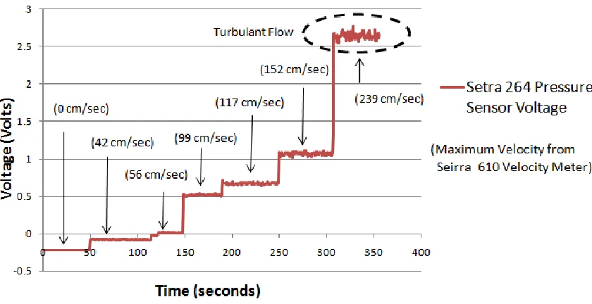
time in figure 3.8 with the maximum velocity measured from the Seirra air velocity

meter recorded at each step.

Figure 3.8: Graph Comparing the Voltage of the Pressure Sensor Circuit to Maximum Velocity Over a Series of Flow Step Increases

Most of the flow measurements were laminar. The effects of turbulence were

evident at 239 cm/sec on both the curve in figure 3.8 and on the Seirra air velocity

meter. For the flows not affected by turbulence (laminar flows) a characteristic equation

relating the maximum velocity to the voltage from the pressure sensors was developed

29

Figure 3.9: The Linear Relationship between the Maximum Velocity and Pressure

Sensor Voltage

The laminar range of maximum velocities measured by the pressure sensors was

from 40 to 160 cm/sec and the resolution was less than 0.1 cm/sec. The resolution was

based on the standard deviation from the mean flow signal.

The maximum air velocity measured in the laminar flow was converted to an

average air velocity by dividing the maximum by two. The laminar flow was verified by

observing turbulence on both the pressure sensors and air velocity meter. The flow was

further verified by cross checking with a WE Anderson prandtl tube and Alnor 560

monometer. (The data for these measurements are in appendix F.) The average velocity

was converted into a volumetric flow rate by multiplying by the cross-sectional area of

the tube.

For the concentration sensors, a similar calibration curve was developed. Before

these sensors would work they had to remain powered for twenty-four hours to reach

chemical equilibrium. The valve on the cylinder with the simulated biogas was opened

releasing a step input of biogas into the airflow within the tubes. This gas deflected the

y = 94.419x + 51.623 R² = 0.997

0 20 40 60 80 100 120 140 160 180

-0.5 0 0.5 1 1.5

30

voltage of the Setra pressure sensors. Figure 3.10 shows such a deflection occurring

between twenty and one hundred seconds.

Figure 3.10: The Signal Given When the Flow Changes from a Steady Flow of Air to a Diluted Flow

The slight change in volumetric flow when the step input of biogas was diluted

in the flow through the tube was measured. Because the initial concentrations of

hydrogen sulfide and methane in the biogas were known, it was possible to calculate the

concentration of the biogas in the diluted flow. The deflection of the voltage in the gas

sensing circuit when a forty five second pulse of biogas was added (see figure 3.11) was

used relate the voltages of the gas sensing circuit to the concentration of the component

gas concentrations in the biogas. This was repeated using different flow rates of the

simulated biogas (see figure 3.12).

70.5 71 71.5 72 72.5 73 73.5

0.0 20.0 40.0 60.0 80.0 100.0 120.0 140.0 160.0 180.0 200.0

Vol

u

m

rti

c

Fl

ow

(c

m

^3/sec)

Time (sec)

Biogas off

31

Figure 3.11: The Voltage Signals from the Gas Sensors when a Forty-Five Second Pulse of Biogas was added to the Diluted Flow

Figure 3.12: The Concentration versus the Flow Sensor Voltages

0 0.2 0.4 0.6 0.8

0.0 100.0 200.0 300.0 400.0 500.0 600.0

voltag

e

(V)

time (sec)

0.0 100.0 200.0 300.0 400.0 500.0 600.0

voltag

e

(V)

time (sec)

0 10 20 30 40 50 60

vo

ltage

(V)

hydrogen sulfide concentration (ppm)

Sensor 1 Sensor 2 2.5 3 3.5 4 4.5

0 1 2 3 4

vo

ltage

(V)

methane concentration (%)

Sensor 1

32

Using a linear regression for the hydrogen sulfide sensor and a normal regression

for the methane sensor it was possible to produce a characteristic equation relating the

voltage signals coming from the gas sensors to the concentrations of the component

gases. (See figure 3.13)

The hydrogen sulfide sensors were rated between 0 and 100 ppm and the

methane sensor was between 0% and 10%. The resolution of the concentration sensors

were limited by the resolution of the flow sensors and the 12-bit analog to digital sensor.

The gas sensors operated between 0 and 5V and had a resolution of 2.44 x 10-4 V.

Figure 3.13: The Concentration Regressed on the Flow Sensor Voltage

y = 0.0436x + 0.1544 R² = 0.9738 y = 0.0379x + 0.0914

R² = 0.9713 0 0.5 1 1.5 2 2.5

0 10 20 30 40 50 60

vo

ltage

(V)

hydrogen sulfide concentration (ppm)

Sensor 1 Sensor 2 Linear (Sensor 1) Linear (Sensor 2)

y = 0.2177ln(x) + 4.0509 R² = 0.8511 y = 0.3886ln(x) + 3.6976

R² = 0.9441 2.5

3 3.5 4 4.5

0.1 1 10

vo

ltage

(V)

Sensor 1 Sensor 2 Log. (Sensor 1) Log. (Sensor 2)

33

3.5

Conclusion

A new inexpensive instrument built from off the shelf components was

developed to measure both the flow and concentration of methane and hydrogen sulfide

in biogas. This system used the properties of a Poiseuille flow to measure the flow of

the gas. A maximum velocity was measured and converted into a volumetric flow. This

system used the electro-chemical properties of liquid and solid-state solutions to

measure the concentration of hydrogen sulfide and methane in the flow.

Using electronic sensors to detect the quality of biogas opens up the possibility

of using on-line monitoring and closed loop control of digesters to improve of biogas

quality. The limitation of the device is the sensors require oxygen to work. Before

biogas can be burned, it must be diluted with oxygen so this system may find a practical

niche in that situation. This instrument is best suited for its primary purpose which is to

34

CHAPTER 4

Testing Biogas Passed Through a Gas-Gas Membrane

System for

Hydrogen Sulfide Removal

4.1

Introduction

Higher fuel costs are driving research into selective gas-gas membranes. Gas-gas

membranes are already being used to improve sour natural gas; so there may be

potential for membranes to improve biogas. Biogas quality can be improved by

separating biogas and removing the acid gases – of which the most detrimental to biogas

quality is hydrogen sulfide (as shown in table 4.1). Most hydrogen sulfide removal

technologies require a high energy phase change, a complex mechanism, or a large

mechanical footprint which is not required by a gas-gas membrane system. One such

gas-gas membrane system was tested for its ability to remove hydrogen sulfide using a

new, experimental sensor system developed specifically for testing hydrogen sulfide

removal.

Table 4.1: Metrics for Biogas Quality Based on the Hydrogen Sulfide Concentration

Concentration of Hydrogen Sulfide Usefulness of biogas

4000 ppm Typical Biogas 600 ppm High Quality Biogas below 100 ppm Safe for Natural Gas lines

below 4 ppm Can be Sold Commercially

Information from Hao, Rice and Stern (2002)

Selective gas-gas membrane research started in 1866 when Graham reported a

rubber polymeric membrane increased the concentration of oxygen in air from 21% to

41%. Based on this work, he proposed the absorption - diffusion - dissolution model for

membrane transport (Ghosal and Freeman, 1994), which is similar to the transport

35

This research is one of the few attempts to study gas-gas membrane technology

as a means to remove hydrogen sulfide from animal manure biogas since a 1988 study

where twelve membranes were tested. None of the membranes were effective for

removing hydrogen sulfide (Kayhanian and Hills, 1988). These membranes were made

of only a single material. The technology has since advanced to include composite

membranes. Composite membranes use different combinations of materials with various

sorption and sieving properties. These materials include: cellulose acetate (Stern

et al., 1998), polyimide (Hao, Rice and Stern, 2002; Quinn and Laciak, 1997; Hillock,

2005; Harasimowicz et al., 2007), polypropylene (Kreulen et al., 1992), polysulfone

(Stern et al., 1998; Harasimowicz et al., 2007), zeolite (Zhu et al., 2005), and

tri-bromodi-phenylopolycarbonate (Harasimowicz et al., 2007).

4.2

Theory

4.2.1

Selectivity Mechanisms

Membranes use two different mechanisms to select one gas over another:

diffusivity and sorption.

A diffusivity difference between two gases means the gas with a smaller

molecular size passes through a porous structure faster than the gas with large molecular

size. The relative size of the molecule can be empirically estimated by measuring

critical volume. A list of critical volumes is given in table 4.2. Diffusivity may be

affected by the shape of a molecule (see figure 4.1). An asymmetric molecule like

hydrogen sulfide can pass rapidly through a membrane by a series of diffusion jumps

36

Figure 4.1: The Molecular Shapes of Component Gases in Biogas

A sorption difference between two gases means one gas will dissolve into

and form again on the other side of a membrane faster than the other. The ability of

a gas to sorb through a membrane is related to critical temperature (the temperature

at the triple point). A gas with a lower critical temperature will sorb quickly

through a membrane because it can condense on the face of the membrane quickly.

The critical temperatures of different gases are given in table 4.2 (Lin

and Freeman, 2005).

Table 4.2: Properties of Component Gases used to Select one Gas Over the Other

Penetrant Critical Volume ( ) Critical Temperature (°K)

H2 65.1 33.24

N2 89.8 126.20

CH4 99.2 191.05

CO2 93.9 304.21

H2S 98.5 373.53

Between hydrogen sulfide and methane, there is not as much difference between

critical volumes as there is between the critical temperatures. Because of the critical

temperature difference it is better to separate biogas using a membrane designed for

sorption. Hydrogen sulfide – which is the unwanted gas – sorbs faster than methane

through a membrane, therefore a membrane separating biogas by sorption has to be in a Hydrogen Sulfide

37

reverse selective configuration. In a reverse selective configuration the hydrogen sulfide

is squeezed out of the biogas through the membrane leaving the methane behind in the

retentate.

In order to sorb, the gases must dissolve into the surface of the membrane. When

acid gases like hydrogen sulfide dissolve into a membrane, the membrane absorbs the

gas and swells up. This swelling is referred to as plasticization (Hillock, 2005).

After plasticization, the concentration of a gas on the surface of the membrane

can be modeled using Henry’s law. (Other isotherms may be used for this step, but Henry’s Law is the simplest and the one most commonly used in literature.) Henry’s

law is given in equation 4.1. CH2S is the concentration of hydrogen sulfide at the surface of the membrane, KHH2S is Henry’s constant for hydrogen sulfide, and pH2S is the partial

pressure of hydrogen sulfide in the biogas.

(4.1)

To quantify separation performance (throughput) of the membrane the model

includes diffusivity. Diffusion is described by Fick’s law which is given in equation 4.2.

In this equation JH2S is diffusion flux of hydrogen sulfide through the membrane, DH2S is the diffusion coefficient for hydrogen sulfide, x is the length or thickness of the

membrane, and ∂C/∂x is the concentration gradient across the membrane.

(4.2)

Integrating diffusion across length of the membrane (equation 4.3) gives the

empirical form of the equation. CHH2S is the concentration of hydrogen sulfide on the

38

sulfide on the low pressure side of the membrane. l is the thickness (length) of the membrane.

(4.3)

Putting dissolution and diffusion steps in series yields equation 4.4 where pHH2S

is the partial pressure of hydrogen sulfide on the high pressure side of the membrane

and pLH2S is the partial pressure of hydrogen sulfide on the low pressure side of the

membrane.

(4.4)

Permeability is defined as the diffusion coefficient times Henry’s constant for a

particular gas crossing the membrane. (Barrer, 1927) (See equation 4.5) Permeability is

defined with a capital

P

(4.5)

Volumetric flow of the gas equals the flux of the gas times the area of the

membrane. Equation 4.6 is for volumetric flow across the membrane with

A

(4.6)

Rearranging the terms in equation 4.6 yields permeability in all measurable

39

(4.7)

The unit for permeability is a barrer. Assuming standard temperature and

pressure conditions a barrer is defined in equation 4.8.

(4.8)

Permeability is generally simplified if the membrane is a asymmetric or

composite membrane such as the one in this experiment. The thickness term (l) is

dropped from equation 4.7 defining a gas permeation unit (GPU) (see equation 4.9).

(4.9)

If the membrane is working properly, different gases will have different

permeabilities. The ratio of permeabilities for two different gases is the membranes

selectivity (

α

(4.10)

One of the challenges in membrane selection is to get a membrane that has both

high permeability (production) for the target gas and high selectivity (efficiency).

4.3

Materials

40

hydrogen sulfide, and retaining methane. It is an asymmetric membrane with the

selective layer composed of a polyamide-polyether block copolymer on top of a macro

porous layer. Polyamide-polyether copolymers are an ideal material because it remains a

rubber at temperatures as low as 0°C and as high as 150°C (Blume and Pinnau, 1990).

Simulated biogas that contained 1000 ppm hydrogen sulfide, 60% methane,

balanced with carbon dioxide was supplied from a pressurized tank through a stainless

steel regulator into custom made membrane holder that resembled the holder used by

Kayhanian and Hills (1988). The membrane holder was made of two 15 x 15 x 0.6 cm (

6” x 6” x 1/4”) steel plates with two couplings welded into each plate. Small c-clamps

clamped the steel plates together at each of the four corners. Two rubber sheets were

made into gaskets for the membrane. An exploded view of the holder assembly with the

membrane is given in figure 4.2.

Figure 4.2: An Exploded View of the Membrane Holder with the Membrane in it

The membrane cell, which held the pressurized gas behind the membrane, was

fastened to the holder and made from a 2.5 x 2.5 x 2.5 cm (1”x1”x1”) T-fitting and a

coupling. Rubber stoppers were inserted into pressurized end of the cell and into the Membrane

41

pipe facing the membrane. A polyethylene tube was threaded from the pressurized

stopper, through the stopper close to the membrane and back through the stopper close

to the membrane. The tube was cut and twisted in a manner that forced the biogas across

the membrane. The volume of the space behind the membrane was reduced as much as

possible to minimize transient effects caused by air being flushed out when it was

pressurized with biogas.

All parts of the membrane cell were made of polyethylene,

polytetrafloroethylene, rubber, stainless steel, or were coated with fiberglass resin to

prevent the absorption or accumulation of hydrogen sulfide.

(a) Low Pressure Side

(b) High Pressure Side

Figure 4.3: Pressurized Chamber Mounted on the Membrane Holder

42

Two types of chemical sensors and the signal conditioning circuitry described in

chapter three were used to detect hydrogen sulfide and methane concentrations. These

sensors were mounted, as shown in figure 4.4, in a way that directed the gas stream directly

into the sensors.

Figure 4.4: Gas Sensors Mounted on the Apparatus

Figure 4.5 is a close-up of the different mechanisms attached to the membrane

holder. On the left side of the figure is the cylinder containing biogas and the regulator.

Under the square plates of the holder is the pressurized chamber shown in figure 4.3. On

the right of the holder is a pin valve used for restricting the release of biogas from the

retentate. The setting of the pin value is determined by the number of turns from its

closed position. Two fiberglass tubes capture and dilute the biogas released from the

permeate and the retentate side of the membrane with air. These tubes are long and rigid

with smooth walls to promote a laminar velocity profile. Inside each fiberglass tube two

pitot tubes are mounted for the purpose of detecting the change in pressure as the gas

moved down the tubes. Air is driven through the fiberglass tubes using a blower from a

shop vacuum cleaner. The air flow is controlled by adjusting two ball valves on a

43

fiberglass tubes to both hold the gas sensors and deflect wind. Pieces of surveyor’s tape

are draped over the cups as a safety feature to verify the air was flowing.

44

Figure 4.6: Complete Apparatus

4.4

Methods

There were conflicts between the quality of the results and safety of the

experiment. A dilution ratio between forty and one hundred parts air to biogas had to be

used to prevent the temperature of the air/biogas mixture’s flash point from dropping

low enough to explode. Because of the dilution, specialized conditioning circuitry was

designed and special data processing methods used for high precision measurement of

the volumetric flows.

Because hydrogen sulfide is toxic and the apparatus was too large to fit under a

hood, the experiment had to be performed outdoors and attended constantly.

Temperature was impossible to control, so thermal drift had to be compensated for in

very small voltage signals. This was done by subtracting the linear time dependent trend

in the quiescent flow voltage signal observed before the biogas was pressurized from the

entire signal including the portion after the biogas was pressurized.

The measurement system for the apparatus was fully automated. When the