Nonparametric models for longitudinal data using Bernstein polynomial sieve

Nonparametric Models for Longitudinal Data Using

Bernstein Polynomial Sieve

Liwei Wang and Sujit K. Ghosh

Department of Statistics, North Carolina State University

Abstract

We develop a new nonparametric approach to the analysis of irregularly observed longitudinal data using a sieve of Bernstein polynomials within a Gaussian process framework. The proposed methodology has a number of novel features: (i) both the mean function and the covariance function can be estimated simultaneously under a set of mild regularity conditions; (ii) the derivative of the response process can be ana-lyzed without additional modeling assumptions; (iii) shape constraint of the mean and covariance functions (e.g. nonnegativity, monotonicity and convexity) can be handled in a straightforward way; and (iv) theLp approximation of the Gaussian process using the Bernstein polynomial sieve is established rigorously under mild regularities condi-tions. Further, in order to choose the appropriate order of the Bernstein sieve, a new Bayesian model selection criterion is proposed based on a predictive cross-validation criterion. Superior performance of the proposed nonparametric model and model se-lection criterion is demonstrated using both synthetic and real data examples.

Key Words: Bernstein polynomial sieve, Gaussian process, longitudinal data, MCMC

methods, mixed effects model.

1

Introduction

In a wide variety of disciplines such as agriculture, biology, business, epidemiology, medicine,

and social science, data are collected repeatedly at a sequence of time points on randomly

selected subjects. One typical example involves observations from the sample path of a

growth curve (see Figure 3), where height/weight of a subject is measured repeatedly over

time. In addition, some other related predictors such as gender and treatment group are also

recorded at the baseline. Longitudinal models target at modeling the relationship between

the response curves and predictors. Meanwhile, the mean of response curves is sometimes

required to satisfy certain shape constraints such as non-negativity, monotonicity and

con-vexity. For example, a growth curve must be nondecreasing, and recorded height/weight

must be positive. In order to obtain a realistic estimate of the response curve, the natural

shape constraints should also be considered and preserved for any finite sample estimator.

Longitudinal study involves temporal order of exposure and outcome, which requires the

modelling of the auto-correlation function within the subject. Common practice assumes

that the response is the additive effects of three parts: the fixed effects, which capture the

underlying trend; the random effects, which capture the heterogeneity across subjects; and

the noise part, which captures the observational or measurement errors. Linear mixed

ef-fects model (LMM; Laird and Ware 1982) is widely used such that both the fixed efef-fects

and the random effects are linear functions of some predictors, and the the vector of the

random effects follows a multivariate Gaussian distribution. The noises are also assumed

independently of the random effects to follow some Gaussian distribution with mean 0.

Many standard software packages are available (e.g. PROC MIXED in SAS, lme in R,

etc.) which allows the estimation of the parameters using maximum likelihood (ML;

Robin-son 1991), restricted maximum likelihood (REML; PatterRobin-son and ThompRobin-son 1971; Harville

1977), or expectation-maximization (EM) algorithm (Lindstrom and Bates 1988). But LMM

is based on the linearity assumption that relates responses to predictors and also the

covari-ance matrix are often chosen parametrically assuming regularly spaced sequence of time

points. When the relationship between the response and predictors are nonlinear and data

correlation structure.

Nonlinear mixed effects models (NLMMs) are proposed to handle the complex

relation-ship between response and predictors. Davidian and Giltinan (1995), Davidian and Giltinan

(2003), and Serroyen et al. (2009) provided comprehensive reviews on NLMM with various

applications in practice. When we can identify the form of nonlinear relationship from the

mechanistic theory, the parametric NLMM is employed. Some typical applications include

the pharmacokinetics and pharmacodynamic modeling (Davidian and Giltinan 1995,

Ch-pater 5), HIV dynamics modelling (Han and Chaloner 2004), and prostate specific antigen

modeling (Morrell et al. 1995). Moreover, classical NLMM can be implemented directly in

some popular statistical software, such as PROC NLMIXED in SAS and nlme in R. However,

the assumption that the functional form of the nonlinear relationship is known may often

turn out to be restrictive. Misspecified nonlinear relationship is likely to cause improper use

of NLMM. Ke and Wang (2001) proposed a semiparameteric NLMM and applied their model

to AIDS data, where only the mean function is modelled nonparametrically. A

nonparamet-ric NLMM was proposed by Lindstrom (1995), which replaced the nonlinear function with

a free-note spline shape function. But the resulting covariance structure fitted in this way is

not easy to interpret. In general, although NLMM provides a greater flexibility in capturing

the possible relationships between the responses and predictors, the model is still based on

an assumed nonlinear functional form which may only be a crude approximation to the true

relation between the response and predictors. Moreover, in practice the correlation function

is often modelled parametrically.

Assuming every response curve is a realization of a Gaussian process at certain time

points, functional principal component analysis (FPCA) is an alternative way to tackle such

longitudinal data problem owing to the Karhunen-Lo`eve (K-L) expansion of a Gaussian

with linear combination of eigenfunctions. Di et al. (2009) presented method of moments

and smoothing techniques to obtain a smooth estimator to the covariance function and its

corresponding eigenfunctions. Staicu et al. (2010) suggested the use of a restricted likelihood

ratio test which is a step-wise testing for zero variance components in order to select the

number of eigenfunctions. Crainiceanu and Goldsmith (2010) gave an example applying

the functional principal component analysis on the sleep EEG data. However, to implement

FPCA, in practice one often use empirical estimates of eigenfunctions in the first place which

may cause problem when sample size is not large and when observations are very sparse or

missing or censored. Also in Crainiceanu and Goldsmith (2010)’s example, they used the

sample mean at every time point to estimate the mean function, which is too rough and may

not satisfy a required shape constraints. One of the most common limitations of the FPCA is

that these methods are primarily based on two stages of estimations: (i)the eigenfunctions are

estimated based on estimated residuals and then (ii) these estimated functions are plugged-in

to estimate the mean function or to predict the future observations assuming the estimated

functions are “known” functions. These plugged-in estimated functions often lead to the

underestimation of the overall uncertainty of the predictive process.

In the present paper, we propose a class of linear mixed effects models using Bernstein

polynomial sieve to overcome some of the limitations mentioned above. With our proposed

model, under a set of mild regularity conditions on the Gaussian process, we first establish the

uniform approximation of an arbitrary Gaussian process by a sieve of Bernstein polynomials.

Convergence properties of our proposed model are established in terms of L2 and more

generally for Lp norms under some mild regularity conditions. Additionally, we can easily

incorporate shape restrictions of the mean curves by utilizing the attractive properties of

Bernstein polynomials which allows us to model various popular shape constraints such as

method for finite sample, we still need to “choose” the order of the Bernstein sieve. A

new Bayesian model selection criterion based on predictive divergence is proposed. Several

simulation studies are presented to illustrate its superior performance compared to some

popular Bayesian model selection criteria.

The paper is organized as follows. Section 2 presents the class of linear mixed models

using Bernstein polynomial sieve to approximate the longitudinal model within a Gaussian

process framework. Meanwhile, a new model selection criterion which we call the Bayesian

predictive divergence criterion (BPDC) is proposed and computation details are described.

In Section 3, the approximation properties of the proposed model are discussed. The

cor-responding proofs are provided in the (web) Appendix. Section 4 presents two simulation

studies. One is to examine the performance of BPDC by comparing with a few of the popular

Bayesian model selection criteria. The other is to examine the accuracy of the approximation

model using Bernstein polynomials to a Gaussian process with nonlinear mean and complex

covariance functions. In Section 5, our proposed model and criterion are illustrated on the

Berkeley growth data. Finally, a discussion of the proposed methodology and future research

work are presented in Section 6.

2

Gaussian Processes Approximation with Bernstein

Polynomials

Let Yi(t) denote the measured response obtained at time t ∈ [0, T] for subject i. Suppose

we observe Yi(t) at selected set of time points ti,1 < ti,2 < . . . < ti,Ji where Ji ≥ 2 for

i = 1, . . . , I. Denote yi,j = Yi(ti,j) for j = 1, . . . , Ji and i = 1, . . . , I. To begin with, for

simplicity we consider a simple longitudinal model with t as the only predictor. Additional

predictors can be easily incorporated in the model. Let GP(µ(·), K(·,·)) denote a Gaussian

the underlying model for the simple longitudinal study is given by,

Yi(t) =Xi(t) +i(t), i= 1, . . . , I, (1)

where Xi(·) iid

∼GP(µ(·), K(·,·)), and i(·) iid

∼GP(0, σ2

I(·,·)) where I(t, t

0_{) = 1 if t=t}0 _{and 0}

otherwise. In practice, we often do not have any specific knowledge to specify the functional

forms, but some shape properties of µ(·) may be known (e.g. growth curves are necessarily

non-decreasing, etc.). To fit Model (1) without loosing much accuracy, we propose a class

of linear mixed effects models using a sieve of Bernstein polynomials as an approximation,

where Bernstein polynomial is employed due to its optimal property in retaining the shape

information (Carnicer and Pena 1993). To start with, we give a brief introduction to some

attractive properties of Bernstein polynomials.

2.1

Shape Restricted Bernstein Polynomials

The Bernstein polynomials (BP) were introduced by Sergei Natanovich Bernstein in 1912,

and since then this class of polynomials has become one of the most popular classes of

polynomials in numerical analysis. Lorentz (1953) is a complete handbook on Bernstein

polynomials, including complete proofs of many interesting theorems related to Bernstein

polynomial and its generalizations.

The Bernstein basis polynomials on [0,1] of degree m−1 is defined as

bk,m(t) =

m−1

k−1

tk−1(1−t)m−k, k = 1, . . . , m, t∈[0,1], m = 2,3, . . . . (2)

The Bernstein polynomial sieve (BPS) of order m−1 is defined as any linear combination

of Bernstein basis polynomials,

Bm(t) = m X

k=1

ak,mbk,m(t), t ∈[0,1], (3)

where ak,m can be any real number. Notice that BPS includes iterates of BP’s which enjoy

and infinitely many differentiable on [0,1]. One of the nice properties of BPS is that the

derivatives of a BPS is still a BPS of a lower degree. In fact, it is well known that

B_m0 (t) = (m−1)

m−1 X

k=1

(ak+1,m−ak,m)bk,m−1(t), (4)

and more generally, the l−th order derivative is still a BP and is given by

B_m(l)(t) =l!

m−1

l

m−l X

k=1

∇(l)ak,mbk,m−l(t), (5)

where ∇(l)_a

k,m = ∇(l−1)ak+1,m − ∇(l−1)ak,m for l = 1,2, . . ., and ∇(0)ak,m = ak,m. From

above, it follows that linear restrictions on the coefficients ak,m’s induce restrictions on the

derivatives ofBm(t) fort ∈[0,1]. For example, if a1,m ≤a2,m ≤. . .≤am,m, then Bm0 (t)≥0

for t ∈ [0,1]. Thus shape constraints like nonnegativity, monotonicity, and convexities can

be easily imposed by using finite dimensional linear inequality constraints on the coefficients.

Gal (2008), Chapter 1, provided complete proofs to many shape-preserving properties and

more interesting properties. Wang and Ghosh (2012) elaborated some of the interesting

results on monotone function, convex/concave function, and monotonous convex function,

and established the strong consistency property of Bernstein sieve using constrained least

square estimation of the mean function only.

Meanwhile, the convergence properties of Bernstein polynomials to continuous functions

have been thoroughly studied. Lorentz (1953), Chapter 1, described the Bernstein

Weier-strass approximation theorem which provides the convergence properties of Bernstein

polyno-mials inL∞norm. Hoeffding (1971) discussed theL1 norm approximation error for Bernstein

polynomials. Jones (1976) proved several theorems for the approximation error for Bernstein

polynomials inL2 norm. More recently, Khan (1985) generalized the convergence of BPS to

Lp norms under mild regularity condtions. All these theorems assist us to understand the

2.2

A Class of Linear Mixed Effects Models with Bernstein

Poly-nomials

Suppose both mean function and covariance function are continuous and satisfy some mild

regularity conditions (as stated in Theorems 1 and 2 in Section 2.3), we claim that the Model

(1) can be approximated by the following class of linear mixed effects models using a sieve

of Bernstein polynomials (as m→ ∞),

Yi(t) = m X

k=1

bk,m(t)βi,k+i(t), i= 1, . . . , I, (6)

where βi = (βi,1, . . . , βi,m)T, βi iid

∼ N(β0, D) and i(t) iid

∼ N(0, σ2). Also, we may assume

i(t) ind

∼ N(0, σ2

i) to represent heterogenous errors. With data {yi,j} observed, we can use

Bayesian methods to fit the model for each m,

yi,j = m X

k=1

bk,m(ti,j)βi,k +i,j, i= 1, . . . , I, (7)

with some proper prior assigned to θ = (β0, D, σ2). Finally, the order m of the Bernstein

sieve is chosen using a predictive criterion.

It is easy to see that with Model (6), we have approximated true Xi(t) GP with the

Gaussian process

GP

m X

k=1

bkm(t)β0,k, m X

k=1 m X

h=1

bk,m(t)bh,m(s)Dk,h !

. (8)

The details of the convergence result is presented in Section 3. Ifµ(·) andK(·,·) are assumed

differentiable, and as differentiation is a linear operation (Solak et al. 2003), the derivative

of a Gaussian process X(·)∼ GP(µ(·), K(·,·)) is still a Gaussian process such that X0(·)∼

GP(µ∗(·), K∗(·,·)), where µ∗(t) = µ0(t) and K∗(t, s) = ∂2_∂t∂sK(t,s). So we can also explore the

the derivative of the Gaussian process X_i0(t) in Model (1). Such a derivative process is of

much practical interest when estimating the rate of change of the growth as we illustrated in

et al. 2013). With Equation (5), it can be shown that X_i0(t) is approximated with

GP (m−1)

m−1 X

k=1

bk,m−1(t)(β0,k+1−β0,k), (9)

(m−1)2

m−1 X

k=1 m−1 X

h=1

bk,m−1(t)bh,m−1(s)(Dk+1,h+1−2Dk+1,h+Dk,h) !

.

This follows by another interesting property of BPs which states that the derivatives of the

function are uniformly approximated by the derivatives of the corresponding BPs (Lorentz

1953, Page 13).

LetJ be the number of unique time points in the data set. To avoid collinearity issue with

large degree polynomials, m should always be chosen less than J in Model (6). Tenbusch

(1997) suggested a more strict upper bound for the choice of m in nonparametric regression

with Bernstein polynomials such that m ≤[J3/4_{]. With m = 1, we can only approximate a}

degenerated Gaussian process. Hence, we also require mto be greater than 1. So in practice

the value of m is chosen from set{2, . . . ,[J3/4]} using a predictive divergence criterion that

we describe in the next subsection.

2.3

Bayesian Model Selection using Predictive Divergence

In this subsection, we propose a new Bayesian model selection criterion based on predictive

divergence for the purpose of choosing the tuning parameter m. However, the proposed

criterion is not restricted to the choice of Bernstein sieve model and it can be applied for

general model selection purpose among many competing models. The new cross-validation

model selection criterion, Bayesian predictive divergence criterion (BPDC) is motivated by

Davies et al. (2005) and Geisser and Eddy (1979). We generalize the predictive divergence

defined in Davies et al. (2005) to Bayesian inferential frame work. Suppose the candidate

Bayesian model is y ∼ f(·|θ) with a prior distribution θ ∼ π(θ). We define Bayeisan

with respect to the posterior distribution of θ depending on the leave-one-out data y−i, say

dB_i (y, f) =

Z

−2 logf(yi|θ)p(θ|y−i)dθ, (10)

wherep(θ|y−i) =f(y−i|θ)p(θ)/ R

f(y−i|θ)p(θ)dθ denotes the posterior distribution ofθ given

the datay−i = (y1, . . . , yi−1, yi+1, . . . , yI). The total Bayeisan predictive discrepancy over all

subjects is then defined as

dBP DC(y, f) = I X

i=1

dB_i (y, f). (11)

Taking expectation of dBP DC(y, f) with respect to the true model, we get

∆BP DC(f) = Ey[dBP DC(y, f)], (12)

= Ey[ I X

i=1 Z

−2 logf(yi|θ)p(θ|y−i)dθ]. (13)

Our target is to find an unbiased estimator to ∆BP DC(f). Note that in Equation (13), the

term inside expectation is a function of y. Thus, the term inside is an unbiased estimate of

∆BP DC(f), and we can then define the Bayesian predictive divergence criterion (BPDC) as

BPDC =

I X

i=1 Z

−2 logf(yi|θ)p(θ|y−i)dθ, (14)

=

I X

i=1

−2Eθ[logf(yi|θ)|y−i].

With simple models, we can compute R logf(yi|θ)p(θ|y−i)dθ directly for each i. But

for most of complex Bayesian models with high dimensional θ, it is often not possible to

integrate out θ. In this situation, without losing much accuracy, ideally we can use Monte

Carlo integration to calculate Eθ[logfi(yi|θ)|y−i] by generating samples θ (l)

i ∼ p(θ|y−i) for

l = 1, . . . , L. So one option for computing BPDC in this case is to generate θ(l)_i by MCMC

simulation with data that excludes the ith subject and repeat the procedure for allIsubjects.

This means that we have to run the MCMC simulation I times to get the value of BPDC,

Importance sampling (IS) provides a solution to this computation problem. Gelfand and

Dey (1994), Peruggia (1997), and Vehtari and Lampinen (2002) advocated the use of IS in

computing the expectation with respect to the case-deletion posterior.

Suppose we want to compute the expectationEpi[g(θ)] = R

g(θ)pi(θ)dθwith respective to

the density pi(θ) fori = 1, . . . , I (e.g. pi(θ) =p(θ|y−i), etc.). Instead of generating samples

frompi(θ) and repeat the procedureI times, we can obtain samples from a candidate density

p(θ) and use the identity Epi[g(θ)] = R

pi(θ)g(θ)dθ = R pi(θ)

p(θ)g(θ)p(θ)dθ =Ep[ pi(θ)

p(θ)g(θ)]. Now

ifp(θ) = q(θ)/C andpi(θ) =qi(θ)/Ci are known only by their kernel functionsq(θ) andqi(θ)

respectively, then Epi[g(θ)] can be estimated consistently (as L→ ∞) by

¯ gL =

L X

l=1

g(θ(l)) ¯wl(pi, p),

whereθ(l) iid_{∼p(θ), ¯w}

l(pi, p) =wl(pi, p)/ PL

h=1wh(pi, p), andwl(pi, p) = qi(θ(l))/q(θ(l))

(Perug-gia 1997). The strong law of large number for Markov chains always implies the consistency

of the estimator, but its performance depends critically on the variance of the IS weight

wl(pi, p). For a standard Bayesian linear regression model, Peruggia (1997) proved necessary

and sufficient conditions for finite variance of IS weights.

As the above discussion attests, we can apply IS method to compute BPDC. Suppose we

are given a Bayesian model whereπ(θ) denotes the prior density function of the parameterθ,

a data set y= (y1, . . . , yI) where yi’s are mutually independent vectors given θ, and MCMC

samples θ(l), l = 1, . . . , L, based on the full data y, i.e. θ(l) ∼ p(θ|y). Letting p(θ) =p(θ|y),

pi(θ) = p(θ|y−i),C =m(y), and Ci =m(y−i), we have wl(pi, p) = 1/f(yi|θ(l)), and hence

¯

wl(pi, p) =

1/f(yi|θ(l)) PL

h=11/f(yi|θ(h))

=

L X

h=1

f(yi|θ(l))

f(yi|θ(h)) !−1

Finally, using the above defined IS we can approximate BPDC by

BPDCa = −2

I X

i=1 L X

l=1

logf(yi|θ(l)) ¯wl(pi, p), (15)

= −2

I X

i=1 L X

l=1

logf(yi|θ(l)) L X

h=1

f(yi|θ(l))

f(yi|θ(h)) !−1

.

We use the above approximation to select the sieve order m of our proposed model.

3

Convergence Properties

In this section, we present convergence properties of the finite dimensional approximation

of the GP(µ(·), K(·,·)) by a class of random BPS of the form Pm

k=1bkm(t)βkm, whereβm =

(β1m, . . . , βmm)T ∼N(µm, Dm) as m → ∞.

Theorem 1. Consider a Gaussian processX(t)defined on[0,1]with continuous mean

func-tion µ(t) and continuous nonnegative definite covariance function K(t, s). Suppose λi’s and

ei(·)’s are eigenvalues and eigenfunctions of K, where the first derivatives of the

eigenfunc-tions exist and are continuous. Also assume that

∞

X

i=1

λi Z 1

0

t(1−t)|e0_i(t)|2_{dt <∞}

Then, there exists Xm(t) = BmT(t)βm where Bm(t) = (b1m(t), . . . , bmm(t))T, bkm(t) =

m−1 k−1

tk−1(1−t)m−k, and βm ∼N(µm, Dm) for some µm and Dm, such that

lim

m→∞EkX−Xmk

2

2 = lim_m→∞E Z 1

0

|X(t)−Xm(t)|2dt = 0,

i.e., the sequence of stochastic processes {Xm(t) :t∈[0,1], m= 1,2, . . .} converges in mean

square to the stochastic process {X(t) :t∈[0,1]}.

If we make further assumptions on eigenvalues and eigenfunctions of the covariance

Theorem 2. Let 1 ≤ p < ∞. Consider a Gaussian process X(t) defined on [0,1] with

continuous mean functionµ(t)and continuous nonnegative definite functionK(t, s). Suppose

λi’s and ei(·)’s are eigenvalues and eigenfunctions of K, and continuous derivatives e0i(t)

exists for all i’s. Assume that

(i) P∞ i=1

√

λi{Vp(ei)}1/p<∞, where Vp(ei) = R1

0 t

p/2_(1−t)p/2_|e0

i(t)|pdt, and

(ii) P∞ i=1

√

λikeikp <∞, where keikp ={ R1

0 |ei(t)|

p_dt}1/p_.

Then, there existsXm(t) = BmT(t)βm whereBm(t) = (b1m(t), . . . , bmm(t))T,bkm(t) = m_k−−₁1

tk−1₍₁₋

t)m−k, and βm ∼N(µm, Dm) for some µm and Dm, such that

lim

m→∞EkX−Xmkp = limm→∞E{

Z 1

0

|X(t)−Xm(t)|pdt}1/p= 0, (16)

i.e., the sequence of stochastic processes {Xm(t) : t ∈ [0,1], m = 1,2, . . .} converges in Lp

norm to the stochastic process {X(t) :t∈[0,1]}.

Remark: (1) If λi’s have finitely many non-zero values, condition (i) and (ii) are trivially

satisfied. (2) When p= 2, condition (ii) can be simplified to P∞ i=1

√

λi <∞sincekeik2 = 1.

Ritter et al. (1995) showed that λi ∼ i−2r−2 asymptotically (as i → ∞) if the covariance

function satisfies the Sacks-Ylvisaker condition of order r ≥1. Then, condition (ii) is very

likely to be satisfied when Sacks-Ylvisaker condition meets.

Consider the popular squared exponential covariance function defined on [0,1] such that

K(t, s) = exp{−(Φ

−1_(t)−Φ−1_(s))2

2 }, t, s ∈[0,1], (17)

where Φ−1_{(·) is the quantile function of a standard normal distribution. Fasshauer and}

McCourt (2012) showed that the eigenvalues and the orthonormal eigenfunctions are λi =

3−√5

2

i+1/2

andei(t) =φi(Φ−1(t)), fori= 0,1, . . ., whereφi(t) =γiexp

−

√

5−1 4 t

2_H i(

1 4

q 5 4t),

γi = p

51/4_/(2i_{i!), and H}

i(x) = (−1)iexp(t2)d i

dti exp(−t2) (Hermite polynomial). For p = 1,

q 3−√5

2 < 1 and keik1 ≤ 1. Thus, with Theorem 2, we can show that there always exists a

Bernstein polynomial sieve converges to a Gaussian process with continuous mean function

and square exponential covariance function in L1 norm.

Theorem 1 demonstrates that we can always find a sequence of models based on Bernstein

polynomials that converge to the Gaussian process under some mild regularity conditions in

L2 norm. Since convergence inL2 norm implies convergence in probability and convergence

in distribution, this theorem naturally holds for the cases of convergence in probability and

distribution of Bernstein polynomials approximation to Gaussian processes. Theorem 2

demonstrates an even stronger consistency of our Bernstein polynomial sieve to Gaussian

processes satisfying certain regularity conditions in terms ofLpnorm. Moreover, in the proof

of Theorem 1 and 2, we have explicitly constructed the Bernstein polynomials estimator

where µm and Dm preserve the shape of µ(·) and K(·,·).

Suppose a Gaussian process X(u) is defined on some support setD⊆_Rother than [0,1],

with mean functionµ(u) andK(u1, u2). We can then find a proper invertible transformation

functiont=g(u) which mapsDto [0,1]. Since a Gaussian process is determined by mean and

kernel functions, X(t) with mean functionµ(g−1_{(t)) and kernel functionK(g}−1_(t

1), g−1(t2))

is the equivalent Gaussian process defined on [0,1]. Then under regularity conditions on the

new mean and kernel functions, µ◦g−1 _andK◦g−1_{, we can apply Theorem 1 and 2. In this}

way, Theorem 1 and 2 are naturally extended to Gaussian processes with support sets other

than [0,1].

Our theorems can also be generalized to any other polynomials, since there is a one-to-one

mapping between Bernstein basis polynomials of degreem−1 and power basis polynomials

of degreem−1. So, instead of Bernstein polynomials, we can use other polynomials such as

linear combination of power basis, Hermite polynomials, Laguerre polynomials and Jacobi

listed in Theorem 1 and 2. Moreover, results of Khan (1985) can be used to generalize our

results to many other operators (e.g. Feller operator).

4

Simulation Studies

In this section, various simulated data scenarios are used to compare the performance of our

proposed model selection criterion, BPDC, with two popular Bayesian model selection

crite-ria, Deviance information criterion (DIC; Spiegelhalter et al. 2002) and log pseudo marginal

likelihood (LPML; Geisser and Eddy 1979). Also, a simulation study is conducted to show

the approximation to a Gaussian process with nonlinear mean and covariance functions using

a sieve of Bernstein polynomials.

4.1

Comparison of Bayesian Model Selection Criteria

DIC is frequently used for model selection and the computation is easy by reusing the output

from Markov chain Monte Carlo (MCMC) samples obtained from the posterior distribution.

Most statistical softwares provide value of DIC by default such as WinBUGS/OpenBUGS

and SAS. DIC can have different definitions if parameters of interests are different. We

considered two types of DIC’s in our simulation study, conditional DIC and marginal DIC

(page 282, Lesaffre and Lawson 2012). The leave-one-out cross-validation based criterion,

LPML, is also developed in the frame work of Bayesian analysis, and can be approximately

well by using with MCMC samples along with importance sampling. In our simulation study,

we compared the performance of BPDC with conditional DIC, marginal DIC and LPML. In

accordance with DIC and BPDC, we define LPML = −2PI

i=1logf(y|y−i), where f(yi|y−i)

denotes the posterior predictive density of yi giveny−i.

Data were generated from Model (6). Time points (ti,1, . . . , ti,J) were determined as an

following settings were included in the study. Case 1 is the simplest scenario where the

number of observations for each subject is comparably large and random error variance is

small. The number of observations for each subject is reduced from 30 to 10 in Case 2, while

the random error variance is increased from 0.01 to 0.25. In Case 3, heterogeneous random

errors are considered.

• Case 1: m=4, I=50, J = 30, σ2_i = 0.01 for all i’s, β0 = (1,0.5,0.8,−0.7)T, and D =

0.01I4;

• Case 2: m=3, I=50,J = 10, σ2_i = 0.25 for alli’s, and

β0 = (1,−0.7,2)T,

D =



 

1 0 0.2

0 0.7 0

0.2 0 1.2



 ;

• Case 3: m=3, I=50, J = 10, σ_i2 iid∼IG(5,1), a distribution with mean 0.25, β0 and D

are set the same as in Case 2.

We computed model selection criteria for models with m ranging from 2 up to [J3/4_].

To fit Bayesian models, WinBUGS was used to perform the MCMC methods, where the

first 3000 samples were dropped as burn-in samples and remaining 3000 samples were used

for posterior inference. Table 1 summarizes the percentage of times a model with a given

m∈ {2, . . . ,[J3/4]} is selected based on different criteria. For instance, in Case 1, the (true)

model with m = 4 was selected 96% by BPDC and models with m ≤ 3 and m ≥ 6 were

never selected. It clearly shows that BPDC and LPML always select the correct model

with the highest percentage. On the contrary in Case 3, DIC’s selects the most complex

model (largest m) most of the times. This clearly indicates that DIC’s potentially lead to

selecting over-fitted models in this scenario. Moreover, BPDC outperforms LPML in terms

random error term is large or small, homogeneous or heterogeneous. In particular, for Case

1 where we have many observations for every subject, BPDC selects the correct model with a

proportion as high as 96% which is 12.5% more than the second best one. Moreover, BPDC

selects the incorrect model 9% of the times while the LPML, marginal DIC and conditional

DIC selects incorrect models 17.5%, 16.5%, and 36%, respectively for the Case 1 scenario.

Similar conclusions can also be drawn for Case 2 and 3. This also demonstrates the superior

performance of BPDC compared to DIC’s and LPML.

4.2

Empirical Approximation of Nonlinear Gaussian Processes

with Bernstein Polynomials

In this subsection, by using BPDC as our model selection criterion, we carried out a

simu-lation study to explore the approximation of a Gaussian process with nonlinear mean and

covariance functions using the proposed BPS.

Suppose the true model is Model (1) with σ2

= 0.01. Following the real data example

presented by Wu and Ding (1999), we chose mean function to be

µ(t) = 0.001{exp(12.142−6.188t) + exp(7.624 + 0.488t)}, t ∈[0,1],

and the true covariance function to be the squared exponential covariance function defined

in (17).

We generated 200 data sets, where each data set contains 50 subjects with 10 observations

for each subject. Time points are determined as an arithmetic sequence of length 10 between

0.02 and 0.98 for all subjects. We fit Model (6) for every trial with tuning parameter m

ranging between 2 and 9, and selected the model with the lowest BPDC. WinBUGS was

used to perform the MCMC methods, and the final 3000 out of 6000 MCMC samples were

kept for inference.

mean function and covariance function defined as following:

IBias(ˆµ) =

Z 1

0

{µ(t)−µˆ(t)}dt=

Z 1

0

µ(t)dt−

Z 1

0

ˆ µ(t)dt,

IBias( ˆK) =

Z 1

0 Z 1

0

{K(t, s)−Kˆ(t, s)}dtds=

Z 1

0 Z 1

0

K(t, s)dtds−

Z 1

0 Z 1

0

ˆ

K(t, s)dtds,

where ˆµ(t) = Pm

k=1βˆkmbkm(t), ˆK(t, s) = Pm

k1=1

Pm k2=1

ˆ

Dk1k2bk1m(t)bk2m(s), and ˆβkm’s and

ˆ

Dk1k2’s are posterior means of model parameters. To calculate IBias(ˆµ) and IBias( ˆK), we

just need to compute R1

0 µˆ(t)dt and R1

0 R1

0 Kˆ(t, s)dtds since R1

0 µ(t)dt and R1

0 R1

0 K(t, s)dtds

are fixed once the true mean function and covariance function are determined. With the

formula of derivatives of a Bernstein polynomial, we can compute the integration of a

Bern-stein polynomial quickly. For our case R1

0 µˆ(t)dt = Pm

k=1βˆkm/m and R1

0 R1

0 Kˆ(t, s)dtds = Pm

k1=1

Pm k2=1

ˆ

Dk1k2/m

2_{. The integration of the true mean and covariance function can be}

obtained numerically using R, and we have

IBias(ˆµ) = 31.902−

m X

k=1

ˆ βkm/m,

IBias( ˆK) = 0.577−

m X

k1=1

m X

k2=1

ˆ

Dk1k2/m

2

.

Table 2 presents the Monte Carlo means and Monte Carlo standard errors of these integrated

biases. The mean integrated bias computed based on 200 trials for the mean function and

covariance function, both of which are very close to 0. We also calculated the p-value based

on a one-sample t test for testing whether the integrated bias is significantly different from 0.

For both mean function and the covariance function, the p-values are larger than 0.1, which

demonstrates that there is no significant difference between the true Gaussian process and

the approximated Gaussian process using Bernstein polynomials in terms of integrated bias

at significance level of 0.1. In Figure 2, the true mean function, the estimated mean function,

and the 95% pointwise credible interval are overlaid. Though we used different line color

at every evaluation point the true mean function is always lying between the 95% upper

bound and lower bound. This demonstrates that our Bernstein polynomial approximation

also works very well in terms of pointwise fit.

5

Berkeley Growth Data Analysis

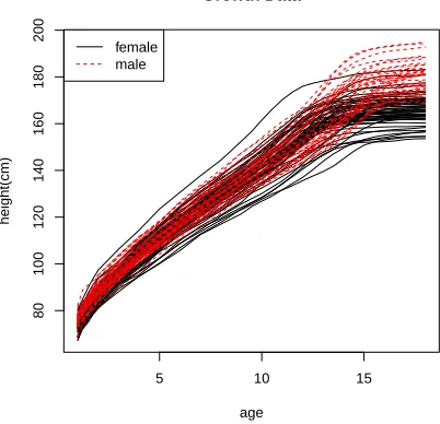
An interesting data set is the Berkeley growth data which monitor the growth of children

from age 1 to age 18. In this study, the heights of 39 males and 54 females were collected at

irregularly spaced time points. It is accessible on public domain with data name “growth”

in package “fda” in R.

Figure 3 shows the growth curves (heights) of the two groups, female and male. Our

goal is to find if there is a significant difference between the growth of females and males in

their youth. In this study, both growth curves and growth rates are of interest. In addition,

we need to consider the nondecreasing constraint in the mean function since human beings

cannot grow shorter during their youth. To model the monotone mean function, we fit the

following model for female and male respectively.

yi,j = m X

k=1

bk,m(ti,j)βi,k+σii,j, (18)

βi iid

∼ N(β0, D),

i,j iid

∼ N(0,1),

with priors

α0 ∼ LogN ormal(0,100I),

D0 ∼ InvW ishart(100I, m+ 2),

σ2_i iid∼ InvGamma(0.01,0.01),

where βi = (βi,1, βi,2, . . . , βi,m)T,β0 = (β0,1, β0,2, . . . , β0,m)T, α0 = (α0,1, α0,2, . . . , α0,m)T,

was used to convert age ∈ [1,18] to t ∈ [0.05,0.9] ⊆ [0,1]. Model selection criteria BPDC

were computed for m = 2, . . . ,14, shown in Figure 4. It is clear that BPDC reach its

min-imum at m=7 for the female group and m=14 for the male group. Finally, the prediction

based on our fitted model is good demonstrated by a high coefficient of determination,

R2 = 1−SSE

SST = 1−

P

i,j(Yij −Yˆij)2 P

i,j(Yij −Y¯)2

= 0.999,

where ˆYij denotes the posterior predictive mean of Yij and ¯Y denotes the overall mean.

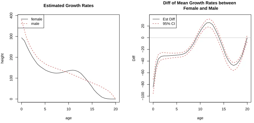
Figure 5 displays the estimated mean growth curves on the left panel and the difference

function along with 95% credible interval on the right panel. Males older than 3 years are

significantly taller than females at the same age, and females younger than 3 years appear

to be taller than males. Figure 6 shows the estimated growth rates as well as the difference

of growth rates between the two groups. It is not surprising to find that females are growing

significantly faster than males between age 10 to 14. However, before age 10 and from age

15 to age 18, males grow significantly faster.

6

Discussion

We proposed a class of linear mixed effects model using Bernstein polynomial sieve for fitting

longitudinal model under the assumption of Gaussian process. This nonparametric model

only requires very limited regularity conditions on the Gaussian process, and can incorporate

the shape restriction into the framework. With the proposed model, the derivative of the

response process can be easily obtained and its shape property can be retained as well.

Convergence properties of our proposed approximation are presented under a set of mild

regularity conditions. We also proposed a leave-one-out cross validation based Bayesian

model selection criterion, BPDC, which has been shown to have an explicit formula for

computation using the important sampling. Simulation studies were carried out to compare

that BPDC outperforms the other two in terms of selecting the correct model out of a class

of mixed effects models when a BPS is used. In the real data analysis, we applied our

methodology to the growth data of males and females. The nondecreasing constraint of

the growth curve was imposed in our proposed model using a linear transformation. The

coefficient of determination is demonstrated to be as high as 0.99, for the Berkeley growth

study. Interesting findings were revealed in looking at the growth curve estimates as well as

the growth rate estimates.

In the future, we would like to explore the longitudinal data subject to missing and

censored observations. Also, in our proposed model, we have concentrated on the simple

case where predictor z is not allowed to vary with time. We would like to investigate the

case where we have a time-varying Z(t) as our predictors.

References

Carnicer, J. and Pena, J. (1993). Shape preserving representations and optimality of the

Bernstein basis. Advances in Computational Mathematics, 1(2):173–196.

Chiou, J., M¨uller, H., and Wang, J. (2003). Functional quasi-likelihood regression models

with smooth random effects. Journal of the Royal Statistical Society: Series B (Statistical

Methodology), 65(2):405–423.

Crainiceanu, C. M. and Goldsmith, A. J. (2010). Bayesian functional data analysis using

winbugs. Journal of Statistical Software, 32(11):1–33.

Davidian, M. and Giltinan, D. (1995). Nonlinear models for repeated measurement data,

volume 62. Chapman & Hall/CRC.

overview and update. Journal of Agricultural, Biological, and Environmental Statistics,

8(4):387–419.

Davies, S. L., Neath, A. A., and Cavanaugh, J. E. (2005). Cross validation model

selec-tion criteria for linear regression based on the Kullback-Leibler discrepancy. Statistical

Methodology, 2(4):249–266.

Di, C., Crainiceanu, C., Caffo, B., and Punjabi, N. (2009). Multilevel functional principal

component analysis. Annals of Applied Statistics, 3(1):458–488.

Fasshauer, G. E. and McCourt, M. J. (2012). Stable evaluation of gaussian radial basis

function interpolants. SIAM Journal on Scientific Computing, 34(2):A737–A762.

Gal, S. (2008). Shape-preserving approximation by real and complex polynomials. Birkh¨auser

Boston.

Geisser and Eddy, W. F. (1979). A predictive approach to model selection. Journal of the

American Statistical Association, 74(365):153–160.

Gelfand, A. and Dey, D. (1994). Bayesian model choice: asymptotics and exact calculations.

Journal of the Royal Statistical Society. Series B (Methodological), 56(3):501–514.

Han, C. and Chaloner, K. (2004). Bayesian experimental design for nonlinear mixed-effects

models with application to hiv dynamics. Biometrics, 60(1):25–33.

Harville, D. (1977). Maximum likelihood approaches to variance component estimation and

to related problems. Journal of the American Statistical Association, 72(358):320–338.

Hoeffding, W. (1971). The l1 norm of the approximation error for Bernstein-type

Holsclaw, T., Sans´o, B., Lee, H. K., Heitmann, K., Habib, S., Higdon, D., and Alam, U.

(2013). Gaussian process modeling of derivative curves. Technometrics, 55(1):57–67.

Jones, D. H. (1976). The l2 norm of the approximation error for Bernstein polynomials.

Journal of Approximation Theory, 18:305–317.

Ke, C. and Wang, Y. (2001). Semiparametric nonlinear mixed-effects models and their

applications. Journal of the American Statistical Association, 96(456):1272–1298.

Kelisky, R. and Rivlin, T. (1967). Iterates of Bernstein polynomials. Pacific Journal of

Mathematics, 21(3):511–520.

Khan, R. A. (1985). On thelp norm for some approximation operators. Journal of

Approx-imation Theory, 45:339–349.

Laird, N. M. and Ware, J. H. (1982). Random-effects models for longitudinal data.

Biomet-rics, 38(4):963–974.

Lesaffre, E. and Lawson, A. B. (2012). Bayesian Biostatistics. Wiley.

Lindstrom, M. (1995). Self-modelling with random shift and scale parameters and a free-knot

spline shape function. Statistics in Medicine, 14(18):2009–2021.

Lindstrom, M. and Bates, D. (1988). Newtonraphson and em algorithms for linear

mixed-effects models for repeated-measures data.Journal of the American Statistical Association,

83(404):1014–1022.

Lorentz, G. G. (1953). Bernstein polynomials. Chelsea Publishing Co., New York, second

edition.

times using a piecewise nonlinear mixed-effects model in men with prostate cancer.Journal

of the American Statistical Association, 90(429):45–53.

Patterson, H. and Thompson, R. (1971). Recovery of inter-block information when block

sizes are unequal. Biometrika, 58(3):545–554.

Peruggia, M. (1997). On the variability of case-deletion importance sampling weights in the

Bayesian linear model. Journal of the American Statistical Association, 92(437):199–207.

Ritter, K., Wasilkowski, G. W., and Wo´zniakowski, H. (1995). Multivariate integration

and approximation for random fields satisfying sacks-ylvisaker conditions. The Annals of

Applied Probability, 5(2):518–540.

Robinson, G. (1991). That blup is a good thing: The estimation of random effects.Statistical

Science, 6(1):15–32.

Serroyen, J., Molenberghs, G., Verbeke, G., and Davidian, M. (2009). Nonlinear models for

longitudinal data. The American Statistician, 63(4):378–388.

Solak, E., Murray-Smith, R., Leithead, W., Leith, D., and Rasmussen, C. (2003). Derivative

observations in gaussian process models of dynamic systems. In Becker, S., Thrun, S., and

Obermayer, K., editors,Conference on Neural Information Processing Systems, Advances

in neural information processing systems 15. MIT Press.

Spiegelhalter, D. J., Best, N. G., Carlin, B. P., and van der Linde, A. (2002). Bayesian

measures of model complexity and fit (with discussion). Journal of the Royal Statistical

Society, Series B, 64(4):583–639.

Staicu, A., Crainiceanu, C., and Carroll, R. (2010). Fast methods for spatially correlated

Tenbusch, A. (1997). Nonparametric curve estimation with Bernstein estimates. Metrika,

45(1):1–30.

Vehtari, A. and Lampinen, J. (2002). Bayesian model assessment and comparison using

cross-validation predictive densities. Neural Computation, 14(10):2439–2468.

Wang, J. and Ghosh, S. (2012). Shape restricted nonparametric regression with Bernstein

polynomials. Computational Statistics & Data Analysis, 56(9):2729–2741.

Wu, H. and Ding, A. (1999). Population hiv-1 dynamics in vivo: Applicable models and

● ●

● ●

● ●

● ●●

●●●●●●●●●

●●●●●●●●●●●●●●●●●●●●●●●●●●●●●●●●●

0 10 20 30 40 50

0.0

0.5

1.0

1.5

2.0

2.5

3.0

Square Expentential Kernel

m

sum_0^m lambda_kV_1(e_k)

Figure 1: Pm i=0

√

Table 1: Percentage of model selection decisions over 200 repetitions

m BPDC LPML DICm DICc

Case 1 (m=4)

2 0 0 0 0

3 0 0 0 0

4 96.0 82.5 83.5 64.0

5 3.5 11.5 10.0 18.0

6 0 1.5 2.5 4.5

7 0.5 2.0 2.0 6.0

8 0 2.0 1.5 2.5

9 0 0.5 0.5 2.5

10 0 0 0 1.0

11 0 0 0 0.5

12 0 0 0 1.0

13 0 0 0 0

Case 2 (m=3)

2 0 0 0 0

3 76.5 58.5 59.5 43.0

4 13.0 19.5 19.0 24.0

5 7.0 10.5 11.0 15.0

6 3.5 11.5 10.5 18.0

Case 3 (m=3)

2 0 0 0 0

3 75.0 63.0 26.5 28.5

4 15.0 18.0 19.0 22.5

5 8.0 14.0 20.0 19.5

6 2.0 5.0 34.5 29.5

a_{BPDC: Bayesian predictive divergence criterion;}

LPML: log pseudo marginal likelihood; DICm: marginal deviance information criterion; DICc: conditional marginal deviance information crite-rion.

b_{The true value ofmis specified in the parentheses.} c_{The maximum value of each column for every case}

Table 2: Fit of Gaussian process with nonlinear mean and covariance functions

IBias(ˆµ) SE of IBias(ˆµ) p-value IBias( ˆK) SE of IBias( ˆK) p-value

0.0046 0.0077 0.5509 -0.0115 0.0085 0.1776

0.0 0.2 0.4 0.6 0.8 1.0

0

50

100

150

LMM−BP approxmiates nonlinear GP

x

m

u (x)

true estimated 95% CI

Figure 2: Estimated mean function is plotted in dashed red along with its pointwise 95% credible interval in dashed green lines. The true mean curve is displayed in solid black line.

5 10 15

80

100

120

140

160

180

200

Growth Data

age

height(cm)

female male

● ● ● ● ● ● ● ● ● ● ● ● ● ●

2 4 6 8 10 12 14

6000 7000 8000 9000 10000 11000 BPDC Female Group m BPDC ● ● ● ● ● ● ● ● ● ● ● ● ●

2 4 6 8 10 12 14

5000 5500 6000 6500 7000 BPDC Male Group m BPDC

Figure 4: BPDC of models for female and male group.

0 5 10 15 20

60 80 100 120 140 160 180 200

Estimated Growth Curves

age

height

female male

0 5 10 15 20

−20 −15 −10 −5 0 5

Diff of Mean between Female and Male

age

Diff

Est Diff 95% CI

0 5 10 15 20

0

100

200

300

400

Estimated Growth Rates

age

height

female male

0 5 10 15 20

−100

−80

−60

−40

−20

0

20

Diff of Mean Growth Rates between Female and Male

age

Diff

Est Diff 95% CI

Figure 6: Left: estimated mean function of growth rate over ages. Right: estimated difference function of growth rate and its 95% credible interval and the grey line is the references line at y=0.

Appendices

A

Proof of Theorem 1

Proof. By K-L expansion, with eigenvalues λ1 ≥λ2 ≥. . .≥0 and corresponding

eigenfunc-tions {ei(t), i= 1,2, . . .} the Gaussian process X(t) can be represented as an infinite series

such that X(t) =µ(t) +P∞ i=1

√

λiei(t)Zi in mean square sense, where Zi iid

∼N(0,1).

Xm(t) has the form of BTm(t)βm, where βm ∼ N(µm, Dm). Thus, we can write it in an

equivalent way such that Xm(t) = BmT(t)µm +BmT(t)D 1/2

m Z, where Z = (Z1, . . . , Zm)T. By

Bernstein Weierstrass approximation theorem, for any continuous function f, there exists

f−relatedm×1 vector γm(f) = (f(0), f(_m1₋₁), . . . , f(1))T such that BmT(t)γm(f) converges

(√λ1γm(e1), . . . ,

√

λmγm(em)). Then, Xm(t) = BmT(t)γm(µ) +Pm_i=1

√

λiBmT(t)γm(ei)Zi. So

EkX−Xmk22

= E[

Z 1

0

(X(t)−Xm(t))2dt],

=

Z 1

0

E{[µ(t)−B_mT(t)γm(µ)] + [

∞

X

i=1 p

λiei(t)Zi− m X

i=1 p

λiBmT(t)γm(ei)Zi]}2dt,

=

Z 1

0

[µ(t)−B_mT(t)γm(µ)]2dt

+ Z 1 0 E{ m X i=1 p

λi[ei(t)−BTm(t)γm(ei)]Zi+

∞

X

i=m+1 p

λiei(t)Zi}2dt,

=

Z 1

0

[µ(t)−B_mT(t)γm(µ)]2dt

+ Z 1 0 m X i=1

λi|ei(t)−BmT(t)γm(ei)|2dtE(Zi2) + Z 1

0

∞

X

i=m+1

λie2i(t)dtE(Z 2 i),

= kµ−B_mTγm(µ)k22+ m X

i=1

λikei−BmTγm(ei)k22+

∞

X

i=m+1

λikeik22.

By Bernstein Weierstrass approximation theorem, we have kµ −BT

mγm(µ)k22 ≤ kµ−

B_mTγm(µ)k2∞goes to 0 as m goes to infinity. Sinceλikei−BmTγm(ei)k22 is always nonnegative,

Pm

i=1λikei − BmTγm(ei)k22 ≤ P∞

i=1λikei −BmTγm(ei)k22 = m

−1P∞

i=1λimkei − BmTγm(ei)k22.

Define Q2

m(f) = R1

0 Pm

k=1|f( k−1

m−1)−f(t)| 2_b

m,k(t)dt, where bm,k(t) = m_k−−₁1

tk−1_(1−t)m−k_.

Then since Pm

k=1bm,k(t) = 1,

|ei −BmTγm(ei)|2 = | m X

k=1

ei(

k−1

m−1)bm,k(t)−ei(t)|

2_,

= |

m X

k=1

{ei(

k−1

m−1)−ei(t)}bm,k(t)|

2_,

≤

m X

k=1

|{ei(

k−1

m−1)−ei(t)}

q

bm,k(t)|2 m X

k=1

|qbm,k(t)|2,

=

m X

k=1

|ei(

k−1

m−1)−ei(t)|

2

using Cauchy-Schwarz inequality. Therefore,

kei−BmTγm(ei)k22 = Z 1 0 | m X k=1

ei(

k−1

m−1)bm,k(t)−ei(t)|

2_dt, ≤ Z 1 0 m X k=1

|ei(

k−1

m−1)−ei(t)|

2_b

m,k(t)dt=Q2m(ei).

Using Theorem 1 in Khan (1985), we have limm→∞mkei−BmTγm(ei)k22 ≤limm→∞mQ2_m(ei) =

C2V2(ei), whereV2(ei) = R1

0 t(1−t)|e

0

i(t)|2dt. Then, with assumption that P∞

i=1λiV2(ei)<∞

and Fatou’s lemma,

lim

m→∞ ∞

X

i=1

λimkei−BmTγm(ei)k22 ≤ _mlim_→∞

∞

X

i=1

λimQ2m(ei),

= C2

∞

X

i=1

λiV2(ei)<∞.

Thus, it follows that limm→∞Pm_i=1λikei−BmTγm(ei)k22 = 0. Meanwhile, with continuous

co-variance functionK, we haveP∞ i=1λi =

R1

0 K(t, t)dt <∞. Therefore, limm→∞ P∞

i=m+1λikeik22 =

limm→∞P∞_i=m+1λi = 0. Altogether, we have proved limm→∞EkX−Xmk22 = 0.

Remark: Notice that in the above proof the theorem can be extended even if X(t) is not

assumed to be a Gaussian process. Any second order process can be approximated using

Xm(t) as long as we know the distribution of the uncorrelated sequence of Zi’s satisfying

E(Zi) = 0 and Cov(Zi, Zi0) =δ_ii0.

B

Proof of Theorem 2

Proof. Using Mercer’s theorem , we haveX(t)=d µ(t)+P∞ i=1

√

λiei(t)Zi, whereZi iid

∼N(0,1).

Then we construct Xm(t) in the same way as we do in the proof of Theorem 1, say,

Xm(t) = BmT(t)µm +BmT(t)D 1/2

(√λ1γm(e1), . . . ,

√

λmγm(em)). Then,

EkX−Xmkp

= E{kµ(t) +

∞

X

i=1 p

λiei(t)Zi−BmT(t)γm(µ)− m X

i=1 p

λiBmT(t)γm(ei)Zikp},

≤ kµ−BT_mγm(µ)kp+ m X

i=1 p

λikei−BmTγm(ei)kpE|Zi|+

∞

X

i=m+1 p

λikeikpE|Zi|.

SinceZi ∼N(0,1), E|Zi|= pπ

2. By Bernstein Weierstrass approximation theorem, we have

limm→∞kµ−BT_mγm(µ)kp = 0. Define Qpm(f) = R1

0 Pm

k=1|f( k−1

m−1)−f(t)| p_b

m,k(t)dt, where

bm,k(t) = m_k−−₁1

tk−1(1−t)m−k. Theorem 1 in Khan (1985) implies that limm→∞

√

m{Qp_m(ei)}1/p=

Cp{Vp(ei)}1/p for some constant Cp which only depends on p. Because E|X| ≤ {E|X|p}1/p

forp≥1, we have|E(X)|p _≤E|X|p_{. So,|}Pm k=1{ei(

k−1

m−1)−ei(t)}bm,k(t)|

p _≤Pm k=1|f(

k−1 m−1)−

ei(t)|pbm,k(t)dt, since Pm

k=1bm,k(t) = 1. Hence,

kei−BmTγm(ei)kp = { Z 1 0 | m X k=1

ei(

k−1

m−1)bm,k(t)−ei(t)|

p_dt}1/p_,

≤ { Z 1 0 m X k=1

|ei(

k−1

m−1)−ei(t)|

p_b

m,k(t)dt}1/p,

= {Qp_m(ei)}1/p.

Then, lim m→∞ m X i=1 p

λikei−BmTγm(ei)kp ≤ lim m→∞m

−1/2 m X i=1 p λi √

m{Qp_m(ei)}1/p,

≤ lim

m→∞m −1/2 ∞ X i=1 p λi √

m{Qp_m(ei)}1/p.

Hence, with condition (i) such thatP∞ i=1

√

λi{Vp(ei)}1/p<∞, we have limm→∞P∞_i=1

√ λi

√

mkei−

B_mTγm(ei)kp ≤P

∞

i=1

√

λi{Vp(ei)}1/p <∞. Therefore, limm→∞Pm_i=1

√

λikei−BmTγm(ei)kp =

0. Together with condition (ii) such thatP∞ i=1

√

λikeikp <∞, we have proved limm→∞EkX−