On convergence of the immersed boundary method for elliptic
interface problems
Zhilin Li
∗January 26, 2012
Abstract
Peskin’s Immersed Boundary (IB) method is one of the most popular numerical methods for many years and has been applied to problems in mathematical biology, fluid mechanics, material sciences, and many other areas. Peskin’s IB method is associated with discrete delta functions. It is believed that the IB method is first order accurate in theL∞
norm. But almost no rigorous proof could be found in the literature until recently [14] in which the author showed that the velocity is indeed first order accurate for the Stokes equations with a periodic boundary condition. In this paper, we show first order convergence with a loghfactor of the IB method for elliptic interface problems essentially without the boundary condition restrictions. The results should be applicable to the IB method for many different situations involving elliptic solvers for Stokes and Navier-Stokes equations.
keywords: Immersed Boundary (IB) method, Dirac delta function, convergence of IB method, discrete Green function, discrete Green’s formula.
AMS Subject Classification 200065M12, 65M20.
1
Introduction
Since its invention in 1970’s, the Immersed Boundary (IB) method [15] has been applied almost everywhere in mathematics, engineering, biology, fluid mechanics, and many many more areas, see for example, [16] for a review and references therein. The IB method is not only a mathematical modeling tool in which a complicated boundary condition can be treated as a source distribution but also a numerical method in which a discrete delta function is used. The IB method is robust, simple, and has been applied to many problems.
∗
It is widely believed that Peskin’s IB method is only first order accurate in theL∞ norm.
How-ever, there was almost no rigorous proof in the literature until recently [14], in which the author has proved the first order accuracy of the IB method for the Stokes equations with a periodic boundary condition. The proof is based on some known inequalities between the fundamental solution and the discrete Green function with a periodic boundary condition for Stokes equations. In [4], the author showed that the pressure obtained from IB method hasO(h1/2) order of convergence in the
L2norm for a 1D model. In [19, 20], the authors designed some level set methods based on discrete
delta functions. With suitable quadrature formulas in the integral form using the Green functions, the authors show that their approach can get expected accuracy. However, there are few theoretical proofs on the IB method for elliptic interface problems with general boundary conditions. This is the main motivation of this paper. One difficult is that there is little known estimates between the fundamental solution and the discrete Green function with Dirichlet or other boundary conditions on rectangular domains. Compared with the case of periodic boundary conditions where there are existing estimates between the discrete Green function and the continuous one [8], there is almost none for Dirichlet and other boundary conditions. The main goal of this paper is to provide a con-vergence proof for the IB method for elliptic interface problems with Dirichlet boundary conditions. We will show that with commonly used discrete delta functions that satisfy the zeroth moment condition and first order interpolation property, the IB method is indeed first order convergent in theL∞ norm with a loghfactor. The key in our proof is to establish a connection between the
dis-crete Green function and the continuous one. Our proof is essentially independent of the boundary conditions and it is valid in 1D, 2D, and 3D cases. The result should be applicable for many IB methods involving Stokes and Navier-Stokes solvers.
2
Proof of the convergence of the IB method in 1D
We will give a proof for the 1D model,
u00=c δ(x−α) 0< x <1, 0< α <1, u(0) =u(1) = 0, (1)
first in this section. Note that the analytic solution to the equation above is
u(x) =
(
−cx(1−α) if x≤α,
−cα(1−x) otherwise. (2)
Given a uniform Cartesian grid xi =ih, i = 0,1,· · ·, n, h = 1/n, the IB method leads to the
following system of linear equations,
Ui−1−2Ui+Ui+1
h2 =cδh(xi−α), i= 1,2,· · · , n−1, (3)
whereUiis the finite difference approximation of the solutionu(xi), andδh(xi−α) is a discrete delta
function applied to the grid pointxi. In the matrix-vector form, the above finite difference equations
It is well known that−Ah is a symmetric positive definite matrix (SPD) and diagonally dominant.
Note that, a discrete delta function has a compact support in the neighborhood of interface, that is,
δh(x)6= 0 only if|x| ≤W h, whereW is a constant. Commonly used discrete delta functions include
the hat discrete delta function (δhat(x) withW = 1):
δhath (x) = (
(h− |x|)/h2, if|x|< h,
0, if|x| ≥h, (4)
and Peskin’s original discrete cosine delta function (δcosine(x) withW = 2)
δh(x)cosine=
1
4h(1 + cos (πx/2h)), if|x|<2h,
0, if|x| ≥2h.
(5)
see for example, [13]. Note that, when we use the hat delta function, the result is the same as that of the IIM for the simple model. The solution to the finite difference equations is the same as true solution if there are no round-off errors, that is
u(xi−1)−2u(xi) +u(xi+1)
h2 =cδ
hat
h (xi−α), i= 1,2,· · ·, n−1, (6)
see for example, [3, 13]. But this is not the case for other discrete delta functions.
We define the error vector as E={Ei}, whereEi =u(xi)−Ui. The local truncation error is
defined asT={Ti},
Ti=
u(xi−1)−2u(xi) +u(xi+1)
h2 −cδh(xi−α). (7)
With the definition, we haveAhU=F,Ahu=F+T, and thereforeAhE=T. For the hat discrete
delta function, we have|Ti|= 0 for alli’s for the simple model. For the cosine discrete delta function
or other discrete delta functions, generally we have|Tj|=O(1/h) for a few grid points neighboring
the interfaceα, see Table 1 on page 19. So the interesting question is: Why is the IB method still first order accurate, that is,kEk∞=O(h)? To answer this question, we first introduce the following
lemma.
Lemma 2.1. LetAhy=ek andy0=yn= 0, whereek is the k-th unit base vector, then
yi= (
−hxi(1−xk) if i≤k, −hxk(1−xi) otherwise.
(8)
The significance of this lemma is that the solution is order h smaller than the concentrated source.
Proof: We note the following identity
Ahy=h
ek
h =h δ
hat
For this simple case, the IB method using the hat discrete delta function is identical to the IIM, see [13]. Thus from the Immersed Interface Method, see [3, 13], we know thatyis the exact discrete solution at the grid points of the following boundary value problem
u00=h δ(x−xk), 0< x <1, u(0) =u(1) = 0, (10)
whose solution is
y(x) =
(
−hx(1−xk) if x≤xk, −hxk(1−x) otherwise.
(11)
This completes the proof. Note that|y(x)| ≤h. From this lemma, we have the following corollary.
Corollary 2.2. LetAhy=r, then |y(x)| ≤h Wkrk∞, where W is the number of non-zero compo-nents ofr.
The proof is straightforward from (11) and the fact that 0≤x ≤1 and 0≤1−x≤1. Notice that for a discrete delta function, it should satisfy at least the zeroth moment equation, see [3], that is
X
i
δh(xi−α) = 1, (12)
corresponding to the continuous case R
δh(x−α)dx = 1. Now we are ready to prove the main
theorem.
Theorem 2.3. Letu(x) be the solution to (1) and U is the solution obtained from the immersed boundary method (3) using a discrete delta function δh(x)for (1). Then U is first order accurate,
that is
kEk∞≤Ch,¯ (13)
whereC¯ is a constant.
Proof: We can decompose the local truncation error into two groups
T=Treg+Tirreg, (14)
wherekTregk∞= 0 corresponds to the local truncation errors at regular grid points whereδh(xi−
α) = 0 and the true solution is piecewise linear. Note that, we have
n−1
X
i=1
Ti= X
Treg+XTirreg =O+XTirreg. (15)
On the other hand, we also have
u(xi−1)−2u(xi) +u(xi+1)
h2 =cδ
hat
since the finite difference method using the discrete delta function gives the exact solution at all the grid points. Thus we have
n−1
X
i=1
Ti = u(xi−1)−2u(xi) +u(xi+1)
h2 −cδh(xi−α)
=
n−1
X
i=1
cδhat
h (xi−α)−
n−1
X
i=1
cδh(xi−α) = 0,
(17)
from the zeroth moment equation (12). Thus we have P iT
irreg
i = 0. We divide T irreg
i into two
groups, one with all positiveTi’s denoted asTiirreg,+; the other one is all the negatives denoted as
Tiirreg,−. Since PTirreg,+
i +
PTirreg,−
i = 0, T
irreg,+
i and T
irreg,−
i must have the same order of
the magnitudeO(1/h) although those indexiare different except that|xi−α| ≤W his true for all
irregular grid points. Because the solution is linear withc, we have
E=A−h1T=Ah−1 Tirreg,++Tirreg,−
. (18)
From the solution expression, we know that, assuming thatxl≤α,
El = A−h1T=Ah−1 Tirreg,++Tirreg,−
= −xl
X
i
Tiirreg,+(1−xi) + X
j
Tjirreg,−(1−xj)
= −xl(1−α)
X
i
Tiirreg,++ X
j
Tjirreg,−
+O(W h)
= O(W h),
after we expand allxi’s andxj’s at αand since all relatedxi andxj are withinW hdistance from
the interfaceα. The proof for xl > αis similar except that we need to use the solution forx > α.
This completes the proof.
3
Proof of the convergence of the IB method in 2D
0 0.1 0.2 0.3 0.4 0.5 0.6 0.7 0.8 0.9 1 0
0.1 0.2 0.3 0.4 0.5 0.6 0.7 0.8 0.9 1
Γ Ω+
Ω−
Ω=Ω+∪Ω−∪Γ
∂Ω
Figure 1: A diagram of a 2D elliptic interface problem. The interface is Γ.
Consider the following 2D elliptic interface problem,
∆u(x, y) =f(x, y) +R
Γv(s)δ(x−X(s)) (y−Y(s))ds, (x, y)∈Ω,
u(x, y)|∂Ω=u0(x, y),
(19)
where we assume thatf ∈C(Ω), Γ∈C1,v(s)∈C1. Without loss of generality, we assume that Ω
is a unit square 0≤x, y≤1, see Fig. 1 for an illustration. The problem can be decomposed as the sum of the solutions of the following two problems. The first one is
∆u1(x, y) =f(x, y)
u1(x, y)|∂Ω =u0(x, y),
(20)
which is a regular problem whose solutionu1(x, y)]∈C2(Ω). The second problem is
∆u2(x, y) =
Z
Γ
v(s)δ(x−X(s)) (y−Y(s))ds,
u2(x, y)|∂Ω = 0.
(21)
The solution to the second problem is equivalent to the following problem
∆u2(x, y) = 0, [u2]Γ = 0,
∂u2
∂n
Γ
=v(s),
u2(x, y)|∂Ω = 0.
The solution to the original problem isu=u1+u2. Sinceu1 is the solution to a regular problem,
it is enough just to consideru2(x, y). Thus we will simply use the notationu(x, y) foru2(x, y).
Peskin’s IB method for the problem includes the following steps:
• Generate a uniform Cartesian meshxi=ih,yj =jh, i, j= 0,1,· · ·, n. Here we use a uniform
mesh for simplicity. We denote Ωhas the set of all grid points; and∂Ωh as the grid points on
the boundary.
• Replace the partial derivatives with the finite difference approximation and use a discrete delta function to spread the singular source to nearby grid points
Ui−1,j+Ui+1,j +Ui,j−1+Ui,j+1−4Uij
h2 =C
IB
ij , i, j= 1,2,· · ·, n−1,
CijIB = Nb X
k=1
vkδh(xi−Xk)δh(yj−Yk) ∆sk,
(23)
where (Xk, Yk),k= 1,2,· · · , Nb, is a discretization of the interface Γ, and vk ≈v(sk), which
we assume it is at least first order approximation,vk=v(sk) +O(h).
• Solve the finite difference system of equations above to get an approximation solution{Uij}.
This can be done by calling a fast Poisson solver, say [1].
3.1
Discrete delta functions and discrete Green functions
As a common practice, we assume that maxk{sk}= ∆s∼O(h). In Peksin’s IB method, a discrete
delta function is used for two purposes. One is to spread the singular source to the nearby grids. The other one is to interpolate a grid function, say the velocity, to get its values on the interface. Thus the discrete delta function used should satisfies at least the zeroth moment condition as described in [3]. The interpolation using the discrete delta function should be at least first order accurate, that is,
n−1
X
i,j=1
h2
Nb X
k=1
vkδh(xi−Xk)δh(yj−Yk) ∆sk = Z
Γ
v(s)ds+O(h), (24)
which corresponds to
Z Z
Ω
Z
Γ
v(s)δ(x−X(s))δ(y−Y(s))dsdxdy=
Z
Γ
v(s)ds. (25)
FromRR
Ωu(x, y)δ(x−X)δ(y−Y)dxdy=u(X, Y), we should also have the interpolation property,
n−1
X
i,j=1
h2u(x
In (24) and (26), the error terms depend on the first order derivatives ofv(s) andu(x, y), respectively. The discrete delta function has a compact support, that is,
δh(xi−Xk) = 0, if|xi−Xk|> W h, and δh(yj−Yk) = 0, if|yj−Yk|> W h, (27)
wherexij = (xi, yj), andW is a constant.
We define the error vector asE={Eij}, whereEij =u(xi, yj)−Uij. The local truncation error
is defined asT={Tij},
Tij =
u(xi−1, yj) +u(xi+1), yj) +u(xi, yj−1) +u(xi, yj+1)−4u(xi, yj)
h2 −C
IB
ij . (28)
In the matrix vector form, we haveAhU=F,Ahu=F+T, and thereforeAhE=T, whereAh is
the matrix formed by the discrete Laplacian. We have|Tij|=O(h2) at regular grid points where
CIB
ij = 0. In general, we have |Tij| = O(1/h) for grid points neighboring the interface Γ except
for the correction terms using the Immersed Interface Method (IIM) [11, 12, 13] for which we have
|TIIM
ij | = O(h) at irregular grid points where the interface cuts through the standard five-point
stencil.
It is interesting that the local truncation errors can have orderO(1/h) at some grid points, but the global error is still ofO(h). There has to be some kind of cancelations of the errors, which can be seen from our proof process.
Definition 3.1. Letelm be the unit grid function whose values are zero at all grid points except at
xlm = (xl, ym) where its component is elm = 1. The discrete Green function centered atxlm with
homogeneous boundary condition is defined as
Gh(xij,xlm) =
(Ah)−1elm
1
h2
ij
, Gh(∂Ωh,xlm) = 0, (29)
where∂Ωh denotes the grid points on the boundary∂Ω.
Note that from Remark 4.4.6 in [7], we know thatGh(xij,xlm) is symmetric,
Gh(xij,xlm) =Gh xlm,xij
. (30)
The usual discrete Green function, also called a discrete fundamental solution, on the entire integer lattice is defined as
∆hgh(xij,xlm) =
1
h2, ifxij =xlm,
0, otherwise,
(31)
for all integersiandj, see for example, [2, 6, 7, 10, 14, 17, 18] for more discussions about the discrete Green’s functions. Note thatgh(xij,xlm) is also symmetric, that is,gh(xij,xlm) =gh(xlm,xij).
Lemma 3.2. The discrete first Green’s formula and an error estimate.
Letu(x, y) be the solution to (19). Thusu(x, y)is in the piecewise C1(Ω) space, that is, u(x, y)∈
C1(Ω\Γ); Assuming that the distance betweenΓand∂ΩisO(1), that is,dist(Γ, ∂Ω)∼O(1), then
we have
n−1
X
i,j=1
∆hu(xi, yj)h2= Z
∂Ω
∂u
∂nds+O(h) =
Z
Γ
v(s)ds+O(h), (32)
where
∆hu(xi, yj) =
u(xi−1, yj) +u(xi+1), yj) +u(xi, yj−1) +u(xi, yj+1)−4u(xi, yj)
h2 , (33)
is the discrete Laplacian using the standard five-point stencil, and the summation is over all the interior grid points.
Proof: We first prove the discrete first Green’s formula by expanding the summation. After cancelation of interior terms, only boundary terms are left in the summation as follows,
X
ij
∆hu(xi, yj)h2 = n−1
X
j=1
hu(x0, yj)−u(x1, yj)
h +
n−1
X
j=1
hu(xn, yj)−u(xn−1, yj) h
+
n−1
X
i=1
hu(xi, y0)−u(xi, y1)
h +
n−1
X
i=1
hu(xi, yn)−u(xi, yn−1) h
=
Z
∂Ω
∂u
∂nds+O(h).
On the other hand, by integrating both sides of the partial differential equation (19) withf(x, y) = 0 andu0(x, y) = 0, we get
Z Z
Ω
∆udxdy=
Z Z
Ω
Z
Γ
v(s)δ(x−X(s)) (y−Y(s))ds
dxdy, or equivalently, Z ∂Ω ∂u ∂nds=
Z
Γ
v(s)ds.
This completes the proof.
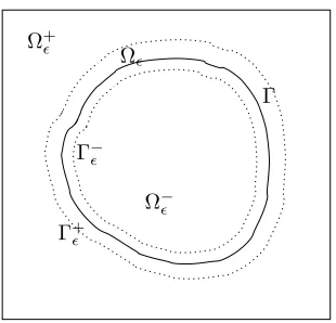
Remark 3.3. The double integral RR
Ω∆udxdy can be divided into three parts
Z Z
Ω
∆udxdy =
Z Z
Ω+
∆udxdy+
Z Z
Ω−
∆udxdy+
Z Z Ω ∆udxdy = Z ∂Ω ∂u ∂nds−
Z
Γ+
∂u ∂nds+
Z
Γ+
Ω+
Ω−
Γ−
Γ+
Ω
Γ
Figure 2: A diagram of the domain, interface, and integration.
see Fig. 2 for an illustration, see also [12]. As→0, we have
lim
→0
Z Z
Ω
∆udxdy=
Z
Γ
v(s)ds=
Z
Γ
∂u
∂n
ds
from the partial differential equation (19) withf(x, y) = 0andu0(x, y) = 0. Thus we get
lim
→0
Z Z
Ω
∆udxdy=
Z
∂Ω
∂u ∂nds.
While Lemma 3.2 is not directly used in our convergence proof, it is easier to illustrate the relation between the boundary integral along∂Ωand the source distribution alongΓfor the first Green formula than the second Green formula that is used in the proof.
3.2
Interpolating the discrete delta function
We know thatGh(xij,xlm) defined in (29) is a grid function with the homogeneous Dirichlet
bound-ary condition at the boundbound-ary grid points. The discrete Laplacian ∆hGh(xij,xlm) is zero at all
interior grid points except that it is 1/h2 at x
lm. We can interpolate Gh(xij,xlm) to the entire
domain to get an interpolation functionGh
I(x,xlm). We consider any such an interpolation function
that satisfies the following:
• GhI(xij,xlm) =Gh(xij,xlm).
• GhI(x,xlm)∈C1(Ω)∩H2(Ω).
• ∆hGhI(xij,xlm) = ∆hGh(xij,xlm) = 0, that is, zero for alliandjexcept fori=landj=m.
• The interpolation is second or higher order accurate, that is
∂αGh(xij,xlm)−∂αGhI(xij,xlm)
where the derivatives of Gh(xij,xlm) is defined from finite differences, see [18], and αis the
summation notation as used in the literature for the Sobolev spaces.
• RR
Rlm∆G
h
I(x,xlm)dxdy = O(h) except for the four neighboring squares centered atxlm on
whichRR
Rlm∆G
h
I(x,xlm)dxdy= 1 +O(h).
We provide a construction of such an interpolation function in Appendix.
Lemma 3.4. Let GhI(x,xlm)be an interpolation function of Gh(xij,xlm)that satisfies the
condi-tions above, then we have the following estimates:
G
h
I(x,xlm) ≤
1 4+
1
16log kx−xlmk
2 2+h2
+O(h), (35)
∂αGhI(x,xlm) ≤
C
(kxij−xlmk2+h)kαk1
+O(h), if kαk1≤k−1, (36)
wherekis the order of interpolation andCis a constant. The inequality (36) is true if dist(x, ∂Ω)∼ O(1) and dist(∂Ω,xlm)∼O(1).
Proof: From Remark 4.4.8 in [7], we know that
|Gh(xij,xlm)| ≤
1 4+
1
16log kx−xlmk
2 2+h2
.
Thus from the order requirement of the interpolation function, we have the first inequality. To prove the second inequality, we use the expression from (4.11) in [17]:
Gh(xij,xlm) =gh(xij,xlm)−sˆ(xij,xlm)−s(xij,xlm), (37)
where ˆs(xij,xlm) is chosen such that ∆hGh(xij,xlm) = 0 at the grid points on the boundary of
the unit square using the method of images. Thus ˆs(xij,xlm) is a combination of gh(xij,xlm)
at points outside of the unit square. From Theorem 3.1 in [18], we have |∂αg
h(xij,xlm)| ≤
C/(kxij−xlmk2+h)kαk1. The same can be said for ˆs(xij,xlm). The terms(xij,xlm) is chosen such
thatGh(xij,xlm) = 0 at the grid points on the boundary of the unit square and ∆hs(xij,xlm) = 0
at all other grid points. Thuss(xij,xlm)|∂Ωh is the trace ofgh(xij,xlm)−sˆ(xij,xlm), see Remark
on page 297 in [5]. Since the values ofs(xij,xlm)|∂Ωh are from the discrete Laplacian, it can be
smoothly extended to the entire boundary ∂Ω. Thus from Lemma 2.7.5 in [9] and the maximum principle, we have
∂
αs(x,x lm)
≤
C
kαk1
dist(x, ∂Ω)
kαk1
sup
Ω |
s|=
C
kαk1
dist(x, ∂Ω)
kαk1
sup
∂Ω |
s|, (38)
whereC is another constant. From Section 4.4 in [17], we know thats(xij,xlm) =O(1) as long as
dist(∂Ω,xlm) = O(1). Thus as long as dist(x, ∂Ω)∼ O(1), we have ∂αs(x,xlm) ∼O(1). This
Remark 3.5. The interpolation function is not unique. Along the boundary ∂Ω, from the require-ment of the interpolation function, ∂Gh
I(xij,xlm)/∂n does exist and continuous. We have, for
example
∂GhI(xij,xlm)
∂x =
GhI (x1j,xlm)−GhI(x0j,xlm)
h +O(h) (39)
along the boundaryx= 0.
By similar procedure in proving the discrete Green’s formula, we can get the second discrete Green’s formula.
Lemma 3.6. Let u(x, y) be the solution to (19) and GhI(x,xlm) be an interpolation function of
Gh(x
ij,xlm)that satisfies the conditions listed in Section 3.2. If l, m6= 1 orn−1, then we have,
X
ij
∆hu(xi, yj)Gh(xij,xlm)h2= Z
Γ
v(s)GhI(X(s),xlm)ds+O(h).
Proof: Again, we show the second discrete Green’s formula by expanding the summation. After cancelation of interior terms, only boundary terms and a source are left. Thus, we get
n−1
X
i,j=1
∆hu(xi, yj)Gh(xij,xlm)h2= n−1
X
j=1
hu(x0, yj)−u(x1, yj)
h G
h(x
1j,xlm)
+
n−1
X
j=1
hu(xn, yj)−u(xn−1, yj)
h G
h(x
n−1,j,xlm) + n−1
X
i=1
hu(xi, y0)−u(xi, y1)
h G
h(x i1,xlm)
+
n−1
X
i=1
hu(xi, yn)−u(xi, yn−1)
h G
h(x
i,n−1,xlm)− n−1
X
j=1
hG
h(x
0j,xlm)−Gh(x1j,xlm)
h u(x1, yj)
− n−1
X
j=1
hG
h(x
n,j,xlm)−Gh(xn−1,j,xlm)
h u(xn−1, yj)−
n−1
X
i=1
hG
h(x
i0,xlm)−Gh(xi1,xlm)
h u(xi, y1)
− n−1
X
i=1
hG
h(x
i,n,xlm)−Gh(xi,n−1,xlm)
h u(xi, yn−1) +
n−1
X
i,j=1
u(xi, yj)∆hGh(xij,xlm)h2
=
Z
∂Ω
∂u ∂n(x)G
h
I(x,xlm)−∂
Gh
I(x,xlm)
∂n u(x)
ds+u(xlm) +O(h).
On the other hand, by integrating both sides of the partial differential equation (19) withf = 0 and
u0= 0, we get
Z Z
Ω
GhI(x,xlm)∆udxdy= Z Z
Ω
Z
Γ
v(s)δ(x−X(s)) (y−Y(s))ds
GhI(x,xlm)dxdy,
or equivalently, Z ∂Ω ∂u ∂nG h
I(x,xlm)−∂
Gh
I(x,xlm)
∂n u
ds+
Z Z
Ω
u∆GhI(x,xlm)dxdy= Z
Γ
Note that
Z Z
Ω
u(x)∆GhI(x,xlm)dxdy= X
Rij\Rlm Z Z
Ω
u(x)∆GhI(x,xlm)dxdy+ Z Z
Rlm
u(x)∆GhI(x,xlm)dxdy
=X
Rij Z Z
Rij
u(xij) +O(h)
O(h)dxdy+
Z Z
Rlm
u(xlm) +O(h)
∆GhI(x,xlm)dxdy
=X
Rij
u(xij)O(h3) +u(xlm) Z Z
Rlm
∆GhI(x,xlm)dxdy+O(h)
=O(h) +u(xlm) +O(h) =u(xlm) +O(h),
whereRij is the square centered atxij. This completes the proof.
Lemma 3.7. LetCIB
ij be the correction terms in the immersed boundary method (23), v(s)∈ C1
be defined in (19), and GhI(x,xlm) be an interpolation function of Gh(xij,xlm) that satisfies the
conditions listed in Section 3.2. Then we have the following estimate.
X
ij
CijIBGh(xij,xlm)h2= Z
Γ
v(s)GhI(X(s),xlm)ds+O(hlogh).
Proof: We denotehs= max{∆sk} ∼h.
X
ij
CijIBGh(xij,xlm)h2= X
ij Nb X
k=1
vkδh(xi−Xk)δh(yj−Yk) ∆skGh(xij,xlm)h2
=
Nb X
k=1
vk∆sk X
ij
δh(xi−x)δh(yj−y)GhI(xij,xlm)h2
=
Nb X
k=1
vk∆sk GhI (Xk,xlm) +Ek
.
From the expression (4.2) and Lemma 4.1 in [3], we know that
|Ek| ≤Ch X
kαk1=1
∂αGhI(ξk,xlm).
The summation PNb
k=1vk∆sk GhI(Xk,xlm) +Ek is the composite trapezoidal rule for the line
integral. We divide the summation into three groups, one with the summation of k that kXk−
xlmk2≥
√
h, one withh≤ kXk−xlmk2≤
√
h, and the other is for the rest ofk’s. The contributions from the boundary points are split as half and half for each group. For the first two groups, we have
X
kXk−xlmk2≥h
00v
k∆sk GhI(Xk,xlm) +Ek=
Z
Γ−Γh
xlm
where00means the coefficients is half at the two boundary points. For the partkXk−xlmk2≥√h,
we have
Eh1
≤ Ch2smax k
1
(kXk−xlmk2+h)2
≤Ch2s
1
√
h+h2
≤Ch,
due to the second order partial derivatives ofGhI(X(s),xlm) and the first order derivatives ofEk.
For the part h≤ kXk−xlmk2 ≤
√
h, the error estimate is a little bit tricky. From the error estimate of the trapezoidal rule in each interval, we have
Eh1
≤
h2
s
12
X
k
hs X
kαk1=2
∂αGhI(ξk,xlm)≤Ch2s X
k
hs
kξk−xlm)k2+h 2
≤ Ch2s
Z √hs
hs
dr
r+h2 ≤Ch
2
s Z √hs
hs dr r2 ≤Ch.
For the last group, we have
X
kXk−xlmk2≤h
00v
k∆sk GhI (Xk,xlm) +Ek
=
Z
Γh
xlm
v(s)GhI (X(s),xlm)ds+E2h
≤ max
s v(s)hlogh+E
2
h,
from the estimate ofGh
I(X(s),xlm) in (36). For the error term Eh2, since the length of the integral
isO(h), we have
Eh2
≤Ch2hmax Xk
1
(kXk−xlmk2+h)2
≤Ch3 1
(h+h)2 ≤Ch.
This completes the proof of the lemma.
Now we are ready to prove the main result of the paper.
Theorem 3.8. Letu(x, y)be the solution to (19) andUis the solution obtained from the immersed boundary method (23) using a discrete delta functionδh(x)for (19). Then Uis first order accurate
with a logarithm factor in theL∞ norm, that is,
Proof: Consider the error at a grid point Elm, if xlm is close to the interface, that is,
dist(Γ,xlm)≤W h, we have
Elm = (Ah)−1TIBlm
= (Ah)−1TIBreg
lm+ (Ah)
−1TIB irr
lm
= O(h2) + (Ah)−1TIBirr
lm
= X
dis(xij,Γ)≤W h
h2Tij(Ah)−1eij
1
h2
lm
+O(h2)
= X
dis(xij,Γ)≤W h h2 ∆
hu(xi, yj)−CijIB
Gh(xij,xlm) +O(h2)
= X
ij
h2∆hu(xi, yj)Gh(xij,xlm)− X
ij
h2CijIBGh(xij,xlm) +O(h2)
=
Z
Γ
v(s)GhI(X(s),xlm)ds− X
k
vkGhI(Xk),xlm)∆sk !
+O(h)
= O(hlogh),
after we apply Lemma 3.6 and Lemma 3.7. Note that, in the expansion of the summation from
dis(xij,Γ)≤ W h to all interior grid points, we have used the fact that ∆hu(xi, yj) = O(h2) and
CIB
ij = 0 whendis(xij,Γ)> W h. Ifdist(Γ,xlm)> W h, the proof above is still valid except that we
are not going to have the singular integration. Thus, we do not need to have the loghfactor. This means that for IB method, the larger errors often occur near or on the interface.
4
Conclusions and acknowledgments
We give a convergence proof of the immersed boundary (IB) method in the L∞ norm. The key
of the proof is to establish a connection between the discrete Green function and a continuous one with the same boundary conditions. We show that the IB method is indeed first order accurate with a loghfactor if a reasonable discrete delta function is used. The conclusion should be applicable to other linear boundary conditions in addition to Dirichlet type as long as the method of images apply.
References
[1] J. Adams, P. Swarztrauber, and R. Sweet. Fishpack: Efficient Fortran subprograms for the solution of separable elliptic partial differential equations. http://www.netlib.org/fishpack/.
[2] J. T. Beale and A. T. Layton. On the accuracy of finite difference methods for elliptic problems with interfaces. Commun. Appl. Math. Comput. Sci., 1:91–119, 2006.
[3] R. P. Beyer and R. J. LeVeque. Analysis of a one-dimensional model for the immersed boundary method. SIAM J. Numer. Anal., 29:332–364, 1992.
[4] K.-Y. Chen, K.-A. Feng, Y. Kim, and M.-C. Lai. A note on pressure accuracy in immersed boundary method for stokes flow. J. Comput. Phys., 230:4377–4383, 2011.
[5] L. C. Evans. Partial Differential Equations. AMS, 1998.
[6] K. G¨urlebeck and A. Hommel. On finite difference potentials and their applications in a discrete function theory. Math. Meth. Appl. Sci., 25:1563–1576, 2002.
[7] W. Hackbusch. Elliptic Differential Equations: Theory and Numerical Treatment. Springer-Verlag, 1992.
[8] H. Hasimoto. On the periodic fundamental solutions of the Stokes equations and their applica-tion to viscous flow past a cubic array of spheres. J. Fluid Mech., 5:317–328, 1956.
[9] N. V. Krylov. Lectures on Elliptic and Parabolic Equations in Holder Spaces. AMS, 1996.
[10] G. F. Lawler. Intersections of random walks. Birkhauser, 1996.
[11] R. J. LeVeque and Z. Li. The immersed interface method for elliptic equations with discontin-uous coefficients and singular sources. SIAM J. Numer. Anal., 31:1019–1044, 1994.
[12] Z. Li.The Immersed Interface Method — A Numerical Approach for Partial Differential Equa-tions with Interfaces. PhD thesis, University of Washington, 1994.
[13] Z. Li and K. Ito. The Immersed Interface Method – Numerical Solutions of PDEs Involving Interfaces and Irregular Domains. SIAM Frontier Series in Applied mathematics, FR33, 2006.
[14] Y. Mori. Convergence proof of the velocity field for a Stokes flow immersed boundary method.
Comm. Pure Appl. Math., 61:2008, 1213-1263.
[15] C. S. Peskin. Numerical analysis of blood flow in the heart. J. Comput. Phys., 25:220–252, 1977.
[16] C. S. Peskin and D. M. McQueen. A general method for the computer simulation of biological systems interacting with fluids. Symposia of the Society for Experimental Biology, 49:265, 1995.
[18] V. Thom´ee. Discrete interior schauder estimates for elliptic difference operators. SIAM J. Numer. Anal., 5:626–645, 1968.
[19] A.-K. Tornberg and B. Engquist. Numerical approximations of singular source terms in differ-ential equations. J. Comput. Phys., 200:462–488, 2004.
[20] A.-K. Tornberg, B. Engquist, and R. Tsai. Discretization of Dirac delta functions in level set methods. J. Comput. Phys., 207:28–51, 2005.
[21] S. Zhang. On the full C1-Qk finite element spaces on rectangles and cuboids.Adv. Appl. Math. Mech., 2:701–721, 2010.
A
The construction of an interpolation function of the
dis-crete Green function
We construct an interpolation function from the grid function ∆GhI(xij,xlm) to of the discrete Green
function ∆Gh
I(x,xlm) that satisfies the conditions listed on page 10.
Letφ(x, y) be the function that satisfies the following conditions:
•
∆GhI(x,xlm) =δh(x, y),
Z Z
lm
δh(x, y)dxdy=
1
h2. (41)
• ∆GhI(x,xlm) takes values ofGhI(xij,xlm) at four corners and the center.
In other words, we choose the source term and the boundary condition so that the above two conditions are satisfied.
Then, we construct the interpolation function GhI(x,xlm) on other squares from the values of
∆Gh
I(x,xlm) usingQk(K)∈C1(Ω), whereQk is defined as the finite element space
Qk(K) =
v(x, y), on eachRˆiˆj:v(x, y) =
k X
i=0,j=0
βijxiyj, v(x, y)∈C1(Ω)
(42)
over a quadrilateral meshK,Rˆiˆj is a square ofhbyh. In the paper [21], the author has proposed
a system way to constructC1-Q
k finite element spaces on quadrilaterals meshes.
We have implemented and tested the interpolation functionGhI(x,xlm) ofQ5(K)∈C1(Ω), which
is third order accurate (k = 3). As usual, we just need to construct a shape function over a unit square. The total degree of freedom of Q5(K)∈C1(Ω) is 36. In our construction, we specify the
values ofv, vx, vy, vxx, vxy, vyy, which imposes 24 constraints. To keep the continuity of the solution
and first order partial derivatives, for example, along the sidex= 0, we impose the coefficients of
constraints. Using the undetermined coefficient method for the 36 constraint with the 32 conditions, we have a system of equations with 36 unknowns and 32 equations (constraints). The condition number of the coefficient matrix, the ration of the largest and smallest non-zero singular values is 8.9851× 10³, which indicates the matrix has full row rank and the system of equations has infinite
number of solutions. We suggest to choose the SVD solution as the interpolation function.
To see that the interpolation function is in C1, we use the side x = 0 as an example. Along
this side, the function is a fifth polynomial, which is uniquely determined by its values, the first and second order derivatives at two points. Thus the interpolation function and its tangential derivative are continuous along this side. The normal derivative is in general still a fifth polynomial ofyalong
x= 0. After we impose the constraints that its coefficients of xy5 andxy4 to be zero, it becomes a
cubic polynomial which is uniquely determined by its values (vx) and tangential derivatives (vxy) at
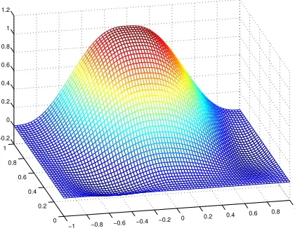
two points. In figure 3, we show a plot of such an interpolation function in two neighboring square with function value at one corner be a unit while others and all the derivatives are zero.
−1 −0.8 −0.6 −0.4 −0.2 0 0.2 0.4 0.6 0.8 1 0
0.2 0.4 0.6 0.8 1 −0.2
0 0.2 0.4 0.6 0.8 1 1.2
Figure 3: A plot of the shape function inQ5(K)∈C1(Ω) at two neighboring squares.
B
A numerical example
We use a numerical example to show that the immersed boundary method is indeed first order accurate and its local truncation error is of orderO(1/h). The differential equation is
∆u(x, y) =
Z
Γ
where the interface Γ is the circler= 1/2, wherer=px2+y2. The function
u(x, y) =
(
1 ifr≤ 1 2
1 + log(2r) ifr > 12 (44)
satisfies the PDE. This example is taken from [11]. We use the IB method to solve the PDE with the Dirichlet boundary condition given by (44). In Table 1, we list the results of a grid refinement analysis. In Table 1, the number N is the number of grid lines in the x and y directions. The interfacer= 1/2 is discretized byXk= 0.5 cos(2kπ/N)Yk = 0.5 sin(2kπ/N),k= 0,1,· · ·, N−1.
N kEcosk
∞ ordercos kTcosk∞ kEhatk∞ orderhat kThatk∞
20 5.7217 10−2 17.3534 2.1724 10−2 9.1327
40 2.7226 10−2 1.0715 34.9848 9.9933 10−3 1.1202 20.6630
80 1.3399 10−2 1.0228 69.9772 5.2761 10−3 0.9215 43.5721
160 6.7340 10−3 0.9926 139.254 4.5365 10−3 2.1789 117.289
320 3.3510 10−3 1.0066 279.483 1.8853 10−3 1.2667 195.664
640 1.6737 10−3 1.0018 556.360 1.1985 10−3 0.6536 495.791
1280 8.4663 10−4 0.88326 1122.01 5.4021 10−4 1.1497 892.463
Table 1: A grid refinement analysis of the IB method using discrete cosine and hat delta functions.
In the second and fifth columns of Table 1, we show the L∞ errors of the computed solution