DOI: 10.1534/genetics.108.090175
Practical Applications of the Bioinformatics Toolbox for Narrowing
Quantitative Trait Loci
Sarah L. Burgess-Herbert,
1Allison Cox, Shirng-Wern Tsaih and Beverly Paigen
2The Jackson Laboratory, Bar Harbor, Maine 04609 Manuscript received April 10, 2008 Accepted for publication October 1, 2008
ABSTRACT
Dissecting the genes involved in complex traits can be confounded by multiple factors, including extensive epistatic interactions among genes, the involvement of epigenetic regulators, and the variable expressivity of traits. Although quantitative trait locus (QTL) analysis has been a powerful tool for localizing the chromosomal regions underlying complex traits, systematically identifying the causal genes remains challenging. Here, through its application to plasma levels of high-density lipoprotein cholesterol (HDL) in mice, we demonstrate a strategy for narrowing QTL that utilizes comparative genomics and bioinformatics techniques. We show how QTL detected in multiple crosses are subjected to both combined cross analysis and haplotype block analysis; how QTL from one species are mapped to the concordant regions in another species; and how genomewide scans associating haplotype groups with their phenotypes can be used to prioritize the narrowed regions. Then we illustrate how these individual methods for narrowing QTL can be systematically integrated for mouse chromosomes 12 and 15, resulting in a significantly reduced number of candidate genes, often from hundreds to,10. Finally, we give an example of how additional bioinformatics resources can be combined with experiments to determine the most likely quantitative trait genes.
C
OMPLEX traits are the rule rather than the exception in nature, regardless of whether one’s scientific perspective originates within the realm of agriculture, ecology, medicine, or another biological discipline. Heritable phenotypic variation is the cor-nerstone of natural and artificial selection. Simple one-to-one relationships between traits and genes would yield predictable and easily manipulated outcomes. Indeed, farmers, horticulturists, and breeders have been manipulating the traits of organisms for millennia (Vila et al. 1997; Pringle 1998; Kislev et al. 2006). However, almost all traits are controlled by complex gene–gene and gene–environment interactions, and the predictable manipulation of the genes or gene products controlling them is anything but simple. Successful dissection of the individual genetic com-ponents of complex, or quantitative, traits will re-veal invaluable insights into their regulation and will provide targets for their manipulation. In addi-tion, since the investigation of proximate factors and the study of ultimate causes are complementary, this reductionist approach of dissecting out quantitative trait genes will likely prove to be a Rosetta stone forcomprehending the roles of adaptation, evolutionary legacy, and pleiotropy in maintaining variation within traits.
Model organisms facilitate the discovery of complex trait genes through classical experimental techniques and, more recently, through the application of bio-informatics resources and tools. For biomedical re-searchers, they also provide important models for many human diseases. Using model organisms, many complex traits of medical and agricultural importance have been mapped to chromosomal regions by quanti-tative trait locus (QTL) analysis (Moore and Nagle 2000; Peters et al. 2007). QTL mapping, based on classical forward genetics techniques together with statistical methodologies developed within the field of quantitative genetics, has succeeded in exposing the complex genetic architecture of many quantitative traits. For example, 38 QTL for drought resistance have been found in rice (Gramene: A Resource for Compar-ative Grass Genomics, Version 23, March 2008; http:// www.gramene.org; Jaiswal et al. 2005), at least 40 unique QTL for milk yield have been mapped in cows (QTL Map of Dairy Cattle Traits, March 2008; http:// www.vetsci.usyd.edu.au/reprogen/QTL_Map; Khatkar
et al. 2004), and 13 unique bone mineral density QTL have been mapped in rats (Rat Genome Database, March 2008; http://rgd.mcw.edu). However, despite the thousands of known QTL and the well-understood importance of elucidating their causal genes, relatively
Microarray data have been submitted to GEO accession no. GSE10493.
1Present address: Zoological Society of San Diego, Conservation and
Research for Endangered Species, Escondido, CA 92027.
2Corresponding author:600 Main St., Bar Harbor, ME 04609.
E-mail: [email protected]
few quantitative trait genes (QTGs) have been identified (Flintet al.2005). Much of the difficulty associated with proving QTGs lies in the prolonged and costly process of narrowing a QTL to a region with few enough candidate genes that each can be thoroughly tested.
This ability to reduce QTL to a small number of testable candidate genes will be essential for increasing the rate at which QTGs are identified and proven. We present here an effective strategy for narrowing QTL that harnesses the power of a variety of methods by combining results from experimental crosses with the newer bioinformatics tools and statistical methods reviewed recently (DiPetrilloet al.2005). We system-atically demonstrate the step-by-step integration of ex-perimentally determined QTL with combined cross results, haplotype block analyses, comparative genomics, and genomewide haplotype association mapping (HAM) using plasma levels of high-density lipoprotein choles-terol (HDL) in inbred lines of mice as an example complex trait.
The effectiveness of integrating these methods for narrowing QTL regions, and hence reducing candidate gene lists, is illustrated using two different mouse chromosomes as specific examples. Our analysis of mouse chromosome 12 illustrates the application and integration of all four bioinformatics tools, and our analysis of mouse chromosome 15 provides an example of the effectiveness of this strategy even when not all tools are applicable.
METHODS AND RESULTS
To visualize this integration of QTL-narrowing meth-ods, we first standardized a system for representing the different components of our analysis on chromosome maps. Here we represent the mouse chromosomes using one column per 1.0 Mb in Excel spreadsheets, but any program with the ability to manipulate in-formation in rows and columns would suffice. Alterna-tively, the genome browsers Ensembl (http://www. ensembl.org) and UCSC Genome Bioinformatics (http:// genome.ucsc.edu) include software that enables users to upload customized data sets, in a mutually compat-ible format, as additional annotation tracks (Kentet al. 2002; Hubbard et al. 2006; Kuhn et al. 2007). One advantage of using the genome browser tools is that the data set is automatically updated as new builds are released.
After constructing chromosome maps of appropriate lengths, we add the following: (1) the peak and 95% confidence intervals for all relevant QTL analyses, (2) the peak and 95% confidence intervals for combined cross analyses, (3) the regions where QTL of other species are homologous to the study organism’s QTL, (4) the results of haplotype block analyses, and (5) the results of HAM analyses. Figure 1 illustrates the results of this process for our two murine HDL QTL examples.
QTL mapping:HDL cholesterol is a highly complex trait, as evidenced by 40 unique QTL influencing plasma HDL levels in mice. These unique loci were estimated from the 111 HDL QTL identified by 23 different inbred line crosses (Rollinset al.2006). We placed the peak location and the 95% confidence intervals of each cross onto our chromosome maps. If published crosses reported no confidence intervals, we estimated them to be 20 cM surrounding the peak. Because genetic linkage positions (in centimorgans) from QTL analyses are based on recombination fre-quencies, precise conversion to physical positions (in megabases) is difficult to standardize. To standardize our conversion of centimorgans to megabases, first we created a publicly available database (http://cgd.jax.org) linking centimorgans to megabases in mice through MIT markers, commonly used sequence-tagged sites developed by the Whitehead Institute at MIT. Second, for the edges and peaks of our QTL and combined crosses, we averaged the megabase values for the relevant centimorgan positions and calculated their standard deviations. For the edges, we chose the most inclusive MIT marker within one standard deviation of the mean megabase value; for the peaks, we chose the MIT marker closest to the mean megabase value.
Figure 1A shows mouse chromosome 12 with its three known HDL QTL: 129S1/SvImJ3RIIIS/J (1293RIII) (Lyons et al.2004), C57BL/6J 3129S1/SvImJ (B6 3 129) (Ishimori et al. 2004), and RF/J 3 NZB/B1NJ (RF 3NZB) (Wergedal et al.2007). We also present mouse chromosome 15 (Figure 1B) with only its mid-region HDL QTL illustrated: MRL/lpr 3 BALB/cJ (MRL3BALB) (Guet al.1999). Although chromosome 15 has HDL QTL at its proximal, middle, and distal regions, we are presenting the mid-chromosome QTL alone to demonstrate both the limitations and the successes of using this integrated strategy for a QTL supported by only a single known cross.
Combined cross analysis:It is possible to combine the genotype and phenotype data from crosses that yield colocalized QTL (Liet al. 2005), the assumption being that the QTL from each cross are caused by the same underlying gene. By recoding the genotypes of the different crosses as ‘‘high,’’ ‘‘low,’’ and ‘‘heterozygous,’’ crosses genotyped with different markers can be com-bined using software such as Pseudomarker (http:// research.jax.org/faculty/churchill), MATLAB, or R/ QTL (http://www.rqtl.org; Senand Churchill 2001), and the QTL linkage analysis can be rerun using the combined data set. The polymorphisms used for geno-typing the crosses do not need to be the same because Pseudomarker, MATLAB, and R/QTL can infer the missing genotypes from adjacent markers and the re-combination frequencies. In addition, because the original cross-segregation data are needed to employ this powerful narrowing method, we encourage re-searchers to publicly archive their QTL data sets. (For mouse data, archive at http://research.jax.org/faculty/ churchill.)
This process of combining crosses increases statistical power. Therefore, when the assumption that the QTL are caused by the same gene is valid, the 95% confi-dence interval of the underlying unique QTL is typically narrowed. An excellent example was illustrated by DiPetrilloet al.(2005), where combining four crosses for an HDL QTL on chromosome 4 narrowed the QTL from 30 to 10 cM. However, sometimes the assumption is violated. In such cases, where the QTL are caused by
multiple genes, the increased statistical power of com-bining crosses may help discern that fact. For example, when multiple causal genes are shared by the QTL from different crosses, combining those crosses may reveal distinct multiple peaks, as illustrated by Ishimoriet al. (2008), where two crosses yielding a broad QTL for bone mineral density on chromosome 9 were com-bined, revealing two distinct peaks at cM 34 and cM 50. On the other hand, when the different cross QTL are caused by completely different genes, combining those crosses may fail to narrow or may even widen the 95% confidence interval. In any case, the exercise of com-bining the crosses of colocated QTL can be informative, as it may provide an indicator that one’s assumptions about those QTL are overly simplistic. If there is some indication that the QTL are caused by completely different genes, then one would hesitate to continue work based on those assumptions.
In our example, we combined the two crosses on chromosome 12 with publicly available data sets using MATLAB software (Figure 1A). The 330 samples from RIII3129 (LOD 5.1) plus the 294 samples from B63 129 (LOD 6.2) combined to yield a narrowed interval with a LOD score of 11.7. This reduced the QTL to a 26.3-Mb interval containing 135 genes.
Comparative genomics: Conservation of genes and proteins across a wide evolutionary spectrum validates the use of model organisms as indispensable tools for a broad array of queries in biology. For queries in the biomedical sciences, comparisons between rodents and
Figure
humans are especially useful, owing both to the rela-tively recent evolutionary split between the two lineages and to the extensive data already available on rodents. However, comparisons among a variety of organisms are increasingly tenable thanks to the recent explosion and continued growth of shared genome resources. Comparative genomics is therefore becoming a more useful and powerful tool for locating the genes un-derlying traits of interest across a range of biological disciplines.
In addition to our ever-increasing wealth of genome sequence data and published QTL studies, curated web-based resources for helping researchers directly com-pare syntenic regions across species are available and improving. In addition to the Rat Genome Database (http://rgd.mcw.edu) where comparisons among rat, mouse, and human QTL can be made, there are excellent resources within the field of agricultural genetics that also allow for the side-by-side comparison of QTL data across species. For example, the Animal QTLdb (http://www.animalgenome.org/QTLdb) is a comprehensive database that allows for the direct comparison of concordant QTL across genomes; it is currently limited to livestock (chickens, cows, pigs, and sheep), but is expected to expand to include rat, mouse, and human data as well (Zhi-Liangand James 2007). Gramene (http://www.gramene.org), another valuable resource, is a repository and tool for investigations of cereal genomes including rice, wheat, maize, sorghum, barley, rye, sugarcane, and other agriculturally impor-tant crop grasses ( Jaiswalet al.2006).
QTL have a high degree of concordance between mice and humans for plasma lipids (Wangand Paigen 2005), hypertension (Stollet al. 2000; Sugiyamaet al. 2001), and other traits. We exploit that relationship and employ the power of comparative genomics in our QTL-narrowing strategy by making the assumption that concordant QTL in mice and humans have the same causal gene. By doing so, we narrow our focus within mouse HDL QTL to only the regions homologous to concordant human HDL QTL. As described in Rollins
et al. (2006), we constructed a complete mouse-by-human gene list with genomic position information included for both species. With the list sorted by the human genomic position information, we added all known human HDL QTL; then, with the list sorted by the mouse genomic position information, we added all known mouse HDL QTL. This mouse–human compar-ative gene map with HDL QTL delineated is freely available (http://pga.jax.org/qtl/index); gene lists used for creating this map were downloaded from Ensembl (NCBI Bld36, http://www.ensembl.org/Mus_ musculus).
We incorporated this human QTL information with the data from previous steps by adding these homolo-gous human HDL QTL to our integrated chromosome maps (Figure 1). By considering only those QTL regions
within both the combined crosses and the comparative genomic intervals, we further narrowed both of our QTL. The chromosome 12 QTL was reduced from 26.3 to 12.0 Mb, and the chromosome 15 QTL from 23.9 to 18.4 Mb, with a corresponding reduction from 135 to 49 and 147 to 119 genes, respectively.
Haplotype block analysis:Linkage disequilibrium is evident in the mosaic block-like arrangement of genetic variation along chromosomes, in which discrete pat-terns of contiguous shared polymorphic alleles are observed within species. These shared regions of poly-morphic alleles, or ‘‘haplotype blocks,’’ stem from ancestral meiotic crossovers and are the basis for both haplotype block analyses and HAM (described below). Within a species or population, the maximum number of discernible haplotypes within any haplotype block depends on the number of lineages represented in that group. Recently derived evolutionary lineages and re-cently bottlenecked populations will have fewer haplo-type groups and larger blocks, making them especially amenable to this type of analysis. This is particularly true of the laboratory mouse, a lineage established 100 years ago from a limited set of founders; these founders were primarily Mus domesticus, but there were genetic contributions fromM. musculusandM. castaneusas well (Yanget al.2007). As such, the inbred laboratory strains have large blocks of DNA regions that appear to be identical by descent.
Performing haplotype block analyses requires dense marker maps at the chromosomal region of interest for the strains or populations in which the QTL was identified. To exploit this by-product of genomic evolution for the purpose of narrowing QTL, we make the assumption that shared haplotypes within haplotype blocks correspond to shared variation in complex traits. In other words, we assume that differences in the causative gene are present in the ancestral variation and are not due to mutations that have occurred since the most recent common ancestor in outbred popula-tions or among the founders of inbred lines of labora-tory organisms. ‘‘Non-ancestral’’ variation in laboralabora-tory mice, or recent variation among strains within clades, is especially unlikely when multiple crosses support a QTL.
QTL are narrowed by including only those haplotype blocks that segregate according to the expectation that strains or populations that share the ‘‘high’’ allele will share one haplotype, while strains or populations that share the ‘‘low’’ allele will share a second haplotype. However, researchers must be aware of the divergent lineages in their experiments, as those may have alternate ‘‘high’’ and ‘‘low’’ alleles. For example, for a mouse QTL supported by the crosses C57BL/6J 3
CAST/EiJ (B6 3 CAST) and C57BL/6J 3 DBA/2J
allele with the ‘‘classic’’ inbred strain DBA, which is derived mainly from M. m. domesticus with some stretches ofM. m. musculusand very littleM. m. castaneus (Yang et al. 2007). In this case, haplotype analyses should therefore be performed both with and without the CAST haplotypes.
In addition, if evidence suggests that a QTL might be caused by multiple genes, then haplotype block analyses should be conducted using each appropriate combina-tion of strains or populacombina-tions. For example, since the complex LOD score plot of the RIII3129 QTL in our chromosome 12 example revealed the possible pres-ence of multiple peaks (Figure 2), there may be more than one QTG responsible. Therefore, to investigate each apparent peak, such as the apparent peak in the region where only RIII3129 and NZB3RF overlap, we would haplotype each strain combination in separate analyses (not shown).
To conduct our haplotype block analyses, we used marker maps consisting of 7557 (chromosome 12) and 7361 (chromosome 15) SNPs from a combination of SNP resources including Wellcome Trust, Broad In-stitute, and Perlegen, and we performed all analyses using Excel. Alternatively, for mouse research, an additional online tool that permits haplotype analysis across the entire genome for 16 strains of inbred mice is available through the Mouse Phenome Database (http://www.jax.org/phenome) (Bogue et al. 2007). Since the resolution of both haplotype analysis and haplotype association mapping is finer than the 1.0-Mb resolution of our maps in Figure 1, we suggest simulta-neously mapping your results from these analyses onto a complete gene list for the relevant chromosomal in-terval. This can be accomplished either by downloading gene lists (e.g., using Ensembl’s BioMart data-mining tool or UCSC Genome Bioinformatics’ Table Browser) and then aligning these data to your map information or by uploading customized annotation tracks directly to the Ensembl or UCSC genome browsers.
In our example, examining only the intervals left within the narrowed region that are also located within our haplotype blocks (Figure 1), our number of candidates were further reduced from 49 to 11 (chro-mosome 12) and from 119 to 43 (chro(chro-mosome 15) genes.
Haplotype association mapping: Haplotype associa-tion mapping for complex traits, previously referred to asin silicoQTL mapping, requires both dense marker maps and phenotype data for multiple inbred strains or populations. First proposed by Grupeet al.(2001) and subsequently improved by Pletcheret al.(2004), HAM employs an algorithm that systematically scans a ge-nome searching for genotype–phenotype correlations. In essence, as a sliding window of analysis moves through the marker map, shared haplotypes are grouped, the mean phenotype values of the haplotype groups are computed, analyses of variance are carried
out, and permutations are performed to establish thresholds of significance. The statistical power of the analysis is influenced by the composition of the strain panel, the density and distribution of SNPs used, and the sliding window size. HAM as a method has been criticized primarily because of its perceived high rate of false positives (Chesleret al.2001), but there are also concerns about the use of related strains for HAM, the confidence interval of the HAM peaks, the method used to determine statistical significance, and how best to determine the appropriate strain number and SNP density for different traits (Pletcheret al.2004; Zhang
et al.2005; McClurget al.2006; Cervinoet al.2007). We recognize that these are legitimate concerns and that the method needs improvements. Nevertheless, re-searchers have shown its usefulness under certain conditions (Pletcheret al.2004; Cervinoet al.2007; Payseur and Place 2007). And, we have found that, when integrated with experimental crosses and the bioinformatics techniques that we describe here, HAM can be a powerful QTL-narrowing method, particularly if a sufficient number of strains and SNPs are used to increase the statistical power.
For our analysis, we used a panel of 63,222 SNPs for 79 inbred strains of mice and mean log HDL levels per strain. Our SNP panel was compiled from SNP resources including Wellcome Trust, Broad Institute, and Perle-gen, and missing SNPs were restored using hmmSNP 1.0.0 (Szatkiewiczet al.2008). The 79 strains of mice included the Mouse Phenome Project inbred strains
Figure 2.—Chromosomal LOD score plots for
(excluding the wild-derived strains), A/J3 C57BL6/J recombinant inbred lines, C57BL6/J 3 DBA/2J re-combinant inbred lines, and C57BL6/J.A/J chromo-some substitution strains. The exact list of strains, HDL data, and SNPs used are available at http://cgd. jax.org.
Although methods for improving or replacing the sliding window in HAM analyses are being refined by other researchers, here we used a sliding three-SNP-wide window and a simple scan model of ‘‘phenotype¼ haplotype’’ followed by permutation tests using 1000 permutations to determine significance. Peak locations at thresholds corresponding to genomewide signifi-cance of P , 0.05 (significant), P , 0.1 (highly sug-gestive), and P , 0.63 (suggestive) (Churchill and Doerge1994) were determined and mapped (Figure 1). However, on chromosome 15, only suggestive peaks were found; on chromosome 12, its many suggestive peaks for HDL obscured its significant peaks, so only the latter were mapped. For both chromosomes, we also included 500 kb on either side of each HAM peak in our analysis. We did this because it has become evident that, while accurate, association mapping (both HAM and genomewide association studies) lacks precision due to incompletely understood linkage disequilibrium. By adding 500 kb around our HAM peaks, we are attempt-ing to mitigate this lack of precision and are hopattempt-ing that the extra megabase included captures all potential underlying genes.
By considering only the QTL coordinates within the combined crosses interval, the comparative genomics regions, the haplotype blocks, and also the HAM peaks,
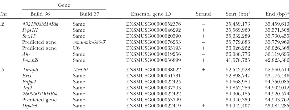
our two QTL were even further reduced from 2.9 to 0.7 Mb and from 4.3 to 0.7 Mb (Figure 1), corresponding to a final reduction in the number of candidate genes from 11 on chromosome 12 and from 43 on chromosome 15 to 7 in each case (Table 1).
Identifying QTGs: Although rigorous experimental testing of all narrowed QTL candidate genes would be ideal, such a strategy is not always practical. Using our narrowed list of seven candidate genes for the chromo-some 12 HDL QTL, here we provide an example of how to arrive at the most probable underlying QTG by judiciously combining publicly available bioinformatics resources with laboratory experiments.
Because trait variation is caused by changes in the function of a protein or by differences in the amount of protein available, we start by searching for SNPs and expression differences between the parental strains of the QTL crosses. For mice, the Mouse Phenome Database (http://phenome.jax.org/phenome) is an excellent resource for comparing SNPs among strains, as it contains SNP locations and annotations from multiple sources with relevant hyperlinks. The Ensembl genome browser (http://www.ensembl.org) is another useful resource for comparing SNPs within transcripts among strains. SNPs found within exons, and in particular annotated nonsynonymous SNPs, should be further investigated to determine whether or not they are situated in functional domains and whether or not the substitutions cause changes in polarity or acidity. This information can also be obtained from sources such as Ensembl or from the Expasy Proteomics Server (http://expasy.org).
TABLE 1
Candidate gene lists from final narrowed QTL
Gene
Chr Build 36 Build 37 Ensembl gene ID Strand Start (bp)a End (bp)a
12 4921508M14Rik Same ENSMUSG00000052376 35,459,173 35,459,613
Prps1l1 Same ENSMUSG00000046292 1 35,569,960 35,571,508
Snx13 Same ENSMUSG00000020590 1 35,632,289 35,730,455
Predicted gene mmu-mir-680-3b ENSMUSG00000076253 35,779,883 35,779,969
Predicted gene U6c ENSMUSG00000065195 1 36,026,262 36,026,368
Ahr Same ENSMUSG00000019256 36,088,776 36,119,695
Immp2l Same ENSMUSG00000056899 1 41,578,735 42,825,386
15 Thrap6 Med30 ENSMUSG00000038622 1 52,542,528 52,560,514
Ext1 Same ENSMUSG00000061731 52,898,747 53,175,446
Enpp2 Same ENSMUSG00000022425 54,668,984 54,750,085
Taf2 Same ENSMUSG00000037343 54,852,286 54,902,012
2600005O03Rik Same ENSMUSG00000022422 54,906,185 54,920,574
Predicted gene Same ENSMUSG00000053749 54,940,359 54,943,762
Depdc6 Same ENSMUSG00000022419 1 54,942,407 55,084,285
Chr, chromosome.
aGenome coordinates are from NCBI Mouse Build 36. bThis gene encodes a microRNA.
For examining gene expression differences, data-bases of expression profiles are increasingly available. In mice, strain-specific mRNA expression profiles of liver tissue for 12 strains are available at http://www. ncbi.nlm.nih.gov/geo (GEO accession GSE10493), and expression QTL data for liver, fat, adipose, and pancreas tissues in up to 33 strains, as well as tissue expression levels in .75 tissue types, are available through the Genomics Institute of the Novartis Foundation (GNF) BioGPS Website and Database (https://biogps.gnf.org). For each candidate gene with available data, an exam-ination of the expression differences among the parental strains should be conducted. In addition, the tissue-specific expression data should be examined if one expects increased expression in a certain tissue type. For example, for our HDL candidate QTGs, we looked for evidence of expression at least two times greater than the median in liver tissue, which plays a critical role in cholesterol metabolism.
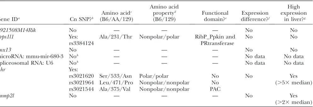
For our seven chromosome 12 candidate genes, we searched these publicly available databases and have compiled the results in Table 2. InPrps1l1andAhr, we found evidence of nonsynonymous SNPs that differ between B6 and 129 and that are the same for the ‘‘high’’ HDL strains NZB and 129. SNP information for RIII and RF is either imputed or not available, so these strains were not included. Prps1l1, a phosphoribosyl-pyrophosphate-synthetase-1-like expressed sequence, has one nonsynonymous SNP. This SNP causes a change
in polarity and is located within the phosphoribosyl transferase domain and the ribose–phosphate pyro-phosphokinase domain; however, it is not currently known whether this substitution causes any change in function.Ahr, the aryl hydrocarbon receptor, has three nonsynonymous SNPs, including one located in a functional domain, the PAC domain, a structurally conserved region involved in the conformational changes that occur in its associated PAS domain during ligand binding and activation for signal transduction (Vreede et al. 2003). Although this alanine-to-valine substitution does not cause a polarity or acidity change, it is known to result in a 4-fold reduction in specific ligand binding (Polandet al.1994). In addition, while we found no significant expression differences . 1.5-fold between 129 and B6 in any of the genes, we did find that bothAhrandImmp2lare highly expressed in liver tissue.Prps1l1, on the other hand, is expressed mainly in the testes.
Bioinformatics has thus reduced a large QTL on chromosome 12 to three possible candidate genes: Prps1l1, Immp2l, and Ahr. With its high expression in liver and a nonsynonymous substitution known to cause a functional change,Ahris the most likely candidate for the chromosome 12 QTL shared by the RIII3129, NZB 3RF, and B63129 crosses.Prps1l1is less likely because, although it has a coding region change that might affect function, it is expressed mostly in testes.Immp2l, on the other hand, has high expression in the liver, but TABLE 2
Chromosome 12 candidate gene evidence summary
Gene IDa Cn SNP?b
Amino acidc
(B6/AA/129)
Amino acid propertyd
(B6/129)
Functional domain?e
Expression difference?f
High expression
in liver?g
4921508M14Rik No — — — No No
Prps1l1 Yes:
rs3384124
Ala/231/Thr Nonpolar/polar RibP_Ppkin and PRtransferase
No No
Snx13 No — — — No No
microRNA: mmu-mir-680-3 Noh — — — No data No data
Spliceosomal RNA: U6 Noh — — — No data No data
Ahr Yes:
Yes (.53median)
rs3021620 Ser/533/Asn Polar/polar No No
rs3021964 Leu/471/Pro Nonpolar/nonpolar No rs3021544 Ala/375/Val Nonpolar/nonpolar PAC
Immp2l No — — — No Yes
(.23median)
a
External gene identification symbol with Ensembl gene identifier number below.
b
Nonsynonymous single nucleotide polymorphism.
c
Amino acid for C57BL/6J and 129S1/SvImJ strains at the protein position number shown (AA no.).
dR-group property of amino acid in C57BL/6J and 129S1/SvImJ strains.
eRibP_Ppkin, ribose-phosphate pyrophosphokinase domain; PRtransferase, phosphoribosyltransferase; PAC, PAS-associated
C-terminal domain.
fmRNA expression difference between 129S1/IvmJ and C57BL/6J strains. gmRNA expression in liver.23median.
unknown expression differences among the strains. The final step in this QTL-to-QTG process is to test these genes in experiments. The expression of Prps1l1 and Immp2lshould be carried out in the relevant strains, and theAhrpolymorphisms should be confirmed. In addi-tion, congenics or knockouts could be tested for predicted differences in their plasma concentrations of HDL. For example, four murine alleles of Ahr are known to exist; one of these alleles, theAhrd
allele from strain DBA/2J, which is shared by strain 129, has been moved as a congenic into the B6 strain. On the basis of high levels of HDL in strain 129 and low levels of HDL in B6, we predict that theAhrd congenic strain will show
increased levels of HDL compared to B6 controls. Hence, these bioinformatics tools not only help narrow QTL to testable lists of candidate genes, but also lead to more focused and hypothesis-driven benchwork.
DISCUSSION
The genetic architecture of complex phenotypes appears to vary considerably from one trait to another, including differences in number of contributing loci, relative magnitude of locus effects, and extent of gene– gene and gene–environment interactions. These factors impact our ability to fully ascertain all genes involved in a quantitative trait (Flintet al. 2005), resulting in an unequal likelihood of success across traits. In addition, poorly understood genetic mechanisms, such as regu-latory enhancers located within unrelated genes, can lead us to the causative sequence variant for a QTL while not leading us to the proper gene (Lettice2002). And inevitably, some QTGs will not satisfy the assumptions of the methods described and will therefore be over-looked. We advocate a conservative approach that in-volves careful scrutiny of chromosomal LOD score plots and allele-effects graphs, since invalid assumptions and methodological imprecision may incorrectly narrow a region, leading to misguided investigations of inappro-priate gene intervals. We also recognize that this gene-centric approach will not always uncover regulatory elements such as undescribed microRNAs that may also be contributing to the observed variation. Regardless, while identifying all genes and regulators that underlie complex traits remains challenging, integrating the methods discussed here will help bridge the gap, in many cases, between finding QTL and identifying candidate QTGs.
Additional resources for reducing candidate QTG lists include tissue expression data (GNF BioGPS Web-site and Database; https://biogps.gnf.org), mRNA expres-sion data from microarrays such as the 12-strain mouse liver microarray survey that we carried out (http:// www.ncbi.nlm.nih.gov/geo, GEO accession GSE10493) and data on gene-specific SNP differences among strains (http://www.jax.org/phenome). Candidate genes can then be tested using a variety of experimental methods,
including RNA interference technology, deficiency complementation tests, knockouts, gene sequencing, pathway analysis, quantitative RT–PCR, Northern blots, Western blots, reporter gene assays, and various other protein assays.
As we have demonstrated, our bioinformatics toolbox can be used to narrow large QTL to a small list of testable candidate genes. Even when only some of the tools can be applied, QTL can still be substantially narrowed. Here, we narrowed our multi-cross QTL on chromosome 12 from 750 genes down to 7 candidates, a reduction of 99.1%, and we narrowed our single-cross QTL on chromosome 15 from 147 genes also down to 7 candidates, a reduction of 95.2%. Which of these individual approaches provides the most narrowing depends on many factors, including the crosses and the chromosomal region involved. As we have shown, it is the integration of these approaches that narrows QTL more than any one method alone. Additionally, we have further demonstrated the power of publicly available data and bioinformatics resources in reducing a testable list of candidate genes down to the most likely candidate gene underlying the mouse chromosome 12 QTL, the aryl hydrocarbon receptor (Ahr).
The authors thank Iaonnis M. Stylianou for phenotyping the 79 strains used in the HAM analysis and Yueming Ding for the megabase positions of the MIT markers and for combining SNP databases from several sources, including resolving markers genotyped differently by multiple groups and sorting out the appropriate DNA strand when necessary. This work was supported by National Institutes of Health grants HL-74086, HL-81162, and HL-77796 to B.P., GM-76468 to Gary Churchill, and the Cancer Core grant to The Jackson Laboratory (CA-34196) from the National Cancer Institute. Support for writing was also provided to S.L.B.H. by the Zoological Society of San Diego’s Center of Conservation and Research for Endangered Species.
LITERATURE CITED
Bogue, M. A., S. C. Grubb, T. P. Maddatuand C. J. Bult, 2007 Mouse
Phenome Database (MPD). Nucleic Acids Res.35:D643–D649. Cervino, A. C. L., A. Darvasi, M. Fallahi, C. C. Mader and
N. F. Tsinoremas, 2007 An integratedin silicogene mapping
strategy in inbred mice. Genetics175:321–333.
Chesler, E. J., S. L. Rodriguez-Zas, J. S. Mogil, J. Usuka, A. Grupe
et al., 2001 In silico mapping of mouse quantitative trait loci. Science294:2423.
Churchill, G. A., and R. W. Doerge, 1994 Empirical threshold
val-ues for quantitative trait mapping. Genetics138:963–971. DiPetrillo, K., X. Wang, I. M. Stylianou and B. Paigen,
2005 Bioinformatics toolbox for narrowing rodent quantitative trait loci. Trends Genet.21:683–691.
Flint, J., W. Valdar, S. Shifmanand R. Mott, 2005 Strategies for
mapping and cloning quantitative trait genes in rodents. Nat. Rev. Genet.6:271–286.
Grupe, A., S. Germer, J. Usuka, D. Aud, J. K. Belknapet al., 2001 In
silicomapping of complex disease-related traits in mice. Science
292:1915–1918.
Gu, L., M. W. Johnsonand A. J. Lusis, 1999 Quantitative trait locus
analysis of plasma lipoprotein levels in an autoimmune mouse model: interactions between lipoprotein metabolism, autoim-mune disease, and atherogenesis. Arterioscler. Thromb. Vasc. Biol.19:442–453.
Hubbard, T. J. P., B. L. Aken, K. Beal, B. Ballester, M. Caccamo
Ishimori, N., R. Li, P. M. Kelmenson, R. Korstanje, K. A. Walsh
et al., 2004 Quantitative trait loci analysis for plasma HDL-cholesterol concentrations and atherosclerosis susceptibility between inbred mouse strains C57BL/6J and 129S1/SvImJ. Arterioscler. Thromb. Vasc. Biol.24:161–166.
Ishimori, N., I. M. Stylianou, R. Korstanje, M. A. Marion, R. Li
et al., 2008 Quantitative trait loci for BMD in an SM/J by NZB/BINJ intercross population and identification of Trps1 as a probable candidate gene. J. Bone Miner. Res.23:1529–1537. Jaiswal, J., J. Ni, I. Yap, D. Ware, W. Spooneret al., 2005 Gramene:
a genomics and genetics resource for rice. Rice Genet. Newsl.22:
9–17.
Jaiswal, P., J. Ni, I. Yap, D. Ware, W. Spooneret al., 2006 Gramene:
a bird’s eye view of cereal genomes. Nucleic Acids Res.34:D717– D723.
Kent, W. J., C. W. Sugnet, T. S. Furey, K. M. Roskin, T. H. Pringle
et al., 2002 The Human Genome Browser at UCSC. Genome Res.12:996–1006.
Khatkar, M. S., P. C. Thomson, I. Tammenand H. W. Raadsma,
2004 Quantitative trait loci mapping in dairy cattle: review and meta-analysis. Genet. Sel. Evol.36:163–190.
Kislev, M. E., A. Hartmannand O. Bar-Yosef, 2006 Early
domes-ticated fig in the Jordan Valley. Science312:1372–1374. Kuhn, R. M., D. Karolchik, A. S. Zweig, H. Trumbower,
D. J. Thomaset al., 2007 The UCSC genome browser database:
update 2007. Nucleic Acids Res.35:D668–D673.
Lettice, L. A., 2002 Disruption of a long-range cis-acting regulator
forShhcauses preaxial polydactyly. Proc. Natl. Acad. Sci. USA99:
7548–7553.
Li, R., M. A. Lyons, H. Wittenburg, B. Paigenand G. A. Churchill,
2005 Combining data from multiple inbred line crosses im-proves the power and resolution of quantitative trait loci map-ping. Genetics169:1699–1709.
Lyons, M. A., R. Korstanje, R. Li, K. A. Walsh, G. A. Churchill
et al., 2004 Genetic contributors to lipoprotein cholesterol lev-els in an intercross of 129S1/SvImJ and RIIIS/J inbred mice. Physiol. Genomics17:114–121.
McClurg, P., M. T. Pletcher, T. Wiltshire and A. I. Sue,
2006 Comparative analysis of haplotype association mapping algorithms. BMC Bioinformatics7:61.
Moore, K. J., and D. L. Nagle, 2000 Complex trait analysis in the
mouse: the strengths, the limitations and the promise yet to come. Annu. Rev. Genet.34:653–686.
Payseur, B. A., and M. Place, 2007 Prospects for association
map-ping in classical inbred mouse strains. Genetics175:1999–2008. Peters, L. L., R. F. Robledo, C. J. Bult, G. A. Churchill, B. J.
Paigenet al., 2007 The mouse as a model for human biology:
a resource guide for complex trait analysis. Nat. Rev. Genet.8:
58–69.
Pletcher, M. T., P. McClurg, S. Batalov, A. I. Su, S. W. Barneset al.,
2004 Use of a dense single nucleotide polymorphism map for
in silicomapping in the mouse. PLoS Biol.2:e393.
Poland, A., D. Palenand E. Glover, 1994 Analysis of the four alleles
of the murine aryl hydrocarbon receptor. Mol. Pharmacol.46:915– 921.
Pringle, H., 1998 Neolithic agriculture: reading the signs of ancient
animal domestication. Science282:1448.
Rollins, J., Y. Chen, B. Paigenand X. Wang, 2006 In search of new
targets for plasma high-density lipoprotein cholesterol levels: promise of human-mouse comparative genomics. Trends Cardio-vasc. Med.16:220–234.
Sen, S., and G. A. Churchill, 2001 A statistical framework for
quan-titative trait mapping. Genetics159:371–387.
Stoll, M., A. E. Kwitek-Black, A. W. Cowley, Jr., E. L. Harris, S. B.
Harrapet al., 2000 New target regions for human hypertension
via comparative genomics. Genome Res.10:473–482.
Sugiyama, F., G. A. Churchill, D. C. Higgins, C. Johns, K. P.
Makaritsiset al., 2001 Concordance of murine quantitative
trait loci for salt-induced hypertension with rat and human loci. Genomics71:70–77.
Szatkiewicz, J. P., G. L. Beane, Y. Ding, L. Hutchins, F. Pardo
-Manuel deVillenaet al., 2008 An imputed genotype resource
for the laboratory mouse. Mamm. Genome19:199–208. Vila, C., P. Savolainen, J. E. Maldonado, I. R. Amorim, J. E. Rice
et al., 1997 Multiple and ancient origins of the domestic dog. Science276:1687–1689.
Vreede, J., M. A.van derHorst, K. J. Hellingwerf, W. Crielaard
and D. M.vanAalten, 2003 PAS Domains. Common structure
and common flexibility. J. Biol. Chem.278:18434–18439. Wang, X., and B. Paigen, 2005 Genetics of variation in HDL
choles-terol in humans and mice. Circ. Res.96:27–42.
Wergedal, J. E., C. L. Ackert-Bicknell, W. G. Beamer, S. Mohan,
D. J. Baylinket al., 2007 Mapping genetic loci that regulate
lipid levels in a NZB/B1NJxRF/J intercross and a combined in-tercross involving NZB/B1NJ, RF/J, MRL/MpJ, and SJL/J mouse strains. J. Lipid Res.48:1724–1734.
Yang, H., T. A. Bell, G. A. Churchilland F. Pardo-Manuel de
Villena, 2007 On the subspecific origin of the laboratory
mouse. Nat. Genet.39:1100–1107.
Zhang, J., K. W. Hunter, M. Gandolph, W. L. Rowe, R. P. Finney
et al., 2005 A high-resolution multistrain haplotype analysis of laboratory mouse genome reveals three distinctive genetic varia-tion patterns. Genome Res.15:241–249.
Zhi-Liang, H., and M. R. James, 2007 Animal QTLdb: beyond a
re-pository. Mamm. Genome18:1–4.