Multiscale Characterization of the Probability Density Functions of Velocity and Temperature Increment Fields.

ABSTRACT

DEMARCO, ADAM WARD. Multiscale Characterization of the Probability Density Functions of Velocity and Temperature Increment Fields. (Under the direction of Dr. Sukanta Basu and Dr. Russell Philbrick.)

The turbulent motions with the atmospheric boundary layer exist over a wide range of spatial and temporal scales and are very difficult to characterize. Thus, to explore the behavior of such complex flow enviroments, it is customary to examine their properties from a statistical perspective. Utilizing the probability density functions of velocity and temperature increments, δu andδT, respectively, this work investigates their multiscale behavior to uncover the unique traits that have yet to be thoroughly studied. Utilizing diverse datasets, including idealized, wind tunnel experiments, atmospheric turbulence field measurements, multi-year ABL tower observations, and mesoscale models simulations, this study reveals remarkable similiarities (and some differences) between the small and larger scale components of the probability density functions increments fields.

©Copyright 2017 by Adam Ward DeMarco

Multiscale Characterization of the Probability Density Functions of Velocity and Temperature Increment Fields

by

Adam Ward DeMarco

A dissertation submitted to the Graduate Faculty of North Carolina State University

in partial fulfillment of the requirements for the Degree of

Doctor of Philosophy

Marine, Earth, and Atmospheric Sciences

Raleigh, North Carolina

2017

APPROVED BY:

Dr. Sukanta Basu

Co-chair of Advisory Committee

Dr. Russell Philbrick Co-chair of Advisory Committee

Dr. Anantha Aiyyer Dr. Steven Fiorino

BIOGRAPHY

ACKNOWLEDGEMENTS

This experience has been quite an exciting adventure! I am very grateful to the U.S. Air Force for providing me with the resources for this wonderful opportunity, but the views expressed in this dissertation are those of the author and do not reflect the official policy or position of the U.S. Air Force, Department of Defense, or the U.S. Government. Without the help from some very influential people, my success during my PhD studies would not have been possible. First, I would like to thank my co-advisor, Dr. Sukanta Basu, for his guidance and involvement in my work. He led me down a path with a clear and coherent vision which was instrumental for my success! In addition, I would like to thank my other co-advisor, Dr. Russell Philbrick. He has had a wealth of experience both in academia and in government and was willing to pass along to me the knowledge he gained, which will continue to guide me as I continue my career as an Air Force officer and scientist.

Also, I would like to thank my other committee members, Dr. Anantha Aiiyer, Dr. Steven Fiorino, and Dr. Yang Zhang for their time and assistance during my research. Many thanks also go out to my fellow group members, Dr. Ping He, Dr. Yao Wang, Dr. Chris Nunalee, and Pat Hawbecker, for being such a great sounding board during this time. They were always willing and able to assist me when I was in bind. Their advice and support was greatly appreciated and needed. Similarly, I am very thankful for the computational resources provided to me by the Air Force Research Laboratory, Department of Defense Supercomputing Resource Center and Dr. Kevin Keefer from the Air Force Institute of Technology. During my studies, I never had to worry if I was going to run out of resources thanks to their support. Additionally, I would be remiss if I did not thank my Air Force leadership, specifically, Lt Col Brian Kabat, for the potential they saw in me and the support they have given me throughout this endeavor. Also, many thanks to my parents for instilling in me the strong work ethic that has carried me throughout my life.

TABLE OF CONTENTS

List of Tables . . . .viii

List of Figures . . . ix

List of Abbreviations . . . .xvii

Chapter 1 Introduction . . . 1

1.1 Motivation . . . 1

1.2 Objectives and Science Questions . . . 5

1.3 Dissertation Outline . . . 6

Chapter 2 Background. . . 9

2.1 Velocity Increment PDFs . . . 11

2.2 Temperature Increment PDFs . . . 14

2.3 Mesoscale Increment PDFs . . . 16

2.4 A Brief Review of Other Statistical Descriptions of Turbulence . . . 18

Chapter 3 Probability Density Functions and Parameter Estimation Techniques 24 3.1 Normal Inverse Gaussian (NIG) . . . 26

3.2 Generalized Hyperbolic Skew Student’s t (GHSST) . . . 29

3.3 Variance Gamma (VG) . . . 32

3.4 Lognormal Superstatistics (LNSS) . . . 33

3.5 Maximum Likelihood Estimation . . . 35

3.6 Extreme Value Theory - Hill Estimator . . . 37

Chapter 4 Estimating Higher-Order Structure Functions from Geophysical Turbulence Time-Series: Confronting the Curse of the Limited Sample Size . . . 39

4.1 Introduction . . . 39

4.2 Limited Sample Size Problem . . . 41

4.3 Quantifying Uncertainty in Structure Function Estimates . . . 42

4.4 Estimatingpmax from Limited Data . . . 45

4.5 Maximum Likelihood-based Structure Function Estimation . . . 48

4.6 Effects of Correlation . . . 51

4.7 Wind Tunnel Data . . . 53

4.8 Alternative Probability Density Functions . . . 55

4.9 Concluding Remarks . . . 56

Chapter 5 Intercomparison of PDFs of Small-Scale Velocity Increments . . . . 58

5.1 Introduction . . . 58

5.2 Description of Data . . . 59

5.4 Probability Density Function Results . . . 61

5.5 Goodness of Fit Techniques . . . 63

5.6 Conclusion . . . 68

Chapter 6 Characterization of Small-Scale Velocity and Temperature Incre-ments in Stably Stratified Boundary Layer Flows . . . 70

6.1 Introduction . . . 70

6.2 Description of Datasets and Methodology . . . 72

6.3 Probability Density Function Models . . . 75

6.4 Stability Impacts on the PDFs . . . 78

6.5 Conclusion . . . 80

Chapter 7 The PDFs of Wind Speed Increments in the Mesoscale Range: Tail Characteristics. . . 82

7.1 Introduction . . . 82

7.2 Description of Observational Data . . . 87

7.2.1 FINO1 . . . 87

7.2.2 Høvsøre . . . 88

7.2.3 Cabauw . . . 88

7.2.4 NWTC . . . 88

7.3 Methodology . . . 89

7.4 Evaluation of the Tail-Index . . . 94

7.5 Probability of Exceedance . . . 104

7.6 Conclusions . . . 106

Chapter 8 The PDFs of Wind Speed Increments in the Mesoscale Range: Model Fitting . . . .109

8.1 Introduction . . . 109

8.2 Mesoscale Probability Density Functions with Model Fit . . . 110

8.3 Quantile-Quantile Plots . . . 113

8.4 Goodness of Fit Evaluation . . . 116

8.5 Diurnal Impacts on Wind Speed Increments . . . 120

8.6 Conclusion . . . 123

Chapter 9 Characterizing the PDFs of Temperature Increments in the Mesoscale Range . . . .125

9.1 Introduction . . . 125

9.2 Probability Density Functions of Mesoscale Temperature Increments . . . 127

9.3 Quantile-Quantile Plots and Goodness of Fit Test . . . 129

9.4 Diurnal Impacts on Temperature Increments . . . 133

9.5 Conclusion . . . 136

Chapter 10 PDFs of Simulated Wind Speed and Temperature Increment Series138 10.1 Introduction . . . 138

10.3 Model Configuration . . . 142

10.4 Wind Speed and Temperature Probability Density Functions from WRF . . . 144

10.5 Statistical Evaluation of the Probability Density Functions . . . 149

10.6 Diurnal Variations in Wind Speed and Temperature Increments in WRF . . . 156

10.7 Conclusion . . . 159

Chapter 11 Conclusions and Future Directions . . . .163

11.1 Summary of Work . . . 163

11.2 Future Directions . . . 167

References. . . .171

Appendix . . . .187

Appendix A Computational Codes . . . 188

A.1 Normal Inverse Gaussian Distribution (NIG) . . . 188

A.2 Generalized Hyperbolic Skewed Student t’s Distribution (GHSST) . . . 193

A.3 Variance Gamma (VG) . . . 195

A.4 Lognormal Superstatistics (LNSS) . . . 198

A.5 Hill Estimator . . . 198

A.6 Probability of Exceedance . . . 199

LIST OF TABLES

Table 4.1 Tail-index (γ∗) and maximum moment order (pmax) for NIG distributed variates of varying sample sizes and with three different parameter

combi-nations. . . 46

Table 5.1 Mean flow characteristics of the measurements.U is the mean velocity,σu is the standard deviation,Ti and Li represent the characteristic time and length scale, respectively and f is the data sampling frequency. . . 60

Table 5.2 Goodness of Fit Test for SLTEST data, corresponding to Figure 5.2 for three select separations . . . 66

Table 5.3 Goodness of Fit Test for ONERA data, corresponding to Figure 5.3 for three select separations . . . 67

Table 6.1 Number of samples in each stability class . . . 74

Table 7.1 Description of measurement sites . . . 87

Table 7.2 Exceedance Probability (%) for right tail (τ = 10 min) . . . 106

Table 7.3 Exceedance Probability (%) for right tail (τ = 60 min) . . . 107

Table 8.1 A2 LandA2Rstatistics for the mesoscale wind speed increments the four sites atτ = 10 min, 60 min, and 360 min. The results are the median, minimum, and maximum height values for the NIG and GHSST models. See Eq. 8.1. 119 Table 9.1 A2_LandA2_Rstatistics for the mesoscale temperature increments for the four sites at τ = 10 min, 60 min, and 360 min. The results are the median, minimum and maximum height averaged values for the NIG and GHSST models. See Eq. 8.1. . . 131

Table 10.1 The median two sample Anderson-Darling test (A2_nm) results comparing the various WRF model wind speed increment distributions against the observed pdfs for 2012 for d02 (9 km). . . 155

Table 10.2 Same as Table 10.1 exceptA2_nm for temperature increments . . . 156

Table 10.3 RMSE summed over the range of separation as depicted in Figure 10.11 comparing theαvalues obtained from wind speed observations against the seven different PBL schemes. . . 159

LIST OF FIGURES

Figure 1.1 Atmospheric normalized velocity increment pdf at (τ = 4 s) overlaid with a Gaussian distribution as indicated with the solid line (adapted from [48]). 3 Figure 1.2 a) United States Air Force (USAF) laser-guided telescope in Albuquerque,

New Mexico [168], b) Blurred image of a satellite obtained from the tele-scope indicative of turbulence impacts [168]. . . 5

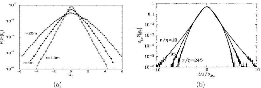
Figure 2.1 a) An example of non-normalized surface wind velocities increment (ur) pdfs from an atmospheric dataset collected in Denmark. The spatial scales (r) range from 1.3 m to 20 m (adapted from Ragwitz and Kantz (2001, [214]), Figure 4). b) The transition of normalize velocity increments (∆u/σ∆u) from small (r/η = 10) to large (r/η = 245) scales. Here, the separation distance r is being normalized by η, the Kolmogorov length scale, η = (ν3/)1/4, where ν is the viscosity of the fluid (adapted from Herweijer (1995, [108]) Figure 5.1). . . 12 Figure 2.2 Similar examples as Figure 2.1, but for small scale temperature a) adapted

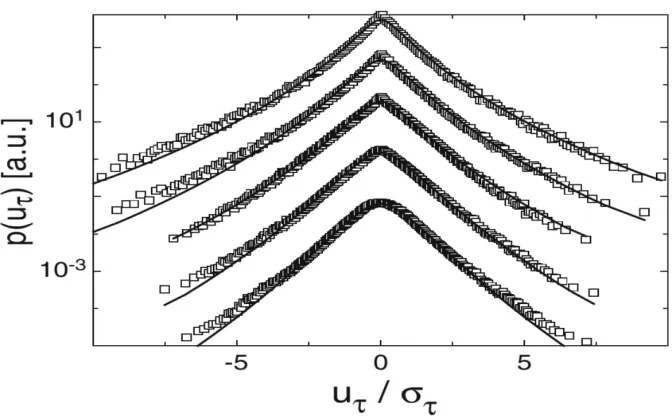
from Ching (1991,[63]). b) adapted from Warhaft (2000, [269]). . . 14 Figure 2.3 This example shows the evolution of the velocity increment pdf for larger

scale motions from 2.5, 25, 250, and 4,000 sec, from top-bottom respec-tively. The solid lines represent the log-normal model (adapted from [49]). 17 Figure 2.4 a) Depiction of small-scale turbulent energy cascade (adapted from

An-drews and Philips (2005, [10])). Based on K41 theory, the inertial range in fully-developed turbulence is bounded by a region of eddies sizes between the outer (L0) and inner length scale (l0). b) Example of “2/3” scaling

law within a turbulent random field (adapted from Wittwer (2013, [272])). 19 Figure 2.5 a) Exponent ζp vs.p. Inverted white triangles: data from Van Atta and

Park (1972) [258]; black circles, white squares and black triangles: data from Anselmetet al.(1984) with increasingRe: + signs: wind tunnel data using ESS; straight dash-dot line fromζp =p/3 (K41). The model fit lines are from the various cascade models. (adapted from [94]), b) The scaling exponents (ξn) for the scalar increments (∆θr) with the separation dis-tance in the inertial range. Squares are experimental results from Antonia

et al.(1984, [14]), with vertical bars showing the uncertainty in the data. Circles and diamonds are from Meneveau et al. (1990, [173]. The dashed lines are estimates of the uncertainty (adapted from [238]). . . 21 Figure 2.6 a) Third order SF of velocity increments versus spatial separation (not

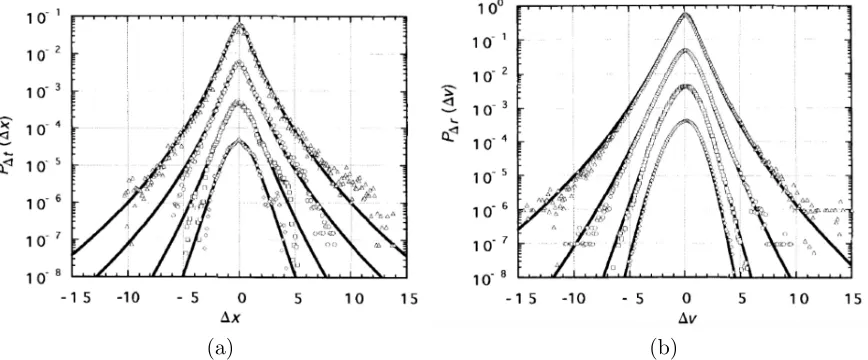
Figure 3.1 a) The stock market price changes (∆x) for different τ=640 sec, 5,120 sec, 40,960 sec, and 163,804 sec (from top to bottom) . b) turbulence flow (∆v) for different separations (δr = 3.3η, 18.5η, 138η, and 325η) from small to large scale, situated from top to bottom, respectively, (adapted from [101]). . . 25 Figure 3.2 An illustration of a daily IBM-stock returns fitted with generalized

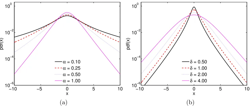
hy-perbolic, hyperbolic and Gaussian distributions (adapted from [42]). . . . 26 Figure 3.3 NIG pdfs for different values ofα (left panel) and δ (right panel). For all

the pdfs, µand β are assumed to be equal to zero. For the left figure,δ is kept constant at 2. In the right figure, α is taken as 4. . . 28 Figure 3.4 GHSST pdfs for different values ofν (left panel) andδ (right panel). For

all the pdfs,µassumed to be equal to zero andβ ∼0. For the left figure, δ is kept constant at 2. In the right figure,ν is taken as 4. . . 30 Figure 3.5 VG pdfs for different values of α (left panel) and λ(right panel). For all

the pdfs,µandβ assumed to be∼0. For the left figure,λis kept constant at 1. In the right figure, α is taken as 1. . . 32 Figure 3.6 LNSS pdfs for different values of µ (left panel) and s (right panel). For

the left figure, sis kept constant at 1. In the right figure, µis taken as 1. 34 Figure 3.7 Example of a Hill plot for the transmission times of web files. The

asymp-totic value occurs atα∼1, signifying a Pareto-type distribution (adapted from Crovella et al. (1998, [71])). . . 38

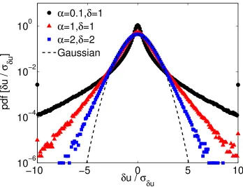
Figure 4.1 NIG distributed variates with three different parameter combinations: (a) α = 0.1, δ = 1, (b) α = 1, δ = 1, and (c) α = 2, δ = 2. For all these cases, the parameters µand β are assumed to be equal to zero. For each case, 107 samples were generated using Rydberg’s algorithm [216]. The distributions were normalized by the standard deviationσδu. A Gaussian pdf is overlaid (dashed line) as a reference. . . 43 Figure 4.2 “Empirical” S6 box plots for three different NIG distributions with

pa-rameter combinations: (a) α = 0.1, δ = 1, (b) α = 1, δ = 1, and (c) α = 2, δ = 2. The parametersµ and β are assumed to be equal to zero. The sample sizes (N) are varied from 103to 107. One hundred realizations are used for the construction of the box plots. The dashed magenta lines represent the true S6 values based on Eq. 4.1. . . 44

Figure 4.3 Rank-order (a.k.a. Zipf) plots for NIG distributed variates with three different parameter combinations: (a) α = 0.1, δ = 1, (b) α = 1, δ = 1, and (c) α = 2, δ = 2. The parameters µ and β are assumed to be equal to zero. The sample sizes (N) are varied from 104 to 107. The tail-indices (γ∗) are estimated for N = 104 (dot-dashed) and N = 107 (dashed) and reported in the bottom-left corner of the plots. . . 46 Figure 4.4 Hill plots for NIG distributed variates with three different parameter

Figure 4.5 Box plots of K-S test statistic (D) comparing MME (left panel) versus MLE (right panel) results. The following parameters are utilized to gener-ate the random varigener-ates: α= 0.1,β= 0,µ= 0, andδ = 1 (heavy-tailed). The sample sizes (N) are varied from 103 to 106. As before, 100 realiza-tions are used for the construction of the box plots. . . 50 Figure 4.6 MLE-basedS6box plots for three NIG distributions with parameter

com-binations: (a) α= 0.1, δ= 1, (b)α= 1, δ= 1, and (c) α= 2, δ= 2. The parameters µ and β are assumed to be equal to zero. The sample sizes (N) are varied from 103 to 106. One hundred realizations are used for the construction of the box plots. The dashed magenta lines represent the true S6 values based on Eq. 4.1. . . 51

Figure 4.7 Realizations of i.i.d (top panel) and correlated (bottom panel) NIG vari-ates. Both realizations follow the same NIG distribution with prescribed parameters: α=1, β = 0,µ= 0, andδ=1. . . 52 Figure 4.8 “Empirical” (top panel) and MLE-based (bottom panel) S6 box plots for

correlated NIG variates. The following parameters are utilized to generate the random variates: α = 1, β = 0, µ = 0, and δ = 1. The sample sizes (N) are varied from 103 to 106. One hundred realizations are used for the construction of the box plots. The dashed magenta lines represent the true S6 value based on Eq. 4.1. . . 53

Figure 4.9 Analyses of ONERA S1 wind tunnel data. Selected increment: r = 8.2 mm or τ = 4 ×10−4 sec, (a) corresponding PDF with NIG-MLE fit, (b) “Empirical” S6 box plots, (c) NIG-MLE S6 box plots. One hundred

realizations are used for the construction of the box plots. The dashed magenta line represent the S6 values based on Eq. 2.2 using the entire

data set. The dot-dashed lines represent an uncertainty of±10% around the magenta line. . . 54 Figure 4.10 Same a Figure 4.9, except forr= 277.8 mm or τ = 1.35×10−2 sec. . . . 55 Figure 4.11 Top panel: comparison of fitted NIG and LNSS pdfs for i.i.d NIG variates.

The sample size is 106_{. Bottom panel: MLE-based S}

6 box plot for i.i.d.

NIG variates with the (incorrect) assumption of LNSS as the underlying pdf. Due to high computational costs associated with numerical integra-tion of the LNSS pdf, the sample sizes (N) are only limited to 104 _{in this}

Figure 5.1 Second-order structure function (S2) as a function of normalized

spa-tial separation (r/Li) from turbulence series a) SLTEST [141] and b) ONERA-Modane S1 wind tunnel [97]. The insets depict the correspond-ing local slopes (ζ2 = d(log(S2)/d(log(r/Li)) from S2 with the dashed

line representing the expected IR scaling exponent, ζ2 ∼ 0.70. The

scal-ing exponent can be reliably estimated within the vertical dotted lines. The red dots were selected to represent three distinctly different regimes within the turbulence signal. . . 61 Figure 5.2 The pdfs of normalized velocity increments (δu/σδu) corresponding to

r/Li = 3.5×10−4, r/Li = 3.5×10−3, and r/Li = 5.4×10−2 are shown in the left, middle, and right panels, respectively for the SLTEST at-mospheric data. The equivalent τ values are shown in the legend. The empirical pdfs are then fitted using MLE with the four distributions de-scribed in Chapter 3. The dashed line in all figures designate the Gaussian distribution for reference. . . 62 Figure 5.3 The pdfs of normalized velocity increments (δu/σδu) corresponding to

r/Li = 2.0×10−3, r/Li = 3.0×10−2, and r/Li = 5.1×10−1 are shown in the left, middle, and right panels, respectively for the ONERA wind tunnel data. The equivalentτ values are shown in the legend. The empir-ical pdfs are then fitted using MLE with the four distributions described in Chapter 3. The dashed line in all figures designate the Gaussian dis-tribution for reference. . . 63 Figure 5.4 a) K-S statistic using histogram binning (Dbin) of ONERA data compared

against the various pdf models as a function ofr/Lion a log-linear plot. b) Depicts a linear-linear representation of Figure 5.3b) zoomed into the core of the distribution. c) K-S evaluation using various binning techniques (described in itemized list above) for the ONERA turbulence dataset comparing the NIG distribution as a function of separation r/Li on a log-log plot. The black symbols in (a) correspond to the blue curve in (c). 64 Figure 5.5 K-S plots based on edf (Dedf) for the different distribution as a function

of normalized separation distance (r/Li) for SLTEST (a) and ONERA (b). For these computations, the velocity increments are not normalized. The inertial-range scaling exponents can be reliably estimated within the vertical dotted lines (SLTEST) and vertical dashed lines (ONERA). . . . 67 Figure 5.6 Dependence of the NIG pdf parameters on the normalized separating

distance (r/Li) for SLTEST (red-solid line) and ONERA (blue-dashed line). For these computations, the velocity increments are not normalized. The inertial-range scaling exponents can be reliably estimated within the vertical dotted lines (SLTEST) and vertical dashed lines (ONERA). . . . 69

Figure 6.2 Median velocity increment pdfs for four different stability classes using Ohya wind-tunnel data: a) S1, 0 < ζ ≤ 0.25; b) S2, 0.25 < ζ ≤ 0.50; c) S3, 0.50 < ζ ≤ 1.0; and d) S4, ζ >1.0. . . 76 Figure 6.3 Same as Figure 6.2 except the median temperature increment pdf. . . 77 Figure 6.4 Temperature ramp-cliff features from a) Sreenivasan (1979, [239]) b)

Time-series segment taken from the S1 stability class at the 0.16 m sensor height from Ohya’s dataset. . . 78 Figure 6.5 Median values of NIG parameters a) α and b)β as a function ofτ from

the velocity datasets from Ohya (2001, [200]) based on the four different stability classes: S1, (0< ζ ≤0.25); S2, (0.25< ζ ≤0.50); S3, (0.50< ζ ≤

1.0); and S4, (ζ >1.0). . . 79 Figure 6.6 Same as Figure 6.5, except for the temperature dataset. . . 80

Figure 7.1 Probability density functions of wind speed increments for FINO1 (a-c), Høvsøre (d-f), Cabauw (g-i), and NWTC (j-l) for the three sets ofτ values from 10 min, 60 min and 360 min. . . 86 Figure 7.2 a) FINO1 (100 m) 2004–2012, b) Høvsøre (116.5 m) 2005–2015, c) Cabauw

(200 m) 2001–2015, d) NWTC (M2; 80 m) 2004–2014 . . . 89 Figure 7.3 a) Rank-order (a.k.a. Zipf) plots for generalized Pareto distributed

vari-ates with three different c values. The parameters a and b are assumed to be equal to 1 and 0, respectively. b) The estimated γH values for these cases. It is clear that γH ≈1/c fork >1000. . . 90 Figure 7.4 A realization of the GHSST variates (sample size = 107) is generated

using the following parameters: ν = 6, β = 0.5, µ =−0.125, and δ = 1. A subset of these variates is shown in (a) as an illustrative example. The mean of the variates is depicted by the dashed red line. The green lines denote three times the standard deviation around the mean. The analytical (black line; [2]) and sample (magenta circles) pdfs are shown in (b). For comparison, a Gaussian pdf (dot-dashed line) with zero mean and unit variance is overlaid on this panel. The tails of the GHSST and Gaussian pdfs are shown (c). Since the right and the left tails of the GHSST pdf behave differently, they are shown separately. Clearly, the right tail exhibits a linear behavior in this log-log representation. Rank-order (a.k.a. Zipf) plots for the GHSST and Gaussian distributed variates are shown in (d). Estimated tail indices (γH) utilizing the Hill plot are documented in (e). . . 92 Figure 7.5 Sensitivity of estimated γH values with respect to sample size. All the

GHSST variates are generated using the same parameters as in Figure 7.5. (a) and (b) correspond to the left and right tails, respectively. . . 94 Figure 7.6 Complementary cumulative distribution function (F_{) from the NWTC1min}

Figure 7.7 _{The Hill plots for wind ramp distributions based on the NWTC1min} time-series. The red (solid) and blue (dashed) lines represent ramp-up (δu+) and ramp-down (δu−) cases, respectively. (a) - (d) correspond to the following scenarios, respectively: (i) τ= 10 min,z= 80 m; (ii) τ= 60 min,z= 80 m; (iii)τ= 180 min, z= 80 m; and (iv)τ= 180 min,z= 10 m. 96 Figure 7.8 The Hill plots for wind ramp distributions based on the subsets of

1-min-average NWTC wind speed time-series. Each subset contains contiguous 578 thousand samples. A total of one hundred randomly selected subsets are utilized for these plots. The top, middle, and bottom panels represent τ = 10 min, 60 min, and 180 min, respectively. Ramp-up and ramp-down results are shown in left and right panels, respectively. The solid lines, dark shaded areas, and the light shaded areas correspond to the medians, 25th-75th percentile ranges, and 10th-90th percentile ranges, respectively. 98 Figure 7.9 The Hill plots of wind ramp distributions from four field sites: FINO1

((a); sensor height: 100 m), Høvsøre ((b); sensor height: 116 m), Cabauw ((c); sensor height: 200 m), NWTC ((d); sensor height: 80 m). For all the cases, 10-min-averaged wind speed are utilized. The time increment (τ) is 10 min. The ramp-up (δu+) and ramp-down (δu−) statistics are denoted by red (solid) and blue (dashed) lines, respectively. . . 100 Figure 7.10 Same as Figure 7.9, except for time increment (τ) of 60 min. . . 101 Figure 7.11 Same as Figure 7.9, except for time increment (τ) of 180 min. . . 102 Figure 7.12 The averaged values of tail indices (hγHi) as a function time-increment

(τ). Wind ramp-up data from all the available sensors from all the four sites are utilized here. . . 103 Figure 7.13 Same as Figure 7.12, except for ramp-down events. . . 104

Figure 8.1 10-min wind speed increment pdfs for the following locations and tower heights in order of complexity from smooth ocean surface to complex terrain. a) FINO1-100 m; b) Høvsøre-100 m; c) Cabauw-80 m; d) NWTC-80 m. Overlaid on each figure are the estimation model pdfs using MLE for NIG, VG, and GHSST and MME for LNSS. The dashed black line represents the Gaussian distribution. . . 112 Figure 8.2 Same as Figure 8.1 except for the 360-min wind speed increment pdf. . . 113 Figure 8.3 Q-Q plots comparing wind speed increments against the estimated NIG

model distributions for three different τ (10 min, 60 min, and 360 min) and four locations (FINO1, Høvsøre, Cabauw, and NWTC). The corre-sponding K-S and A-D test statistics are depicted in the legend. . . 114 Figure 8.4 Q-Q plots comparing wind speed increments against the estimated GHSST

model distributions for three different τ (10 min, 60 min, and 360 min) and four locations (FINO1, Høvsøre, Cabauw, and NWTC). . . 115 Figure 8.5 Edf-based K-S (D) box plots for the wind speed time series increments

Figure 8.6 NIG parameter (α) for full series of wind speed increments as a function of τ for a) FINO1, b) Høvsøre, c) Cabauw, and d) NWTC for different heights. . . 121 Figure 8.7 NIG parameter (α) for day (left column) and night (right column) series of

wind speed increments as a function of τ for a)-b) FINO1, c)-d) Høvsøre, e)-f) Cabauw, and g)-h) NWTC for different heights. . . 122

Figure 9.1 Probability density functions for mesoscale temperature increments across various geographical locations and a range of temporal separation τ. (a-c) Høvsøre, (d-f) Cabauw, (g-i) NWTC. Overlaid on each figure are the heights of the temperature measurements . . . 128 Figure 9.2 τ = 180 min. a) Høvsøre-100 m; b) Cabauw-80 m; c) NWTC-80 m . . . . 129 Figure 9.3 Q-Q plots comparing temperature increments against the estimated NIG

model distributions for three different τ (10 min, 60 min, and 360 min) and three locations (Høvsøre (100 m), Cabauw (80 m), and NWTC (80 m)). . . 132 Figure 9.4 Same as Figure 9.3 except the comparison between observed temperature

increment and GHSST. . . 133 Figure 9.5 NIG parameter (α) for full series of temperature increments as a function

of τ for a) Høvsøre, b) Cabauw, and c) NWTC for different heights. . . . 135 Figure 9.6 NIG parameter (α) for day (left column) and night (right column) series

of temperature increments as a function of τ for a)-b) Høvsøre, c)-d) Cabauw, and e)-f) NWTC for different heights. . . 136

Figure 10.1 Examples of mesoscale model-based synthetic wind speed increments from a) The National Institute of Water and Atmospheric Research (NIWA) in New Zealand [255] and b) The National Renewable Energy Laboratory’s (NREL) Wind Integration National Dataset (WIND) Toolkit (WTK) over the continental United States [80]. . . 140 Figure 10.2 a) WRF domain configuration. The circles represent the approximate

lo-cations of the simulated towers at Høvsøre ( ), FINO1 ( ), and Cabauw ( ). b) Model’s vertical grid resolution versus height in AGL (km). The inset depicts the 10 lowest vertical grid points which are considered in this study. . . 143 Figure 10.3 Pdf of wind speed increments comparing observations and WRF results

Figure 10.5 Wind speed increment pdf at τ = 10 min, a) Cabauw 1-year observa-tions and 1-year d03 modeling results for the simulated tower identical to Figure 10.3c), b) Cabauw 14-year observations and 1-year d03 modeling results for the simulated tower. These two figure produce nearly iden-tical K-S results between the two comparing the PBL schemes and the observations. . . 148 Figure 10.6 Different widths to showcase the sensitivity to the choice of pdf

bin-ning. The following is the dynamic range (maximum and minimum) and bin-widths for the figures above: a) ±12 and 0.5 width, b) ±12 and 0.1, c) ±15 and 0.25. . . 149 Figure 10.7 Boxplots ofDnm for d02 for a) 10 min, b) 60 min, and c) 360 min

incre-ments. The set of box plots represent different locations for each of the seven PBL schemes (x-axis). . . 151 Figure 10.8 Same as Figure 10.7 exceptDnm results for d03. . . 152 Figure 10.9 Same as Figure 10.7 exceptDnm results for temperature increments for

only Høvsøre and Cabauw towers. . . 153 Figure 10.10Same as Figure 10.9 except theDnm results for d03 . . . 154 Figure 10.11NIG parameter (α) for day (left column) and night (right column)

se-ries of wind speed increments as a function of τ comparing seven PBL schemes against model estimated α values for (a-d) Cabauw and (e-f) FINO1 for different heights for the d02 (a,b,e,f) and d03 (c,d,g,h) do-mains. The observational data is computed using bootstrap method with 100 randomized samples. The dashed black lines, dark grey shaded areas, and the light grey areas correspond to the medians, 25th-75th percentile ranges, and 10th-90th percentile ranges, respectively. . . 161 Figure 10.12Same as Figure 10.11 except for Temperature increments for (a-d) Cabauw

and (e-f) Høvsøre for different heights the d02 (a,b,e,f) and d03 (c,d,g,h) domains. . . 162

List of Abbreviations

ABL . . . Atmospheric Boundary Layer

A-D . . . Anderson Darling

DoD . . . Department of Defense

cdf . . . Cumulative Distribution Function

edf . . . Empirical Distribution Function

ESS . . . Extended Self-Similarity

EV . . . Extreme value

GHSST . . . Generalized Hyperbolic Skew Student’s t

GoF . . . Goodness of Fit

IR . . . Inertial Range

i.i.d. . . Independent and identically distributed

KH . . . Kelvin-Helmholtz

K-S . . . Kolmogorov-Smirnov

LNSS . . . Lognormal Superstatistics

MLE . . . Maximum Likelihood Estimation

MME . . . Method of Moments Estimation

NIG . . . Normal Inverse Gaussian

NWP . . . Numerical Weather Prediction

pdf . . . Probability Density Function

Q-Q . . . Quantile-Quantile

RE . . . Reynolds number

SF . . . Structure Function

TKE . . . Turbulent kinetic energy

USAF . . . United States Air Force

VG . . . Variance Gamma

Chapter 1

Introduction

Could I just look at something which everybody had been looking at for a long time and find something dramatically new?

Benoit Mandelbrot (2010)

1.1

Motivation

The Earth’s atmosphere is highly complex with motions spanning across a wide range of spatio-temporal scales, from the large globally driven circulations to the small-scale turbulent eddies. The size of these features range from thousands of kilometers to on the order of millimeters and can occur over a range of weeks to seconds [245]. This extensive range leads to an exorbitant number of degrees of freedom, making it nearly impossible to accurately predict the changes in the flow over these scales.

first principles (i.e., the Navier-Stokes equations) due to the inability to have a closed-form solution. In fact, this issue has been coined, by many, as one of the most important unsolved problems in modern physics [253]. Thus, in the field of fluid dynamics, it is quite customary to describe the turbulent characteristics with the use of statistics in order to identify similarities and differences between various flow types (e.g, Reynolds number, boundary conditions, large-scale forcing, etc.). Another area of turbulence research focuses on identifying the dynamical structures of turbulence (e.g., vortex elements [147, 194]). Though, for this work, the primary method of evaluation is geared towards expanding on the former point of view. In fact, in a highly regarded fundamental turbulence book, Monin and Yaglom (1971, [179]) stated:

“The theory of turbulence by its very nature cannot be other than statistical, i.e. an individual description of the fields of velocity, pressure, temperature, and other characteristics of turbulent flow is in principle impossible. Moreover, such description would not be useful even if possible, since the extremely complicated and irregular nature of all the fields eliminates the possibility of using exact values of them in any practical problems...”

Utilizing the techniques and theories addressed Monin and Yaglom’s book, countless efforts, some of which will be addressed in detail in Chapter 2, were made to identify statistical prop-erties of various turbulent flows. From an experimental perspective, a number of works strive to uncover statistical scaling properties and universal behavior. At the heart of this work is the 1-D velocity (or temperature) increment series,δu (or δT):

δu(r) =u(x+r)−u(x), (1.1)

whereris the spatial separation (similarlyτ represents temporal separation). It has been shown that the probability density functions (pdfs) of both velocity and temperature increments, across a wide spectrum of scales, have very unique and self-similar properties [184, 251, 257], which are quite different from classical turbulence theory [137].

In many applications, it is customary to assume a Gaussian (or normal) distribution for random continuous processes. However, from the pdf perspective it becomes clear that there are distinct differences between what is observed and the normal distribution. For instance, the tails of the pdf are much heavier (i.e., more extended) for the observed data, indicating that extreme wind events (i.e., strong wind increments) have a much higher probability of occurrence compared to the assumed Gaussian distribution (see black arrow). Predicting this deviation is of great importance to a number of application, in particular the wind energy industry. Therefore, it is important to gain a comprehensive understanding into these features over a range of various time and space scales given the extreme difference observed in Figure 1.1.

Figure 1.1: Atmospheric normalized velocity increment pdf at (τ = 4 s) overlaid with a Gaus-sian distribution as indicated with the solid line (adapted from [48]).

model. A few studies have shown the ability of pdf models to capture the traits of velocity and temperature increments (e.g., log-normal [56] and stretched-exponential [63]) from a visual perspective. However, to the best of our knowledge no study has attempted to provide a quan-titative analysis into the quality of the fits, especially across a wide range of scales. Therefore, this work is devoted to filling that void. Furthermore, examination of multi-year wind and tem-perature datasets provides a unique opportunity to explore the long-term statistical behavior of these fields. Unfortunately, these extensive datasets have not been utilized in the past for this type of evaluation, thus this work will be the first to reveal the atmospheric boundary layer (ABL) characteristics of the wind speed and temperature increment pdfs using such long-term data. Having the ability to properly characterize and estimate these increments can be of great benefit to a number of practical applications.

From a military perspective, for example, the Department of Defense (DoD) has become increasingly interested in understanding and predicting the effects small-scale atmospheric tur-bulence has on optical wave propagation in order to minimize the impacts on various DoD space and airborne surveillance applications (see Figure 1.2). The influences of turbulence can have direct effects on the propagation of light and sound waves in the atmosphere. For instance, a phenomenon called scintillation, which is the fluctuation of the beam intensity, is due almost exclusively to atmospheric temperature variations [151, 207]. Additionally, outside of the small scale range, the larger scale influences are still not well-defined [10], thus work is still being conducted to further enhance our understanding of the turbulent nature of our very complex atmosphere. Further, the larger scales often describe the sources and character of small scales, because of the way they are linked. The energy of the large scales provides the driving force for small scales, and the rates of turbulent dissipation determines the lifetime of large scales. There-fore, with a proper characterization of velocity and temperature increments, improvements can be made in this arena. As eloquently stated by Lawrence and Strohben (1970, [151]):

for optical effects. We shall see that the small-scale fluctuations are primarily re-sponsible for intensity scintillation effects, and the large-scale fluctuations produce optical phase effects. A Gaussian model having too few adjustable parameters ties these together in an arbitrary and unrealistic way and engenders misleading and erroneous predictions.”

(a) (b)

Figure 1.2: a) United States Air Force (USAF) laser-guided telescope in Albuquerque, New Mexico [168], b) Blurred image of a satellite obtained from the telescope indicative of turbulence impacts [168].

Furthermore, proper characterization of the velocity and temperature increments and iden-tifying a suitable pdf model can aid in the testing and validation of numerical weather predic-tion (NWP) models. For instance, convenpredic-tional validapredic-tion methods generally utilize tradipredic-tional statistical methods, such as root mean square error and correlation coefficient to compare ob-servations against model results [123]. However, these techniques do not provide a rigorous evaluation. From this standpoint, the characterization of the observed atmospheric pdf incre-ments can be used as a surrogate for providing a benchmark for future model development.

1.2

Objectives and Science Questions

observational and modeling datasets are used to explore the boundary layer characteristics of wind and temperature increments. With the use Goodness of Fit (GoF) techniques, an examination into the model pdfs is conducted to identify a suitable model for practical use. Therefore, the primary science questions raised by this research are:

1) Do velocity and temperature have a universal behavior across a range of spatio-temporal scales? This science question will be addressed in Chapters 5, 6, 7, 8, 9, and 10.

2) If so, can we identify a universal probability density function (pdf) model which can be used for both velocity and temperature increments? This science question will be addressed in Chapters 5, 6, 7, 8, 9, and 10.

3) Do various stability conditions influence the behavior of the pdf fields? If so, do the pdf models still capture these traits? This science question will be addressed in Chapters 6, 8, 9, and 10.

4) How well do the state-of-the-art mesoscale models capture the observed pdfs of wind and temperature increments? This science question will be addressed in Chapter 10.

1.3

Dissertation Outline

The overarching theme of this research is to use a myriad of long-term, research-grade datasets to identify the similarities and differences in the wind and temperature pdfs from different scales of motion. Therefore, the chapters of this dissertation are organized as follows:

• Chapter 2 provides a brief background into the pdf concepts and brief literature review of the current state and understanding of the increment pdfs.

discussion on the maximum likelihood estimation technique which was employed throughout this work.

• Chapter 4 discusses some of the current inherent shortfalls in moment estimation that exist in terms of the limited sample size that are prevalent in typical geophysical datasets. This study showcases the performance of a model pdf, Normal Inverse Gaussian (NIG), and the ability to estimate it using the maximum likelihood estimation technique. This type of analysis was never considered for turbulence data. The material presented in this chapter is published as the following publication: DeMarco, A.W. and Basu, S. (2017) “Estimating Higher-Order Structure Functions from Geophysical Turbulence Time-Series: Confronting the Curse of the Limited Sample Size”, Physical Review E, Volume 95, page 052114.

• Chapter 5 examines high-Reynolds number flows from laboratory and atmospheric boundary layer settings to explore the model pdfs fits to determine how well each model can represent the small-scale turbulence data.

• In Chapter 6, using a state-of-the-art, stably stratified wind tunnel dataset, we explore the variability in pdf parameters as a function of stability.

• Chapter 7 focuses specifically on the tails of the mesoscale range wind distributions with emphasis on the extreme ramp-up and ramp-down characteristics. This work is specifically beneficial to the wind energy industry for predictive purposes. A portion of this material presented in this chapter is in peer-review as the following publication: DeMarco, A.W. and Basu, S. (2017) On the Tails of the Wind Ramp Distributions, Wind Energy.

• Utilizing the dataset from the previous chapter, Chapter 8 tests the different pdf models against each other using GoF techniques (i.e., Kolmogorov-Smirnov and Anderson-Darling tests) to determine which model is able to fit the data the best. We also document the effects of atmospheric diurnal conditions on the pdf parameters.

examination.

• A state-of-the-art mesoscale model, Weather Research and Forecasting (WRF) is evaluated in Chapter 10 to see how well a handful of planetary boundary layer schemes are able to capture the pdf behavior in both wind and temperature increments.

• In Chapter 11, a conclusion of the work along with future directions is summarized.

Chapter 2

Background

The study of turbulence is rooted in the understanding and characterization of the statistical properties of the flow. From this point of view, the probability density functions (pdfs) of two-point difference (or increments, see Eq. 1.1) of these stochastic variables can shed light into unique features. The reasons for increased interest and an ability to accurately estimate the pdfs of these flows is that it can uncover all the statistical moments (mean, variance, etc.) of the turbulence field. Moreover, the tails of the distribution can provide great insight into predicting extreme events [251]. Thus, evaluating and determining an estimation of turbulence can be beneficial to a number of fields, as addressed in Chapter 1.

By definition, thepth order moment of a variablexabout the origin (x= 0) can be computed as an integral over the pdf of the velocity or temperature increment:

hxpi=

Z ∞

−∞

xpf(x)dx, (2.1)

pdfs of these increments possess important information which can easily be lost using the SF approach, as it only computes the moments of the increments. Therefore, increment pdfs are a necessary tool to evaluate the distinct properties of stochastic variables, such as intermittency. Sreenivasan (1999, [236]) defines turbulence as intermittent and having a non-Gaussianity appearance: “Roughly speaking, intermittency means that extreme events are far more prob-able than can be expected from Gaussian statistics and that the probability density functions (pdfs) of increasingly smaller scales are increasingly non-Gaussian . . .” Thus, the study of in-termittency for fine-scale turbulent behavior is most conveniently conducted utilizing the pdfs. Throughout the remainder of this chapter, a review of various turbulence pdf features, such as those due to intermittency, will be discussed starting with velocity increments.

Before delving into the different features of the pdfs of velocity and temperature increments, it is important to understand how to interpret a pdf plot. From a visual perspective these distributions are depicted by either a pdf or cumulative distribution function (cdf) in linear-linear, log-linear-linear, and log-log coordinates. This work is primarily focus on last two vantage points. However, we caution that portraying pdf results via log-linear can mask some of the important features near the peak of the distribution, which will be highlighted in Chapter 8. Similarly, depicting results in a linear-linear fashion can hide the behavior of the tails. The visual comparison between these three plots provides a fast and intuitive view of the nature of the data. First, a power law distribution will appear as a convex curve in the linear-linear and log-linear plots and as a straight line in the log-log plot.

2.1

Velocity Increment PDFs

In 1956, Albert Einstein remarked that the most meaningful quantity to study in stochastic processes is the increment [83]. Over the last several decades, the characterization of turbulent flows utilizing the pdfs of the two-point velocity increments has gained momentum [24, 31, 43, 56, 99, 127, 155, 211, 248, 257, the list goes on]. The evolution of pdfs provides an interesting perspective in the description of velocity increments over a range of spatial and/or temporal scales. Many geophysical turbulence studies have shown that the pdfs of velocity increments are scale-dependent and change steadily within the inertial range, for example, see Figure 2.1. When viewed on a log-linear plot it can become clear that these distributions exhibit strong departure from Gaussianity (i.e. heavy tail and higher peaks near the core) at small increments, then become more Gaussian as separation increases towards the energy input scale [94]. Batchelor and Townsend (1949, [30]) found evidence that deviation from Gaussianity is stronger as the Reynolds number RE is increased and with decreasing separation, which was later confirmed by Kuo and Corrsin (1971, [142]) and others [253]. This behavior is considered to give further affirmation of the intermittency in the flow, which can also be depicted in the deviation from the structure function scaling exponent (ζp), discussed later in Section 2.4.

One specific feature of pdfs that varies with scale is the peakedness of the distribution (i.e., increased peakedness relative to a Gaussian distribution with decreasing separation). In fact, an intriguing finding was revealed by Huang et al, (2011) indicating that the maximum value of the velocity increment (i.e., mode or peak of the distribution) scales consistent with inverse of the first order structure function with respect to separation distance [117]. From a physical perspective the variations in the peak are often thought to be “...caused by the random and gentile fluid motion in the center of the ramps leading up to the sharp velocity gradient [43, 139].”

(a) (b)

Figure 2.1: a) An example of non-normalized surface wind velocities increment (ur) pdfs from an atmospheric dataset collected in Denmark. The spatial scales (r) range from 1.3 m to 20 m (adapted from Ragwitz and Kantz (2001, [214]), Figure 4). b) The transition of normalize velocity increments (∆u/σ∆u) from small (r/η = 10) to large (r/η = 245) scales. Here, the separation distance r is being normalized by η, the Kolmogorov length scale, η = (ν3/)1/4, whereν is the viscosity of the fluid (adapted from Herweijer (1995, [108]) Figure 5.1).

stability increases [94].

Furthermore, early experimental evidence revealed that the tails of the pdfs, contributing to higher-order moment estimation, have an exponential behavior, semi-heavy tail features (i.e., leptokurtic) for both the velocity increment and derivative fields [12, 93, 98, 127, 248, 251, 257]. By many [12, 109], this exponential tail was subsequently represented with a stretched expo-nential model in order to capture the extended tail behavior and aid in the determination of the higher-order moment of velocity increments. Physically speaking, the exponential tails of the pdf are thought to be caused by occasional sharp velocity gradients (rounded-off shocks,[139], slender vortex filaments [194]). Thus it is believed that the degree of heavy tailedness is pro-portional to the RE number, that is higherRE leads to heavier tails [25].

Significant efforts have been made to determine if a particular pdf model is capable of capturing these ever-changing pdf features. One of the most well-accepted ideas is the suggestion that the turbulence behavior follows a stretched exponential pdf, e−c|x|β

near the dissipation range (smallest-scales) where the tails are heavier, [24]. However, there are a few concerns with this model: (i) this is only a one-parameter (β) pdf and cannot estimate all the features of empirical data; (ii) this model assumes symmetry in the pdf, which has been shown not to be the case for turbulence data; (iii) it focuses on the tails of the distribution and cannot capture the full features [94].

In the early nineties, Castaing et al. (1990, [56]), utilizing the Kolmogorov’s 1962 (K62, [138, 198]) log-normal model, fitted a distribution that is “weakly curved” near the dissipative range, which deviates from the earlier exponential finding. A year later, a similar result was also confirmed using direct numerical simulation (DNS) [264]. However, as remarked in Castaing (1990, [56]), there are some issues with this model in terms of properly capturing the center and skewness of the distribution. Similarly, in practice the log-normal model is considered to provide a modest fit for experimental data [243, 268]. Interestingly, studies within other geophysical disciplines (e.g., solar wind fluctuations [203, 233]) have experimented with the log-normal model, confirming that it provides representative fits to other geophysical turbulent flows. Unfortunately, these attempts to accurately characterize the pdfs of velocity increments were focused on fitting the tails, thus a prediction of the core or “shape parameter” of the distribution was lacking. Obtaining precise characterization is important for discerning between different theories.

de-(a) (b)

Figure 2.2: Similar examples as Figure 2.1, but for small scale temperature a) adapted from Ching (1991,[63]). b) adapted from Warhaft (2000, [269]).

velopments, we are still lacking a general consensus into whether or not a given pdf model can provide acceptable estimation of the turbulence behavior, especially in a quantitative manner. Therefore, this research is geared to explaining and expanding on these ideas.

2.2

Temperature Increment PDFs

In the study of fluid flows, the temperature field behaves in the passive sense in which the ve-locity acts as a vehicle advecting this scalar fields around where it has no significant effects on the turbulent dynamics. However, in larger scale motions and in stratified environments, such as the atmosphere, temperature fluctuations can directly affect the velocity field (via buoyancy forces). Thus, it is important to investigate difference between both quantities. The study of the fluctuations of the local temperature contain considerable information about both dynamics and transport processes [103]. Some other examples of scalar fields include moisture, inert/re-active gases, pollutants, pressure,etc., which will not be studied here, but have implications in dispersion modeling and optical turbulence research.

225, 225, 235, 251, 269]. Within these studies, it is well discussed that the temperature in-crements pdfs in small-scale settings behave somewhat differently than velocity, such that the deviation from Gaussian is much more pronounced in temperature, for example see Figure 2.2. The temperature increments “...is affected both by the intermittency of the energy transfer and the intermittency of the temperature variance; this can explain the large deviation from the Gaussian curve, Castaing et al. (1990 [56]).”

Furthermore, it has been shown that the temperature pdfs, within laboratory flows, show a much more heavier tail compared to the velocity counterpart, which indicates a more anomalous behavior in the temperature fluctuation field [56]. Even though, there are differences between the two variables, pdf of temperature increments has also shown to fit with stretched expo-nentials well [63]. However, a similar concern arises with regards to the issues of the stretched exponential fit addressed in Section 2.1. Warhaft (2000, [269]) remarked that the exponential tails evident in the scalar fields was due to anomalous mixing as the fluid moves beyond the integral length scale. This behavior was also shown in [125] to describe the small-scale temper-ature pdfs that have a Gaussian appearance near the core and exponential tails beyond 1σ. In terms of the skewness features of the temperature pdfs, Ould-Rouis et al. (1995, [202]) found that “...the experimental skewness factor for the distribution of ∆θ (temperature difference) grows when separation is decreased, in total contradiction with the local isotropy assumption which stipulates that it should be zero.” Though, the velocity increments tend towards isotropy with decrease separation, the temperature field does not exhibit this feature and is a major difference between the two.

showcases two examples of pdfs of temperature increments within the inertial range. We will probe further into the characteristics of temperature in the atmosphere as well as under various stability conditions.

2.3

Mesoscale Increment PDFs

In contrast to the evaluation of the pdfs within microscale turbulent fields, wind speed scaling properties within the mesoscale range (approximately sub-hourly to sub-daily time scales) still lacks an extensive examination. Due to a number of external forces and influences, such as diurnal variations, atmospheric stability, and topographical interaction (i.e., inhomogeneities), it is not expected that a universal scaling description can be made within this regime [150]. Moreover, in the mesoscale range, the scaling properties have shown to vary with topography and the atmospheric conditions.

Thus, only a handful of papers exist [21, 49, 53, 104, 132, 134, 135, 136, 149, 150, 154, 184, 218, 249] attempting to uncover a range of scaling characteristics. They analyzed data from around the world, however, several of these papers focused on wind gusts (τ being on the order of seconds), and thus, their findings are not directly the associated with the mesoscale wind.

For instance, B¨ottcher et al. (2007, [49]) found that the pdfs of velocity increments within the ABL have a similar to isotropic turbulence in the small-scale range, but are quite different in the larger scales (up to ∼1 hr), see Figure 2.3. While, Liu et al. (2010, [155]) finds that between sub-second to sub-hour that the tails of distribution fit remarkably well to truncated stable distributions. They conclude that the pdfs of the velocity increments of the atmospheric turbulence are not similar to what is observed in the laboratory turbulence.

Figure 2.3: This example shows the evolution of the velocity increment pdf for larger scale motions from 2.5, 25, 250, and 4,000 sec, from top-bottom respectively. The solid lines represent the log-normal model (adapted from [49]).

the mesoscale range than the inertial range [53, 150]. Additionally, Telesca and Lovallo (2011, [249]) found a strong height dependence on the scaling characteristic, but they did not provide a physical explanation. It was speculated in Kiliyanpilakkil and Basu (2015, [135]) that the buoyancy effects are at the root of this height-dependency trait as buoyancy force dominates at higher heights above the surface [245].

A significant issue with most of these studies was the use of very limited amount of observa-tional data (often with durations of a few hours to merely a few days). Despite, quasi-universal features being revealed, many of these studies concluded that further experimental evidence is required to confirm these finding. The scaling properties of the temperature field within the mesoscale range has not received any attention in terms of the pdfs. This work will address the characteristics of the temperature pdfs and will attempt to uncover features that may shed light other unique features.

characteriz-ing turbulence phenomena. However, researchers are still strugglcharacteriz-ing with providcharacteriz-ing a theoretical framework for explaining the dynamics behind known features of turbulence (i.e., intermittency and energy cascade). As mentioned by many, more work is required to gain further knowledge regarding a practical approach for estimating and representing the pdf models. In the next chapter, we will discuss the pdf models which exhibit strong characteristics of non-Gaussianity as well as our estimation techniques which we will employ throughout this research.

2.4

A Brief Review of Other Statistical Descriptions of

Turbu-lence

One of the earliest, and still highly regarded, theories was first introduced by Lewis F. Richard-son in 1922 [215]. In his work, he proposed the concept of the kinetic energy cascade in which energy from high (RE) number flows is injected into the flow by large-scale instabilities and transferred through the intermediate scales (aka the inertial range), until the energy is dissi-pated, by viscosity, at small scales and converted to molecular heat, see Figure 2.4a.

Taking this idea a step further, in the 1941, Andrey Kolmogorov (K41) [137] along with his student Alexander Obukhov [197] derived a very powerful formulation based on dimensional analysis. They postulated that under homogeneity, isotropic, and a constant dissipation rate, energy cascades from large to small scales through the inertial sub-range (IR) with a scale-invariant relationship of (ζ2 = 2/3) until the energy is dissipated and transferred to molecular

heat. The energy cascade process is dependent on only the mean energy dissipation rate, hi. Under the assumption of homogeneity and isotropy, turbulence can be universally described by employing the K41 theory, which has become the foundation of turbulence research, as described by Eq. 2.2,

Sp =hu(x+r)−u(r)pi=hδupi ∼(hir)ζp, (2.2)

(equiva-(a) (b)

Figure 2.4: a) Depiction of small-scale turbulent energy cascade (adapted from Andrews and Philips (2005, [10])). Based on K41 theory, the inertial range in fully-developed turbulence is bounded by a region of eddies sizes between the outer (L0) and inner length scale (l0). b)

Example of “2/3” scaling law within a turbulent random field (adapted from Wittwer (2013, [272])).

lently the temporal separation,τ) and mean energy dissipation rate,hi. The angular brackets here indicate spatial averaging, δup is the pth order moment of the velocity increments, and ζp is the scaling exponent. The scaling exponent is believed to have universal traits such that ζp =p/3.

logarithm of the energy distribution in the inertial range, was Gaussian [138, 198]. This leads to the scaling exponents within the inertial range behaving in a non-linear fashion.

Following this change, experimental evidence confirmed this deviation in the scaling expo-nent ζp 6= p/3, giving further credence to the existence of an intermittency characteristic in small-scale turbulence. Figure 2.5a along with Eq. 2.3 illustrates this non-linear feature in the scaling exponents as a function ofpfrom various experiments along with a few cascade models (overlaid, e.g., log-normal [138, 138],β [96, 195], log-Poisson [224]) which have been developed to predict the scaling behavior. As an example, the scaling exponent for the log-normal is described as,

ζp= p 3 +

µ

18 3p−p

2

, (2.3)

where µ is referred to as the intermittency correction and believed to be ∼ 0.25, [18], which corresponds to ζ2 ∼ 0.70. Figure 2.5 also illustrates the scaling exponent for scalar fields

re-vealing smaller exponents as the order of the moments increase. These models seem to provide a good representation of the scaling exponents from experimental evidence. However, issues arise in the empirical identification of high-order structure functions resulting in a statistical inaccuracy which causes major problems using this SF approach. The existence and proper-ties of small-scale intermittency still remains an open question. In Chapter 4, the higher-order moment estimation issue will be addressed in more details.

In terms of the scaling characteristic the temperature field within the inertial range is often assumed to scale similar to velocity (i.e., ζ2 = 2/3, based on Kolmogorov-Obukhov-Corrsin

(KOC), [70, 137, 197]). However, similar to K41, this theory is also not consistent with the experimental findings of the temperature pdfs and leads to anomalous scaling characteristics. For a comprehensive summary of turbulence cascade models, please refer to Frisch (1995, [94]) and Sreenivasn and Antonia (1997, [238]).

(a) (b)

Figure 2.5: a) Exponentζp vs.p. Inverted white triangles: data from Van Atta and Park (1972) [258]; black circles, white squares and black triangles: data from Anselmet et al. (1984) with increasingRe: + signs: wind tunnel data using ESS; straight dash-dot line fromζp=p/3 (K41). The model fit lines are from the various cascade models. (adapted from [94]), b) The scaling exponents (ξn) for the scalar increments (∆θr) with the separation distance in the inertial range. Squares are experimental results from Antonia et al. (1984, [14]), with vertical bars showing the uncertainty in the data. Circles and diamonds are from Meneveau et al. (1990, [173]. The dashed lines are estimates of the uncertainty (adapted from [238]).

become a method for capturing intermittent phenomena [238]. For instance, Eqs. 2.4 and 2.5 are referred to as the skewness (Sr) and flatness (Fr), respectively. TheSr factor is considered highly sensitive to the deviation from a normal distribution, which according to K41 theory should saturate at zero (S=0, [174, 253]). Whereas, theFris also a good metric for determining the degree of intermittency and is quite simply equal to three for Gaussian distributions. As the flatness values increase the distributions exhibit a greater departure from Gaussian. These quantities can prove valuable as statistical metrics regarding the behavior of the flow as a function of separation distance, (r). The skewness,Sr, and the flatness, Fr, are defined as,

Sr=

hδu3i

Fr =

hδu4i

hδu2_i2. (2.5)

Outside of the pdfs, spectra, and structure function approaches, one can use other types of scaling features to uncover various characteristics of turbulence phenomena. For instance, in the mid-1990s, Roberto Benzi and his colleagues introduced a novel concept called extended self-similarity (ESS) in which they identified a consistent scaling behavior of velocity/tempera-ture increments that extend well beyond the inertial sub-range, into the dissipation range (see Figure 2.6 as an example, [38]). They approached the problem by plotting 3rd-order structure functions against other ordered structure functions, which represented a relative scaling re-lationship against 3rd-order. This approach has since been examined experimentally through numerous laboratory, and some atmospheric, studies for a variety of Reynolds number flows [8, 35, 36, 38, 40, 77, 244, 276, just to name a few]. As for the temperature field, numerous other studies [5, 14, 16, 41, 61, 67, 153] have been conducted examining the scaling behavior of this field, through both SF and ESS analysis resulting in some variation between the velocity and temperature fields within the inertial sub-range, which is believed to be a result of stronger intermittency within the temperature field [177, 225, 269].

(a) (b)

Chapter 3

Probability Density Functions and

Parameter Estimation Techniques

Unlike examining turbulence series via scaling exponent of Sp over a range of scales, utilizing the pdfs of velocity increments can shed additional light into some of the unique statistical characteristics of the flow. Unfortunately, at this time, there is no universal underlying pdf capable of describing the statistical properties of turbulence. In order to determine possible pdf candidates for the sample data, one needs to use estimation techniques for comparison. In this work, we will show that the maximum likelihood estimation (MLE) approach is ideal in the sense that it seeks to find values of the pdf parameters from model distributions that maximize the likelihood that the observation data came from a given distribution [270]. Thus, using this estimation method we will evaluate a handful of known distributions to determine if a number of observed data is accurately captured by a particular model pdf.

across distinct experiments. Quite interestingly, there are other research arenas, (e.g., financial, stock market variations [23, 42, 101, 204, 262, 278]) where observed stochastic quantities, like turbulence, deviate from a Gaussian distribution. In fact, some studies have attempted to draw analogies between the scaling properties of the two fields, see Figure 3.1. As a result of these works, studies in other disciplines, beyond hydrodynamic turbulence, have revealed that the generalized hyperbolic family of distributions is capable of capturing the scale-dependent behavior of the increments.

(a) (b)

Figure 3.1: a) The stock market price changes (∆x) for differentτ=640 sec, 5,120 sec, 40,960 sec, and 163,804 sec (from top to bottom) . b) turbulence flow (∆v) for different separations (δr = 3.3η, 18.5η, 138η, and 325η) from small to large scale, situated from top to bottom, respectively, (adapted from [101]).

and between one another to determine the accuracy of the fits. As it has been shown mostly in the finance community, see Figure 3.2, these models possess the traits which also exist in turbulence. In the following sections, the pdf models will be discussed along with some of their key features.

Figure 3.2: An illustration of a daily IBM-stock returns fitted with generalized hyperbolic, hyperbolic and Gaussian distributions (adapted from [42]).

3.1

Normal Inverse Gaussian (NIG)

fN IG(x;α, β, µ, δ) = α π exp

δpα2_−β2_−βµ 1

p

φ(x)

×exp (βx), K1

δαpφ(x)

. (3.1)

where

φ(x) = 1 +

x−µ δ

2

(3.2)

The parameterα controls the steepness of the pdf, where a smallα signifies a heavy tail. β is the skewness parameter, such that a negativeβ indicates that the pdf is skewed to the left.µis the centrality or translation parameter and is slightly different from the arithmetic mean of the distribution. δ is a scale or peakedness parameter and it controls the shape of the pdf near its mode.αandδare always positive and 0<|β|< α. For NIG,λ, which is also a scale parameter, is equal to -1₂, which leads to a modified Bessel function of third kind of order one (K1) [3].

For an illustrative example of the behavior of this distribution, Figure 3.3 shows idealized cases for which two of the parameters vary. This representation highlights the inherent ability of this distribution to capture the unique traits of the increment pdfs.

The parameters of the NIG distribution are explicitly related to the first four central mo-ments [24, 129]. The benefit of this pdf model is that all momo-ments are finite. Let us denote the sample mean, standard deviation, skewness, and kurtosis bym1,m2,m3, andm4, respectively.

Further define:γ = 3 m2

q

(3m4−5m23)

. Subsequently, the pdf parameters can be estimated, via the method of moments (MME) approach, as follows [129]:

α=pβ2_+γ2_{; (3.3a)}

β = m2m3γ

2

3 ; (3.3b)

δ= m

2 2γ3

−10 −5 0 5 10 10−6

10−4 10−2 100

x

pdf(x)

α = 0.10

α = 0.25

α = 0.50

α = 1.00

−10 −5 0 5 10

10−6 10−4 10−2 100

x

pdf(x)

δ _{= 0.50} δ _{= 1.00} δ _{= 2.00} δ _{= 4.00}

(a) (b)

Figure 3.3: NIG pdfs for different values ofα(left panel) andδ (right panel). For all the pdfs, µandβ are assumed to be equal to zero. For the left figure,δ is kept constant at 2. In the right figure,α is taken as 4.

µ=m1−

βδ

γ . (3.3d)

The tails of the distribution exhibit the following traits:

fx(x)∼C|x|−3/2exp(−α|x|+βx), asx→ ±∞. (3.4a) Thus, the heaviest tail decays as:

fx(x)∼C|x|−3/2exp(−α|x|+|βx|) when



  

  

β <0 and x→ −∞, β >0 and x→+∞,

(3.4b)

and the light tail decaying as:

fx(x)∼C|x|−3/2exp(−α|x| − |βx|), when



  

  

β <0 and x→+∞, β >0 and x→ −∞.

Following the approach by Rydberg [216], numerically generated NIG distributed variates can be constructed using this approach:

• Sample an Inverse Gaussian distribution, Z = IG(δ, γ).

• Sample a Gaussian distribution,Y = Normal(0,1).

• Return the NIG random variates,X =µ+βZ+√ZY.

whereγ =pα2_−β2

3.2

Generalized Hyperbolic Skew Student’s t (GHSST)

Another subclass of the generalized hyperbolic family of distributions is GHSST. It has been shown to fit the distributions of financial data very accurately and contains the following pa-rameters (ν,β,µ, and δ) [2, 42, 88, 152, 204].

The skewness and the heavy tailedness of the GHSST are determined jointly by the com-bination of the parameter values of β and ν. With ν fixed, a lower value of β implies a more negative skewness or left-skewness as well as heavier tails. On the other hand, withβfixed, asν becomes larger the density becomes less skewed and has lighter tails. Figure 3.4 shows idealized cases for which two of the parameters vary.

The GHSST distribution is a subclass of the generalized hyperbolic (GH) family, which exhibits both heavy tailed and skewed properties of a distribution. These features are uniquely characterized by the following four parameters (ν,β,µ, and δ) [1, 2, 204] given by this proba-bility distribution function (pdf):

fx(x;ν, β, µ, δ) =

21−2νδν √

πΓ(ν/2)

yx

|β|

−ν+1₂

Kν+1 2 (

|β|yx)eβ(x−µ), (3.5) where yx = pδ2_{+ (x−µ)}2 _{and Γ is the gamma function. The parameter ν controls the tails}