Using a Multi-Resolution Approach to Improve the Accuracy and Efficiency of Flooding Predictions.

(1)

ABSTRACT

THOMAS, AJIMON. Using a Multi-Resolution Approach to Improve the Accuracy and Efficiency of Flooding Predictions. (Under the direction of Dr. Joel Casey Dietrich.)

This research describes a method to improve the accuracy and efficiency of coastal

flooding predictions. First, an existing model is used to explore the effect of storm

forward speed and timing on tides and storm surge during Hurricane Matthew (2016).

It is hypothesized that the spatial variability of Matthew’s effects on total water levels

is due to the surge interacting nonlinearly with tides. If the storm occurred a few hours

earlier or later, then the largest surges would have been shifted to other regions of the U.S.

southeast coast. A change in forward speed of the storm also should alter its associated

flooding due to differences in the duration over which the storm impacts the coastal waters. If the storm had moved faster, then the peak water levels would have increased

along the coast, but the overall volume of inundation would have decreased.

Then this research explores ways to increase the model’s accuracy and efficiency. To

better represent Matthew’s effects, a mesh with detailed coverage of the coastal regions

from Florida to North Carolina was developed by combining regional meshes originally

developed for floodplain mapping. Compared to predictions using the earlier model,

the new mesh allows for simulations of inundation that better match to observations

especially inland.

Then, to best utilize this new mesh, a multi-resolution approach is implemented to use meshes of varying resolution when and where it is required. It is hypothesized that,

by ‘switching’ from coarse- to fine-resolution meshes, with the resolution in the fine mesh

concentrated only at specific coastal regions influenced by the storm at that point in

time, both accuracy and computational gains can be achieved. As the storm approaches

the coastline and the landfall location becomes more certain, the simulation will switch

to a fine-resolution mesh that describes the coastal features in that region. Application

of the approach during Hurricanes Matthew and Florence revealed the predictions to

improve in both accuracy and efficiency, as compared to that from single simulations on

coarse- and fine-resolution meshes, respectively.

Finally, the efficiency of the approach is further improved in the case of Hurricane

Matthew, by using multiple smaller fine-resolution meshes instead of a single

(2)

predicted values of water levels, wind speeds and wave heights, as triggers to switch

from one mesh to another. Results indicate how to achieve an optimum balance between

accuracy and efficiency, by using the above mentioned triggers, and through a careful

selection of the combination meshes to be used in the approach.

This research has the potential to improve the storm surge forecasting process. These

gains in efficiency are directly a savings in wall-clock time, which can translate into more

time to invest in better models and/or more time for the stakeholders to consider the

(3)

Using a Multi-Resolution Approach to Improve the Accuracy and Efficiency of Flooding Predictions

by

Ajimon Thomas

A dissertation submitted to the Graduate Faculty of North Carolina State University

in partial fulfillment of the requirements for the Degree of

Doctor of Philosophy

Civil Engineering

Raleigh, North Carolina

2020

APPROVED BY:

John Baugh Elizabeth Sciaudone

Rick Luettich Joel Casey Dietrich

(4)

DEDICATION

To my parents Elcy Abraham and K.T. Thomas

For their unconditional love, and for raising me to be the person I am today

&

To all my teachers

(5)

BIOGRAPHY

Ajimon Thomas was born in Thiruvananthapuram, India, in 1987 to Elcy Abraham and

K.T. Thomas. He grew up there, where he attended Loyola School. After graduating high

school, Ajimon pursued an undergraduate degree in Civil Engineering at College of

Engi-neering, Trivandrum, where he learned the basics of fluid behaviour, and was introduced

to the importance of numerical methods in Civil Engineering. He then started graduate

studies in Offshore Structures at National Institute of Technology, Calicut. Through the Masters thesis aimed at finding the response of semi-submersible under multi-directional

seas, he developed a taste for programming and modelling of the ocean environment.

Af-ter receiving his MasAf-ters degree, Ajimon spent the next two years working as an Assistant

Professor in the Department of Civil Engineering at Mar Baselios College of Engineering

and Technology, Thiruvananthapuram. He then made the long trip to the United States

to pursue his doctoral studies under the direction of Dr. Casey Dietrich in the

Depart-ment of Civil, Construction, and EnvironDepart-mental Engineering at North Carolina State

University. Beyond academics, Ajimon enjoys playing and watching soccer, travelling

(6)

ACKNOWLEDGEMENTS

It is a pleasure to thank the many people who have helped me build, and build toward

this dissertation over the last six years.

First and foremost, I would like to thank my advisor Dr. Casey Dietrich for the

encouragement and advice he has provided at every stage of my PhD. Casey’s passion,

guidance, moral support, and discipline have been indispensable to my growth as a

researcher and as a person over these past six years. I could not have imagined having a better advisor and mentor for my PhD study. There have been numerous occasions where

I remember feeling disheartened about the direction of my research, but inevitably, a

meeting with Casey would reinvigorate my enthusiasm and raise my spirits immeasurably.

I am also thankful to my thesis committee for for their time, interest, encouragement,

and insightful comments. Dr. Rick Luettich for sharing his deep knowledge in coastal

modeling, Dr. John Baugh for teaching me the basics of Python programming which

has helped me greatly throughout my research, and Dr. Elizabeth Sciaudone for being

really friendly, helpful and encouraging whenever I had a question for her. This thesis

would not be nearly as good without their help. I am also thankful to members of the ADCIRC community, especially Dr. Clint Dawson, Dr. Jason Fleming, Taylor Asher,

Ashley Kauppila and Mark Loveland for their active collaboration, and contribution to

my work over the years.

I gratefully acknowledge the funding sources that made my PhD work possible - North

Carolina Sea Grant and the Department of Homeland Security. I am also grateful to the

high performance computing clusters at NC State University (Henry2) and the University

of Texas (Stampede2), that allowed me in running countless simulations. Without these

supercomputers, my research would not be possible. I also want to thank the support

staff of these centers for helping me when issues arose. Special thanks goes out to my Masters advisor, Dr. V. Mustafa, for introducing me to the world of ocean modeling.

The members of the coastal engineering team has contributed significantly to my

personal and professional time at NC State. I am indebted to my many student colleagues

in Mann 428 for providing a stimulating and fun environment in which to learn and grow.

The group has been a source of friendships as well as good advice and collaboration. I

would like to thank Dr. Margery Overton, Dr. Billy Edge and Dr. Alejandra Ortiz, for

(7)

My thanks also goes out to former and current team members: Ayse Karanci, Rosemary

Cyriac, Liliana Vel´asquez Montoya, Alireza Gharagozlou and Nelson Tull. In particular,

I want to thank two people. Liliana for being my best friend for many years, for our

lunches together to talk about anything and everything, and for being a source of great

emotional support. Rosemary for the coffee-breaks and advice – you were always there

with a word of encouragement or listening ear. I would like to also thank my other friends

in Mann 428 who made my graduate school life more colourful. It’s amazing to be able

to go to work and know that you’ll get to see a bunch of friends throughout the day. I

am also thankful to the support given by my undergraduate researchers, Jenna Choi and

Chloe Stokes. Chloe’s contribution has been immense in getting work done, especially towards the end of my PhD.

My time at NC State was made enjoyable in large part due to the many friends and

groups outside the coastal team, that became a part of my life. I am grateful for the time

spent with them, our memorable trips into the mountains and beaches, and for many

other memories. I want to thank all my roommates over the years, especially Kripaharan

Ganesan and Abhilash Kusam, for the friendship, and interesting conversations we have

had together. I would not be the same person without the friendships of Arpit Sardana,

Poepoe Khaing, Josin Tom, Chelsea Armitage, and Sudharshana Mukhopadhyay. My

time here was also enriched by Raleigh Coed Soccer Group, NC Soccer Group, and the Raleigh Aquarium Society. To my many friends back home in India, thank you for your

thoughts, well-wishes, phone calls, and being there whenever I needed a friend.

Lastly, I am deeply thankful to my family for their love, support, and sacrifices. My

sister, Ajimol Elcy Thomas, and her husband Nebu Jacob, deserve special thanks for

their continued support and encouragement. My two nephews have been an endless

source of joy and happiness, and have always enlivened my spirits. Most importantly, I

wish to thank my parents, Elcy Abraham and K.T. Thomas, for supporting me in all my

pursuits, and for giving me all the tools and opportunity I needed to succeed. To them

(8)

LIST OF TABLES

Table 2.1 Numbers of available observations for atmospheric, wave, and

water-level responses to Matthew. . . 13

Table 2.2 Error statistics for surface pressure deficits, wind speeds, water lev-els, and high water marks. . . 28

Table 3.1 Attributes in the nodal attribute files of the various component meshes. The classes for eddy viscosity and Tau0 are also given. . . 71

Table 3.2 Error statistics for the FEMA-SAB and HSOFS meshes, for both Matthew and Florence. . . 87

Table 4.1 Error Metrics for the Fine and Mixed Simulations . . . 108

Table 4.2 Switching times for Matthew and Florence . . . 109

Table 4.3 Distance to wind isotachs (km) at switching . . . 110

Table 4.4 Errors from simulations with coarse and mixed meshes, compared to a simulation on the fine mesh. . . 112

Table 4.5 Inundation Volume from maximum water levels . . . 115

Table 4.6 Comparison in simulation wall-clock times between the Mixed and Fine simulations . . . 117

Table 5.1 Applying the approach using HSOFS component meshes . . . 126

Table 5.2 Applying the approach using HSOFS component meshes . . . 134

Table 5.3 Modelled errors from the HSOFSTest approach compared to a Fine simulation (“truth”). . . 135

Table 5.4 Total wall-clock time (min) for all four simulations described in this chapter. . . 136

Table 5.5 The combination of meshes used in theFEMA-SABACC simulation. The starting time of this simulation is 0000 UTC 02 October, and the Days column counts forward from this starting time. Compo-nent meshes were added/subtracted when their water levels became greater/less than 1.1 times their tidal maxima. . . 137

Table 5.6 Water level (m), Wind speed (m/s), and Significant wave height (m) at the boundary points between the various component meshes during switching in the FEMA-SABACC simulation. The boundary points are the same as in Figure 5.4. . . 138

(12)

Table 5.8 The combination of meshes used in theFEMA-SABOPT simulation.

The starting time of this simulation is 0000 UTC 02 October, and the Days column counts forward from this starting time. Compo-nent meshes were added/subtracted when their water levels became greater/less than 1.2 times their tidal maxima. . . 141 Table 5.9 Water level (m), Wind speed (m/s), and Significant wave height

(m) at the boundary points between the various component meshes during switching in the FEMA-SABOPT simulation. The boundary

points are the same as in Figure 5.4. . . 142 Table 5.10 The combination of meshes used in the FEMA-SABEFF simulation.

The starting time of this simulation is 0000 UTC 02 October, and the Days column counts forward from this starting time. Compo-nent meshes were added/subtracted when their water levels became greater/less than 1.4 times their tidal maxima. . . 144 Table 5.11 Water level (m), Wind speed (m/s), and Significant wave height

(m) at the boundary points between the various component meshes during switching in the FEMA-SABEFF simulation. The boundary

(13)

LIST OF FIGURES

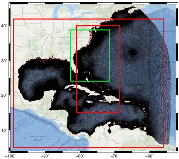
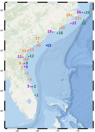
Figure 2.1 NHC best track for Matthew (black line and diamonds), along with observation locations (circles) on the U.S. southeast coast. High-water marks are not shown. The storm center positions are shown every 6 hr and color-coded to categories on the Saffir-Simpson scale. The storm positions are labeled in dates/times relative to UTC. The observation locations are color-coded to indicate whether they have data for meteorology (MET), waves (WH), and/or water levels (WL). . . 12 Figure 2.2 Coverage area of the WF (green) and OWI (red) wind grids over

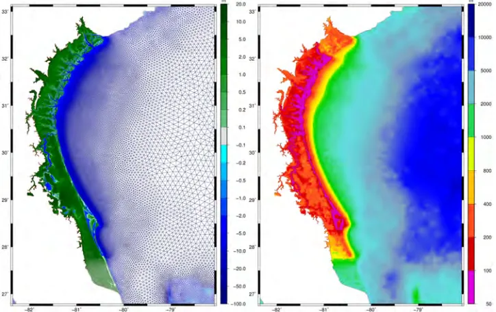
the HSOFS unstructured mesh (black). . . 16 Figure 2.3 The HSOFS mesh topography and bathymetry (m relative to

LMSL), contoured on the mesh elements (left figure). Colored boxes indicate specific regions as shown on the right: The Pam-lico Sound, North Carolina (pink), the Cooper and Savannah Rivers along the South Carolina-Georgia coast (orange) and Upper Florida showing the Fernandina Beach and St. Johns River (red). . . 19 Figure 2.4 Variation of offset values (m) along the U.S. southeast coast.

Ad-justments are shown for local sea level rise (dashed), steric effects (dotted), and total offset (solid). . . 21 Figure 2.5 Locations of selected stations for comparison of surface pressures,

wind speeds, significant wave heights and water levels. The points are color coded as in Figure 2.1 and numbered from south to north. 23 Figure 2.6 Hindcasts of wind speeds (m/s) during Matthew along the U.S.

southeast coast. Rows correspond to: (top) 0800 UTC 07 October, approximately 31 hours before landfall; (second from top) 2000 UTC 07 October, approximately 19 hours before landfall; (second from bottom) 1500 UTC 08 October, approximately at landfall; and (bottom) 0600 UTC 09 October, approximately 15 hours after landfall. Columns correspond to: (left) GAHM; (center) WF; and (right) OWI. Black lines represent the storm track for each source. 24 Figure 2.7 Time series of pressure deficits in hPa (left column) and wind speeds

(14)

Figure 2.8 Contours of water levels (m relative to NAVD88) and vectors of OWI wind speeds (m/s) during Matthew along the U.S. southeast coast. Times correspond to: (top left) 0800 UTC 07 October, approximately 31 hours before landfall; (top right) 1700 UTC 07 October, approximately 22 hours before landfall; (center left) 0200 UTC 08 October, approximately 13 hours before landfall; (center right) 0800 UTC 08 October, approximately 7 hours before landfall; (bottom left) 1500 UTC 08 October, approximately during landfall; and (bottom right) 0600 UTC 09 October, approximately 15 hours after landfall. . . 30 Figure 2.9 Time series of water levels (m relative to NAVD88) at 12 locations

shown in Figure 2.5. Observed values are shown with gray circles, and predicted values using OWI (solid). . . 31 Figure 2.10 Locations (top row) and scatter plots (bottom row) of HWMs and

peak hydrograph values during Matthew. Columns correspond to: (left) GAHM; (center) WF; and (right) OWI. Colors indicate error expressed as a percentage of observed value. Green points indicate errors within 10%; yellow and light blue indicate errors between 10% and 25%; orange and dark blue indicate errors between 25% and 50%; and red and purple indicate errors over 50%. The thick gray and black lines representy=xand best-fit lines, respectively. Statistical metrics are shown in Table 2.2. . . 33 Figure 2.11 Nonlinear interactions on the U.S. southeast coast during Matthew.

Columns correspond to: (left) positive maximum values and (right) negative maximum values. OWI was used as the source of mete-orological forcing for the simulations with only winds, and winds and tides together. Boxes indicate the location of the region shown in Figure 2.12. . . 36 Figure 2.12 Nonlinear interaction terms during Matthew at three locations

along the Blackbeard Creek, south of Savannah, Georgia. Columns correspond to: (left) location of stations and (right) time-series of water levels (m relative to NAVD88) with line types correspond-ing to: (solid) total water levels, (dashed-dotted) surge only, (dot-ted) tides-only, and (dashed) nonlinear terms. OWI was used as the source of meteorological forcing for the simulations with only winds, and winds and tides together. . . 37 Figure 2.13 Change in maximum water levels on delaying the storm by: (a)

(15)

Figure 2.14 Variation in maximum water levels along the coastline on altering the storm timing (top) and forward speed (bottom). Water levels during the standard Matthew run are indicated by black solid lines and those from perturbations are shown using grey color with line types (solid, dashed, dotted or dashed-dotted) as indicated in the figure legends. OWI was used as the source of wind forcing for all these simulations. . . 40 Figure 2.15 Change in maximum water levels on changing the forward speed

of the storm: (left) decreasing by 50%, (center) increasing by 50%, and (right) increasing by 100%. OWI was used as the source of wind forcing for all these simulations. The coastline is shown in black and the mesh boundary in brown. . . 41

Figure 3.1 Resolution (m) in the North Carolina in the HSOFS (top) and NC9 (bottom) meshes. . . 48 Figure 3.2 Differences in bathymetry and topography (m) between the higher

resolution (left) and the coarser resolution (right) meshes used in the idealized channel test case. Blue contours indicate bathymetry and the zero contour represents the coastline. . . 49 Figure 3.3 Water levels (m) in the two meshes. Columns correspond to: (left)

finer and (right) coarser meshes. Rows correspond to water levels at the (top) peak flood stage and (bottom) peak ebb stage of the tides. . . 50 Figure 3.4 Bathy-topo (left) and resolution (right) in metres, along the

Sa-vannah River in the HSOFS mesh. The points indicate locations where time series of water levels are shown in Figure 3.5. . . 52 Figure 3.5 Time series of water levels (m relative to NAVD88) at 6 locations

shown in Figure 3.4. Observed values are shown with gray circles, and predicted values using black lines. . . 52 Figure 3.6 Difference in maximum water levels (m) between the HSOFS and

NC9 meshes corresponding to the 58th advisory. The hurricane track is shown in black. . . 53 Figure 3.7 Maximum water levels (m) predicted using the HSOFS (left) and

NC9 (right) meshes, corresponding to the 58th advisory. The hur-ricane track is shown in black. . . 54 Figure 3.8 Bathymetry and topography (m) in the NC9 mesh. . . 56 Figure 3.9 Bathymetry and topography in m (top), and resolution in m

(bot-tom) in the SC mesh. . . 57 Figure 3.10 Bathymetry and topography in m (left), and resolution in m (right)

in the GANEFL mesh. . . 58 Figure 3.11 Bathymetry and topography in m (left), and resolution in m (right)

(16)

Figure 3.12 Bathymetry and topography in m (left), and resolution in m (right) in the SFL mesh. . . 60 Figure 3.13 Maximum of the maximum water levels (m) from each storm

sim-ulation. The hurricane tracks are shown in black and the mesh-boundary in brown. . . 62 Figure 3.14 Difference in the GANEFL mesh-boundary after removing vertices

with elevations over 5 m. The boundaries before and after the cut down is shown in brown and green, respectively. . . 63 Figure 3.15 Merging the SFL and open-water meshes: (1) the open water mesh

without the buffer and SFL regional mesh, (2) the SFL regional mesh cut at the 30 m bathymetric contour, and (3) the buffer mesh used to provide a smooth transition in element spacing between 1 and 2. The elements and boundaries are shown using black trian-gles and lines respectively. . . 64 Figure 3.16 FEMA-SAB mesh bathymetry and topography (m relative to

NAVD88) contoured on the mesh elements. Colored boxes indi-cate specific regions as shown in Figure 3.18. . . 67 Figure 3.17 Element spacing (m) along the U.S. southeast coast in the (left)

FEMA-SAB mesh and (right) HSOFS mesh. . . 68 Figure 3.18 Bathymetry and topography (m) contoured on the mesh elements

at locations represented by coloured grids in Figure 3.16. Columns correspond to: (left) FEMA-SAB mesh, and (right) HSOFS mesh. Rows correspond to: (top) Saint Lucie Inlet, FL, (center) Up-stream Savannah River along the GA-SC border, and (bottom) Outer Banks, NC. The FEMA-SAB mesh bathymetry is relative to NAV888, whereas the HSOFS mesh values are referenced to LMSL). 69 Figure 3.19 Variation of horizontal eddy viscosity ( m2 _s−1_{) along the U.S.}

southeast coast in the FEMA-SAB mesh. . . 73 Figure 3.20 Variation of Tau0 (s−1) along the U.S. southeast coast in the

FEMA-SAB mesh. . . 74 Figure 3.21 Variation of ManningsN (m s−1/3) along the U.S. southeast coast

in the FEMA-SAB mesh. . . 75 Figure 3.22 Variation of surface directional effective roughness length (m) along

the U.S. southeast coast in the FEMA-SAB mesh, corresponding to the 60 degree direction. . . 76 Figure 3.23 Variation of VCanopy (unitless) along the U.S. southeast coast in

the FEMA-SAB mesh. . . 77 Figure 3.24 Variation of elemental slope limiter (unitless) along the U.S.

(17)

Figure 3.25 NHC best track for Florence (black line and diamonds), along with observation locations of water levels (blue circles) on the U.S. southeast coast. High-water marks are not shown. The storm cen-ter positions are shown every 6 hr and color-coded to categories on the Saffir-Simpson scale. The storm positions are labeled in dates/times relative to UTC. . . 80 Figure 3.26 Time series of water levels (m relative to NAVD88) at the 12

locations shown in Chapter 2. Observed values are shown with gray circles, and predicted results using black lines with line types corresponding to: (solid) FEMA-SAB mesh, and (dashed-dotted) HSOFS mesh. . . 83 Figure 3.27 Locations of selected stations for comparison of water levels. The

points are numbered from south to north. . . 84 Figure 3.28 Time series of water levels (m relative to NAVD88) at the 10

lo-cations shown in Figure 3.27. Observed values are shown with gray circles, and predicted results using black lines with line types corresponding to: (solid) FEMA-SAB mesh, and (dashed-dotted) HSOFS mesh. . . 85 Figure 3.29 Locations (top row) and scatter plots (bottom row) of HWMs and

peak hydrograph values during Matthew. Colors indicate error expressed as a percentage of observed value. Green points indicate errors within 10%; yellow and light blue indicate errors between 10% and 25%; orange and dark blue indicate errors between 25% and 50%; and red and purple indicate errors over 50%. The thick gray and black lines representy=xand best-fit lines, respectively. Statistical metrics are shown in Table 3.2. . . 88 Figure 3.30 Locations of selected stations for comparison of water levels. The

points are numbered from north to south. . . 90 Figure 3.31 Time series of water levels (m relative to NAVD88) at the 10

(18)

Figure 3.32 Locations (left column) and scatter plots (right column) of HWMs and peak hydrograph values during Matthew. Rows correspond to: (ltop) FEMA-SAB mesh; and (bottom) HSOFS mesh. Colors indicate error expressed as a percentage of observed value. Green points indicate errors within 10%; yellow and light blue indicate errors between 10% and 25%; orange and dark blue indicate errors between 25% and 50%; and red and purple indicate errors over 50%. In the location plots, the mesh-boundary is shown in brown. For the scatter plots, the thick gray and black lines representy =xand best-fit lines, respectively. Statistical metrics are shown in Table 3.2. 94

Figure 4.1 Panels showing (top row) bathymetry (m) and (bottom row) wa-ter levels (m) from the Mixed simulation on the example case. Columns correspond to: (left) the digital elevation model; (cen-ter) coarse mesh; and (right) fine mesh. The water levels shown are for: (bottom-center) at the end of the coarse part ofMixed be-fore the switch, and (bottom-right) at the beginning of the fine part ofMixed after the switch. (The water levels in (bottom-center) are interpolated/extrapolated to become the water levels in (bottom-right).) Black dots indicate locations of the points where water levels are shown in Figure 4.2, and triangles indicate locations of mesh elements. . . 103 Figure 4.2 Boundary forcing (m) and water levels (m) for the simple example.

On the top-left is the variation in input forcing with line types cor-responding to (dotted) tides-only, (dashed) surge-only, and (solid) tides plus surge. The other three plots indicates time-series of wa-ter levels (m) at the three locations shown in Figure 4.1 with line types corresponding to: (solid)Coarse, (dotted)Fine, and (dashed-dotted)Mixed. . . 104 Figure 4.3 Scatter plots of HWMs and peak hydrograph values during

(19)

Figure 4.4 Contours of wind speeds (knots) during Florence along the NC coast. The time corresponds to 0000 UTC 13 September 2018 (36 hours before landfall), when switching between the coarse and fine meshes was done in the Mixed approach. Red dot indicates the point used to calculate distances to the maximum wind isotachs in Table 4.3 . . . 111 Figure 4.5 Difference in maximum water levels (m) between: (a)Coarse and

Fine, (b)Coarse andMixed, (c)Mixed andFine, and (d)Coarse and Mixed, but only locations where theCoarse was dry andMixed was wet. The coastline is shown in black and the fine-mesh boundary in brown. . . 114 Figure 4.6 Columns correspond to: (left) Bathymetry and topography in the

coarse (upper) and fine (bottom) meshes; and (right) Time Series of water levels (m) at the 3 locations indicated by red dots, with line types corresponding to: (solid) Coarse, (dotted) Fine, and (dashed-dotted) Mixed. . . 116 Figure 4.7 Columns correspond to: (left) Difference in maximum water levels

(m) between Coarse; and Mixed and (right) Only locations where the Coarse was dry and Mixed was wet. The coastline is shown in black and the fine-mesh boundary in brown. Black dots indicates the locations of the three points in Figure 4.6 . . . 117

Figure 5.1 Time series of water levels (m relative to NAVD88) at 6 locations along the US coastline (south to north) during Matthew. Rows correspond to: (top) stations on East-Florida coastline; (center) stations along the GA-SC coastline; and (bottom) stations along the NC coastline. Columns correspond to: (left) station where the impact of the storm was first recorded; and (right) station where the impact was last recorded on that particular coastline. Observed values are shown with gray circles. Blue and red lines indicate the starting and ending time of storm’s impact on water levels along that particular coastline respectively. . . 121 Figure 5.2 Locations of eye of the Matthew (diamonds) along with

(20)

Figure 5.3 Application of the approach during Matthew. Black triangles(a) indicate the elements of the HSOFS mesh. Solid black lines (b to f) indicate the part of the single high resolution mesh (black dashed lines) to be used at that particular point in time. Times T1 to T5 are the same as in Figures 5.1 and 5.2. The NHC best track for Matthew is shown by red lines and the storm-eye by diamonds. . . 125 Figure 5.4 Watershed boundaries for the U.S. southeast coast. Orange dots

indicate points that will be used to trigger switching between the meshes. . . 128 Figure 5.5 High-resolution coverage of the WSB307+306+305 mesh. The

mesh-elements are shown as black triangles, the mesh-boundary in green, and the orange dots indicates watershed boundary points as in Figure 5.4. . . 129 Figure 5.6 Time series of water levels (m relative to NAVD88) at the 10

loca-tions shown in Figure 5.4. . . 130 Figure 5.7 Time series of wind speeds (m/s) at the 10 locations shown in

Figure 5.4. . . 131 Figure 5.8 Time series of significant wave heights (m) at the 10 locations shown

in Figure 5.4. . . 132 Figure 5.9 Panels of: (left) Maximum water levels (m, NAVD88) for the

HSOFS Fine simulation; and (right) difference in maximum wa-ter levels (m) between the HSOFSTest and Fine simulations. The

coastline is shown in black and the mesh-boundary in brown. . . . 135 Figure 5.10 Maximum water levels (m, NAVD88) from the Fine simulation

(top-left), and differences in maximum water levels (m) as com-pared to theFineresults for: (top-right)FEMA-SABACC;

(bottom-left) FEMA-SABOPT; and (bottom-right) FEMA-SABEFF

(21)

Chapter 1 Introduction

Coastal regions are under a constant threat of property damage and casualties from

hurricanes, tsunamis, Nor’easters, and winter storms. Sustained winds and heavy rainfall

are not the only deadly factors during these natural hazards. The greatest threat to life

comes in the form of storm surge, measured as the height of the water above the normal

predicted astronomical tide. In flat regions, this may lead to intrusion of the salt water 10 to 20 miles inland (Conner et al., 1957). This flooding can also be accompanied by

erosion processes due to wave action, including breaching of barrier islands. Large-scale

features that would influence this surge include: the intensity, size, speed, and path of

the storm; the general configuration of the coastline; bottom topography near the coast;

and the stage of the astronomical tide (Harris, 1956; Reid et al., 1954). There can be

also small-scale features that affect the surge locally, such as convergence or divergence

in bays and estuaries, local wind-setup, seiching, etc.

The coastal populations on every continent exploded as global trade flowed through

international ports, creating jobs and economic growth. In 2001, more than 50 percent of

the world population lived within 200 km of the coastline (Tibbetts, 2002; Creel, 2003). Presently, 44 percent of the world’s population lives within 150 km of the coast (UN Atlas

of the Oceans, 2018). In the U.S., more than 39 percent (123.3 million people) of the

population lived in coastal shoreline counties in 2010 (NOAA et al., 2013). These

loca-tions also had the highest population density of 446 persons per square miles, compared

to the average U.S. density of 105 persons per square miles. With this ever-increasing

growth and development of coastal areas, greater damage to property and loss of life

(22)

The development and implementation of numerical models allows in the prediction of

these natural hazards so their potential effects can be understood and lives and property

can be protected from future storms.

Storm surge forecasting begin as early as the 1950s when the central pressure of

cyclones was used to estimate the maximum surge height (Hoover, 1957; Conner et

al., 1957). Improvements to these methods included using wave heights and stratifying

the cyclones according to their wind direction (Tancreto, 1958), employing multistation

surge models (Pore, 1964) and using approach paths (Chan et al., 1979). Recognizing

the complexity of surge forecasting, Harris (1963) developed a computer-aided empirical

model that included pressure effect, direct wind effect, Coriolis force, waves and rainfall as processes affecting storm surge. His first approximation showed that the effects of the

Coriolis force, waves, and wind set-up at sea are all proportional to the wind stress, and

that the wind stress is proportional to the pressure gradient. Also in general, rainfall was

observed to be correlated with below-normal pressures, resulting in all five factors being

directly related to pressure gradients.

Advances in computing power allowed the inclusion of more parameters and usage of

more complex equations, leading to development of the Special Program to List

Ampli-tude of Surge from Hurricanes (SPLASH) (Jelesnianski, 1972). This approach computed

peak surge via nomograms that used maximum wind, radius of the maximum wind, direction of landing, bathymetry, and central pressure data. The Federal Emergency

Management Agency (FEMA) SURGE Model (Dresser et al., 1985) was first introduced

in 1976 as the TTSURGE Model, and uses an explicit, two-dimensional, space-averaged,

finite-difference scheme to simulate the surges caused by hurricanes. Inputs to the model

include the bathymetry, coastline configuration, boundary conditions, bottom friction,

and other flow resistance coefficients. Also required are the surface wind stress and

at-mospheric pressure distributions of a hurricane. The model uses a rectangular grid to

represent the area of interest and usually employs a nested grid system so that greater

detail can be added along the coastline. Hurricane Audrey of 1957 was successfully sim-ulated using the model and the results showed good agreement with the flood records

(Suhayda et al., 1988).

The Sea, Land, Overland Surge from Hurricane (SLOSH) model (Jelesnianski et al.,

1992) was later designed by the National Weather Service to estimate storm surge heights

(23)

atmospheric pressure, size, forward speed, and track data. During a hurricane, the

po-tential surge for an area is calculated by running the model with hypothetical hurricanes

with various landfall directions and locations, Saffir-Simpson categories, forward speeds,

sizes, and tide levels. The envelope of high water from each such run is then combined to

create worst case scenario to aid in hurricane evacuation plans. Although useful in

fore-casting and computationally fast, the spatial coverage of each SLOSH grid only ranges

from an area the size of a few counties to a few states. But larger domains are needed for

capturing large-scale processes and improved accuracy (Blain et al., 1994; Westerink et

al., 1994). Also the use of a structured mesh can limit the ability for localized resolution

and therefore potentially hampers accuracy in SLOSH (Kerr et al., 2013).

Coastal morphological features like inlets, lagoons, barrier islands and shoreline

con-figuration have a great influence on inundation. The accuracy of flooding predictions thus

depends on whether the model has sufficient resolution to resolve these features. Because

it is difficult for finite difference models with structured grids to represent such fine

fea-tures, finite element models using unstructured grids are employed in accurate storm

surge forecasting. ADvanced CIRCulation (ADCIRC) (Luettich et al., 1992; Luettich

et al., 2004; Westerink et al., 2008) is a depth-integrated, shallow-water, finite-element

model capable of simulating tidal circulation and storm-surge propagation over large

com-putational domains. ADCIRC is used by FEMA in the development of flood insurance rate maps and by the U.S. Army Corps of Engineers (USACE) for navigation and storm

protection projects. The National Oceanic and Atmospheric Administration (NOAA)

also uses ADCIRC for tidal calibrations and incorporation into its vertical datum

trans-formation software VDatum. The use of unstructured meshes in ADCIRC allows the

usage of triangular finite elements of varying sizes to represent complex coastal features,

barrier islands and internal barriers. This also permits for gradation of the mesh that

increases feature detail when moving from the deeper ocean, onto the continental shelf,

into estuaries and marshes, and over low-lying coastal floodplains. More details of the

model are given in Chapter 2.

These unstructured meshes can be still be large, composing of millions of elements.

For example, the SL18TX33 mesh (Hope et al., 2013) uses 9 M vertices and 18 M

ele-ments to provide a detailed description of coastal floodplains of Alabama, Mississippi,

Louisiana, and Texas. Element sizes varies from 20 km or larger in the Atlantic Ocean

(24)

features. Thus, although these models provide reliable and accurate results by virtue of

their high-resolution description of coastal features, simulations can be computationally

expensive, requiring several hours even on thousands of computational cores (Dietrich

et al., 2012). This is a challenge in storm surge modeling, especially in forecasting

appli-cations where model predictions are required on the order of 1 hr or so, to aid emergency

mangers in decision-making during a hurricane.

The present study describes a multi-resolution approach to cut down the total

compu-tational cost of running unstructured-mesh, storm surge models. The study begins with

an application of the state-of-the-art in storm surge modeling to predict coastal flooding

along the the U.S. southeast coast during Hurricane Matthew (2016). In the later chap-ters, I apply a multi-resolution method that permits the use of higher-resolution meshes

to increase the accuracy of flooding predictions. This method will also help in decreasing

the simulation time by using high-resolution only when required. This is attained by

us-ing multiple meshes with different levels of resolution at different times in the simulation.

Higher-resolution meshes will be used to resolve coastal inundation only when necessary

rather than during the entire simulation. An overview of each of the individual chapters

of this dissertation is provided below.

Storm surge and flooding due to hurricanes can cause significant damage to property,

loss of life, and long-term damage to coastal landscapes. Hurricane Matthew (2016) was a Category-5 storm that impacted the southeastern U.S. during October 2016, moving

mostly parallel to the coastline from Florida through North Carolina. In Chapter 2,

the tightly-coupled ADCIRC+SWAN storm surge forecasting model is used to simulate

Matthew’s effects on this long coastline, and then validated against extensive

observa-tions of surface pressures, wind speeds, waves, and water levels. Data-assimilated wind

products was found to better represent Matthew’s effects as compared to the

paramet-ric vortex model, which is based on best-track information from the National Hurparamet-ricane

Center. A relatively-coarse unstructured mesh having an average coastal resolution of

500 m, and having a coverage that included the coastal floodplains impacted by Matthew was then used to predict Matthew’s impact on the U.S. southeast coast. Even with this

relatively-coarse mesh, the modeled results showed good agreement to observations for

waves, water levels and high water marks, thus proving the capability of the coupled

ADCIRC+SWAN model to provide accurate coastal flooding predictions.

(25)

above-mentioned coarse-resolution mesh were comparable to that using meshes with much

higher-resolution, there were localized regions like rivers along the South Atlantic Bight,

sound-side of barrier islands in North Carolina, etc., where the errors where larger. This

was attributed to its larger coastal resolution, which is insufficient to represent smaller

features like channels, tidal inlets and dune crests. Therefore a mesh with detailed

cov-erage of floodplains on the U.S. southeast coast is developed and validated in Chapter 3.

This mesh will then be also used in later chapters for a coarse-grain mesh adaptivity, by

including the floodplains only when required.

This high-resolution mesh was created from existing regional meshes, which were

developed by FEMA for flood risk mapping. It has a resolution of less than 100 m in most places along the southeastern U.S. coastline with the element spacing going

down to less than 10 m in some of the smaller channels in South Florida. This mesh

was then tested by running ADCIRC+SWAN simulations of two storms that impacted

the U.S. southeast coast in different ways. For both these storms, the predictions of

water levels were either better or comparable to predictions using the coarse-resolution

mesh mentioned above, meanwhile flooding a larger number of observed-stations. The

main differences occurred inland away from the coastline, where it better captured the

tidal impacts and/or had a better match to the peak water levels, due to its detailed

representation of topography and bathymetry. Thus although this mesh has roughly three times the number of elements as that of the coarse-resolution mesh, its predictions

were a better match to observations, especially inland.

In Chapter 4, a method to reduce the computational workload of storm surge models

is proposed. Although different methods to increase resolution in storm surge models can

be seen in literature, the proposed approach is a first of its kind. Rather than using a

high-resolution mesh throughout the simulation, high-resolution can be turned on depending on

where the storm is located at a particular point in time. A coarse-resolution mesh without

extensive coastal detail is used when the storm is far away. As the storm approaches the

region of interest, results are mapped on to a high-resolution mesh. The simulation then continues on the fine mesh providing high-accurate results for that coastline. A save is

tine is also achieved as the use of a highly-refined mesh is avoided when the storm is far

away. The approach was tested in the case of two storms with different parameters like

track, intensity, etc, and results indicated a gain in accuracy and efficiency as compared

(26)

In Chapter 5, the multi-resolution approach described in Chapter 4 is again applied to

hindcasts of Hurricane Matthew along the U.S. southeast coast. But rather than using a

single switch between the coarse and the full resolution mesh, multiple smaller

fine-resolution meshes will be used depending on the storm’s impact area at different points

in time. Questions about how best to apply the approach given information about the

storm and predicted values of water levels, wind speeds, and wave heights will be explored

using three simulations, each targeting a different level of accuracy and efficiency. Results

from these simulations indicate how to achieve an optimum balance between accuracy

and efficiency using the approach, and the best ways to choose combinations of meshes for

representing the storm’s impact region. Thus, an efficient use of the proposed method during forecasting can allow for a more accurate and timelier guidance. Finally, the

(27)

Chapter 2 Influence of Storm Timing and

Forward Speed on Tides and Storm

Surge during Hurricane Matthew

2.1 Overview

In this chapter, the sensitivity of surge predictions to timing and forward speed of a

storm are analyzed in the context of Hurricane Matthew (2016). First, the effects of

Matthew on the southeastern U.S. coastline are explored by performing hindcasts of a

coupled hydrodynamic-wave model, using three sources of atmospheric forcing and an unstructured mesh with a widespread coverage that includes the areas impacted by the

storm. Then, the contribution of nonlinear interactions between surge and tides to the

spatial variability of Matthew’s effects on total water levels is analyzed. Finally, the

influence of storm timing and forward speed on tides and surge during Matthew are

separately analyzed. This chapter has been published in Ocean Modelling as Thomas et al. (2019).

2.2 Introduction

Matthew was a tropical cyclone that reached Category-5 hurricane status on the

Saffir-Simpson hurricane wind scale during 2016. Matthew affected about 1900 km of coastline

(28)

(Stewart, 2017). Between 1900 UTC 06 October when the storm was located offshore of

Miami, Florida, and 0600 UTC 09 October when it was located offshore of Cape Hatteras,

North Carolina, Matthew remained close to the coast and moved along a shore-parallel

track (Figure 2.1) with a relatively-slow forward speed of 5 to 7 m/s. Observations indicate large variations in peak water levels all along the U.S. Atlantic coast, and we

hypothesize that this was caused by the storm’s slower forward speed and shore-parallel

track, which allowed it to interact with different stages in the tidal cycle at different

locations and over several days.

Several studies have examined the interactions between tides and surge. In the 1950s,

Proudman developed theoretical solutions for the propagation of an externally forced tide and surge into an estuary of uniform section (Proudman, 1955; Proudman, 1957) and

also identified the tendency of peak surge to most often occur on high tides, which was

later confirmed (Rossiter, 1961; Prandle et al., 1978). Tides and surge can also interact

nonlinearly, thus causing the water levels to be even higher or lower than their individual

contributions would suggest, due to feedbacks through bottom friction, shallow-water

effects, and advection (Wolf, 1978). Nonlinear parameterization of bottom stress was

found to the primary contributor to nonlinear tide-surge interactions along the

Queens-land coast of Australia (Tang et al., 1996), on the east coast of Canada and northeastern

United States (Bernier et al., 2007), and along the Fujian coast (W. Zhang et al., 2010). Along the southeast coast of the United States, Coriolis acceleration was found to be a

significant contributing factor to these perturbations (Valle–Levinson et al., 2013; Feng

et al., 2016). The magnitude of these interactions can be large, reaching as high as

70% of the tidal amplitudes (Rego et al., 2010) along the Louisiana-Texas coast during

Hurricane Rita, and 74 cm (Idier et al., 2012) for storms in the English channel. The

tide-surge nonlinearities were also large with a mean absolute value of 60% of the tide

magnitude (Lin et al., 2012) for synthetic surge events in New York Harbor, and at least

15−20% for idealized cyclone tracks and straight coastlines representing the west coast

of India (Poulose et al., 2017).

It can be challenging to include these nonlinear interactions in surge predictions.

Flood risk studies typically represent the hurricane climate by using the Joint Probability

Method (JPM) with synthetic storms to determine the flooding at various return periods.

The effect of tides can be a crucial factor in these studies. For studies looking at smaller

(29)

addition to the JPM integral error term (Niedoroda et al., 2010). Other studies included

tides into the JPM analysis by randomly adding tidal heights to the surge response (Ho

et al., 1975; Blanton et al., 2012; U.S. Army Corps of Engineers, 2018). However, these

additions do not incorporate the often-large effect of the nonlinear interactions between

the surge and tides. The present study quantifies these interactions along the entire U.S.

southeast coast during Matthew, including their variation from the continental shelf into

the estuaries. The representation of coastal floodplains is larger than in previous studies

and can allow the flooding from the shore-parallel storm to interact with multiple phases

of the tides.

The effects of storm parameters like size, landfall location, wind speeds, and direction of approach on surge have also been studied previously ((Weisburg et al., 2006; Irish et

al., 2008; Sebastian et al., 2014)). The effect of storm forward speed can vary. The surge

can be greater for a faster storm, e.g., for a standard hurricane on a representative shelf

(Jelesnianski, 1972). Along the Louisiana-Texas shelf for Hurricane Rita, increasing the

forward speed of the storm caused higher surges but smaller total flooded volumes (Rego

et al., 2009). But the surge and inundation areas can also be greater for a slower storm,

e.g., for the estuaries of North Carolina (Peng et al., 2004), and for the Dutch coast (N. J.

Berg, 2013). For the Charleston Harbor in South Carolina, although a slower storm can

produce larger inundation areas, whether or not it can produce larger surge depends on the faster storm’s speed and the distance of the track from the harbor (Peng et al., 2006).

While these studies have identified the vulnerability of the coastline to hurricane storm

surge under different scenarios, they considered small regions or idealized coastlines, and

storms that moved perpendicular to the coastline. The present study uses Hurricane

Matthew’s track along the coast from Florida to North Carolina to examine how the

forward speed of a shore-parallel storm affects the surge and inundation along a complex

estuarine coastline and coastal floodplain.

This study uses the coupled ADCIRC+SWAN model, which has proven to be accurate

in flood predictions in many coastal systems (Hope et al., 2013; Suh et al., 2015; Dietrich et al., 2018). The model utilizes an unstructured, finite-element mesh developed for

surge and tide predictions for the U.S. Atlantic and Gulf coasts (Riverside Technology

et al., 2015). The unstructured mesh can represent a large domain, while using sufficient

resolution to represent the complex shoreline. This combination allows for comprehensive

(30)

influence of storm timing and forward speed on flooding for a shore-parallel storm in a

large domain. The goals are addressed by (a) validating model predictions of winds, and

water levels during Matthew on a mesh with floodplain coverage over a large extent, (b)

quantifying the contributions of nonlinear interactions to the total water levels, and (c)

quantifying the differences in flooding due to differences in the storm’s forward speed

and time relative to the tidal cycle.

2.3 Hurricane Matthew

2.3.1 Synoptic History

Matthew began as a tropical wave off the west coast of Africa on 23 September 2016

(Stewart, 2017), and by 1200 UTC 28 September, measurements indicated a tropical

storm formation about 27 km west-northwest of Barbados. Moving into the Caribbean

Sea, Matthew attained hurricane status on 1800 UTC 29 September about 300 km

north-east of Cura¸cao. Matthew then turned west-southwest and intensified to an estimated

peak intensity of 75 m/s (Category-5) on 0000 UTC 1 October. Over the next few days, the storm weakened to a category 4 status as it moved northward and made landfall with

peak wind speeds of 66 m/s over Haiti (1100 UTC 4 October) and 59 m/s over Cuba (0000 UTC 5 October). By 1200 UTC 6 October, the storm brought hurricane-force

winds and flooding rains to most of the central and northwestern Bahamas with a peak

wind speed of 64 m/s. The category 4 hurricane made landfall near West End, Grand Bahama Island, around 0000 UTC 7 October (Stewart, 2017).

A broad eastward-moving mid-latitude trough located over the central United States

then caused Matthew to turn toward the north-northwest (Stewart, 2017) and impact

much of the southeastern U.S. (Figure 2.1). The storm weakened to a category 3 hurricane around 0600 UTC 7 October about 64 km east of Vero Beach, Florida, and to a category

2 hurricane by 0000 UTC 8 October about 92 km east-northeast of Jacksonville Beach,

Florida. As the storm moved northward, its wind field expanded causing

hurricane-force wind gusts across the coastal regions of southeastern Georgia and southern South

Carolina. The mid-latitude trough then caused the storm to weaken to a category 1

status (Stewart, 2017). Moving nearly parallel to the coast of South Carolina, Matthew

(31)

The center of the hurricane then traveled offshore of the coast of South Carolina and

remained just offshore of the coast of North Carolina through 9 October. Contributions

from Matthew’s tropical moisture, the ongoing extratropical transition and an increasing

pressure gradient from an approaching cold front caused sustained hurricane-force winds

over the Outer Banks and significant sound-side storm-surge flooding during the early

hours of 9 October. Matthew lost its tropical characteristics by 1200 UTC 9 October, as

it moved away from the U.S (Stewart, 2017).

2.3.2 Extensive Observations along U.S. East Coast

Matthew’s effects on surface pressures and wind speeds, offshore and nearshore waves,

and coastal water levels are well-described by observational data. Along the southeastern

U.S. coast from Florida through North Carolina (Figure 2.1), the National Oceanic and Atmospheric Administration (NOAA), the U.S. Geological Survey (USGS), and other

agencies collected information at hundreds of buoys, permanent and rapidly deployed

gauges and stations, and real-time sensors. Along the storm’s path, surface pressures

were observed at 283 locations, wind speeds and directions were observed at 66 locations,

and significant wave heights were observed at 16 locations (Table 2.1). Time series

observations at buoys and stations operated by the NOAA National Data Buoy Center

(NDBC) and the NOAA National Ocean Service (NOS) show how the peak,

10-minute-averaged wind speeds evolved during the course of the storm. Wave parameters were also

observed at many of these same locations.

These winds and waves caused setup and storm surge along the southeastern U.S.

coastline. NOS and USGS permanent and rapidly-deployed gauges collected observations;

time series of water levels at 501 locations and 612 high-water marks (HWMs) were

identified within the model extent. For the analyses herein, observations were omitted

that did not operate during the storm peak or that showed elevated water levels after

the storm due to freshwater run-off or wave run-up, thus leaving 289 time series and 464

HWMs to describe storm surge (Table 2.1). These observations are used to validate our

(32)

(33)

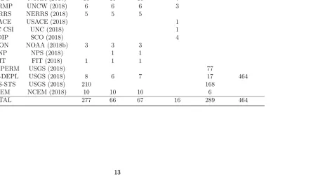
Table 2.1 Numbers of available observations for atmospheric, wave, and water-level responses to Matthew.

Surface Wind Wind Significant Water High Data Source Reference Pressure Speed Direction Wave Height Levels Water Marks

NOS NOAA (2018a) 19 19 19 21

NDBC NOAA (2017) 15 15 15 7

CORMP UNCW (2018) 6 6 6 3

NERRS NERRS (2018) 5 5 5

USACE USACE (2018) 1

UNC CSI UNC (2018) 1

CDIP SCO (2018) 4

ICON NOAA (2018b) 3 3 3

ENP NPS (2018) 1 1

FIT FIT (2018) 1 1 1

USGS-PERM USGS (2018) 77

USGS-DEPL USGS (2018) 8 6 7 17 464

USGS-STS USGS (2018) 210 168

NCEM NCEM (2018) 10 10 10 6

(34)

2.4 Methods

Predictions of waves and storm surge are sensitive to the atmospheric conditions used as

forcing to the model simulations. In this study, we evaluate forcings from three sources: a

vortex model based on storm parameters like the track, forward speed, and isotach radii; and two data-assimilated products available after the storm. Then the most-accurate

atmospheric forcing is used for a detailed hindcast of Matthew’s effects on water levels

throughout the southeastern U.S., via comparison with extensive observations. This

study uses the depth-averaged, barotropic version of ADCIRC, because the strong surface

stresses during storms causes the water column to be well-mixed in shallow nearshore

and coastal regions. This hindcast is then used as the basis for studies of the nonlinear

interactions between tides and surge, and of the effects of storm timing and forward

speed. In this section, details are provided about the three sources for surface pressure

and wind fields that were evaluated for hindcasts of Matthew, as well as the input settings for the coupled ADCIRC+SWAN model.

2.4.1 Surface Pressure and Wind Fields

Hydrodynamic predictions are analyzed with three sources of atmospheric forcing: a

pa-rameterized vortex model based on storm parameters from the National Hurricane Center

(NHC), and two data-assimilated products. For all three sources, the surface pressures

and wind velocities are developed (either by the parametric model or by interpolation

from the data-assimilated products) at the computational points in the model domain.

ADCIRC accounts for canopy cover and applies a surface roughness reduction factor

increases to full marine winds as overland regions are inundated (Kerr et al., 2013).

2.4.1.1 Parametric Vortex Model

It is common to use parametric vortex models to represent storm wind fields based on

limited input information (Xie et al., 2006; Hu et al., 2012; Hu et al., 2015). These

mod-els assume a hyperbolic radial pressure field that depends on the ambient and cyclone

central surface pressures, the radius to maximum winds, and the hurricane-shape

pa-rameter (Schloemer, 1954; Holland, 1980). Several parametric vortex models have been

(35)

(Mattocks et al., 2006; Mattocks et al., 2008; Dietrich et al., 2013a). The most complete

is the Generalized Asymmetric Holland Model (GAHM),which has been shown to be a

better representation than earlier versions (Gao et al., 2017), and to compare well with

observation-based analysis products and full-physics numerical models (Dietrich et al.,

2018; Cyriac et al., 2018). In this study, GAHM is used with the NHC Best Track storm

parameters for Matthew (Stewart, 2017) to generate surface pressures and wind speeds at

every computational point in the ADCIRC domain. Unlike the two atmospheric forcings

described below, GAHM is not data-assimilated and only represents the vortex, with no

far-field meteorological representation.

2.4.1.2 Data-Assimilated Atmospheric Products

Surface pressure and wind velocities from WeatherFlow Inc. (WF) were developed using

the Weather Research and Forecasting (WRF) model (Skamarock et al., 2008), which

can simulate weather processes at synoptic scales down to large eddy simulations at

microscales. During Matthew, 52 stations measured sustained wind speeds greater than

22 m/s, with 32 stations measuring gusts of at least 33 m/s. These observations were assimilated into fields of surface pressures and wind velocities.These fields cover a period from 2000 UTC 06 October 2016 until 2000 UTC 09 October 2016, at 10-min intervals.

The fields cover from latitude 24.15◦N to 38.67◦N and from longitude 83.55◦W to 72.02◦W with square elements of 96.12 arc-seconds (approximately 3 km north-south by 3 km

east-west). The surface pressures and wind velocities are interpolated in space and time to

the ADCIRC computational points within the WF domain (Figure 2.2).

The second source for data-assimilated products was Oceanweather Inc. (OWI), whose

fields are based on observations from anemometers, airborne and land-based Doppler

radar, airborne stepped-frequency microwave radiometer, buoys, ships, aircraft, coastal

stations and satellite measurements (Bunya et al., 2010). For Matthew, the Tropical PBL (TropPBL) model (Cardone et al., 1994; Thompson et al., 1996) was applied in

the core during the entire storm, with hand analysis overlay from 2100 UTC 06

Octo-ber 2016 until 1500 UTC 09 OctoOcto-ber 2016, to better represent the interaction of the

storm with the coast. The resultant wind and pressure fields are then subject to manual

kinematic analysis using the IOKA system to add features that are not well-resolved by

the TropPBL model, as well as in-situ, satellite, and aircraft data, into the final fields.

(36)

Figure 2.2 Coverage area of the WF (green) and OWI (red) wind grids over the HSOFS unstructured mesh (black).

above the ground/sea level with consideration to marine exposure. Lagrangian-based

interpolation is then used to produce fields at 15 min intervals. For use as atmospheric

forcing to hydrodynamic models, the surface pressure and wind fields are represented

with a lower-resolution basin grid and a higher-resolution region grid (Figure 2.2). The basin grid covers from latitude 5◦N to 42◦N and from longitude 99◦W to 55◦W with a spatial resolution of 0.25◦, whereas the higher-resolution region field covers from latitude 15◦N to 40◦N and from longitude 82◦W to 68◦W with a spatial resolution of 0.05◦, both covering a period from 0000 UTC 01 October 2016 until 0000 UTC 11 October 2016, at

(37)

2.4.2 Coupled Models for Nearshore Waves and Circulation

The storm-induced waves and circulation during Matthew must be predicted by models

that can represent their interactions over a wide range of temporal and spatial scales,

including coastal flooding into overland regions. We use the coupled SWAN+ADCIRC

models (Dietrich et al., 2011b; Dietrich et al., 2012), which have been validated

exten-sively for flooding during tropical cyclones (Bhaskaran et al., 2013; Hope et al., 2013;

Suh et al., 2015; Dietrich et al., 2018).z

The unstructured-mesh version of SWAN uses a sweeping Gauss-Seidel method to

propagate efficiently the wave action density (Booij et al., 1999; Zijlema, 2010). The

action balance equation is used to incorporate source/sink terms for nearshore wave physics, such as triad nonlinear interactions, bottom friction and depth-limited breaking,

in addition to deep-water physics of quadruplet nonlinear interactions and whitecapping.

The simulations in this study use SWAN version 41.01 with a time step of 600 s. The

spectral space is discretized using 36 directional bins with directional resolution of 10◦ and 40 frequency bins with a logarithmic resolution over the range 0.031 to 1.42 Hz. This logarithmic discretization of frequencies is based on the ratio of ∆f /f = 0.1 for the discrete interaction approximation of the quadruplet interactions (Hasselmann et al.,

1985). This spectral discretization and other physical and numerical settings are the

same as used in previous hindcast studies by the authors (Dietrich et al., 2011a; Dietrich et al., 2013b). To prevent excessive directional turning or frequency shifting at a single

vertex due to steep gradients in bathymetry or ambient currents, the spectral velocities

in SWAN are limited using a CFL restriction (Dietrich et al., 2013b) with an upper limit

of 0.25.

ADCIRC uses the continuous-Galerkin finite element method to solve the shallow

water equations on unstructured meshes (Luettich et al., 1992; Kolar et al., 1994;

Luet-tich et al., 2004; Dawson et al., 2006; Westerink et al., 2008). Water levels are

calcu-lated using the Generalized Wave Continuity Equation (GWCE), which is a combined

and differentiated form of the continuity and momentum equations (Kinnmark, 1986), whereas depth-averaged current velocities are determined from the vertically-integrated

momentum equations. For the simulations in this study, ADCIRC version 52.30.13 is

used in explicit mode with the lumped mass matrix form of the GWCE (Tanaka et al.,

2011). The bottom drag is applied using a depth-dependent quadratic friction law, with

(38)

al., 1992; Luettich et al., 2004). These Manning’s n values are also used by SWAN to compute roughness lengths based on the updated ADCIRC water levels at each mesh

vertex (Bretschneider et al., 1986; Madsen et al., 1988; Dietrich et al., 2011a). The

min-imum bathymetric height and friction-surface velocity required for wetting are 0.10 m and 0.01 m/s, respectively. The spatially-constant horizontal eddy viscosity for the mo-mentum equations was set to 50 m2 _s−1_{, and an ADCIRC time step of 1 s was used. The} wind drag coefficients on the water surface are calculated using the Garratt formulation

(Garratt, 1977; Westerink et al., 2008) with an upper limit of CD = 0.002, similar to previous studies (Dietrich et al., 2011a; Dietrich et al., 2012). The advective transport

terms were enabled to account for nonlinear interactions between surge and tides. The unstructured-mesh spectral wave model SWAN and the shallow water circulation

model ADCIRC were integrated into a coupled SWAN+ADCIRC model so they share

the same computational cores and the same unstructured mesh (Dietrich et al., 2011b;

Dietrich et al., 2012). ADCIRC interpolates the wind velocities and computes water levels

and velocities, and then supplies them to SWAN, which uses them in its computations for

evolution of spectral action density. At the end of each SWAN time step, wave radiation

stresses and their gradients are computed by SWAN, and then passed on to ADCIRC,

which applies them as surface stresses in its momentum equations. The coupling interval

is taken to be the same as the SWAN time step of 10 min.

2.4.3 Unstructured Mesh to Describe the Southeast U.S. Coast

This study uses the Hurricane Surge On-Demand Forecasting System (HSOFS) mesh,

which provides coverage of nearshore regions and coastal floodplains along the entire U.S.

coast from Texas through Maine (Riverside Technology et al., 2015). The widespread

coverage of the HSOFS mesh is possible because its local mesh resolution is typically

coarser than meshes for specific coastal regions. The mesh has an average resolution

of 500 m along the coast with some areas decreasing to a resolution of 150 m. At most

locations, the mesh extends inland to a smoothed version of the 10-m topographic contour

(Figure 2.3). It has a total of 1,813,443 vertices and 3,564,104 elements. Two primary data sources were used to provide bathymetry/topography: the USGS 1/9 arc second National Elevation Dataset (NED) Digital Elevation Model (DEM) (U.S. Geological

Survey, 2018) supplied overland topography and the NOAA East Coast 2012 (EC2012)

(39)

has been validated for 10 major tropical and extra-tropical storms covering a spectrum

of landfalls across the U.S. coast including Isabel, Katrina, Ike, and Sandy (Riverside

Technology et al., 2015). The HSOFS mesh is ideal for this study because its widespread

coverage includes the nearshore regions and floodplains impacted by Matthew along the

southeast U.S. coast.