Plaß, Julia (2018): Statistical modelling of categorical data under ontic and epistemic imprecision: contributions to power set based analyses, cautious likelihood inference and (non-)testability of coarsening mechanisms. Dissertation, LMU Münche

(1)

Statistical modelling of categorical data

under ontic and epistemic imprecision:

Contributions to power set based analyses,

cautious likelihood inference and

(non-)testability of coarsening mechanisms

Julia Irina Plaß

(2)

(3)

Statistical modelling of categorical data

under ontic and epistemic imprecision:

Contributions to power set based analyses,

cautious likelihood inference and

(non-)testability of coarsening mechanisms

Julia Irina Plaß

Dissertation

an der Fakult¨at f¨ur Mathematik, Informatik und Statistik

der Ludwig–Maximilians–Universit¨at M¨unchen

vorgelegt von

Julia Irina Plaß

aus N¨urnberg

(4)

(5)

Acknowledgement

I would like to express my sincere gratitude to everyone who contributed to this dissertation! A special thanks goes to . . .

. . . Thomas Augustin for the pleasant collaboration, motivation, trust, support and all the

very helpful advice, or in short, for the excellent supervision. Thank you for always taking time and encouraging me, especially when the feared ISIPTA deadline nears!

. . . In´es Couso and Frauke Kreuter for their willingness to fill the role of the external

reviewers and Helmut K¨uchenhoff and Volker Schmid for their willingness to be part of the examination committee.

. . . my coauthors Thomas Augustin, Marco Cattaneo, Paul Fink, Christian Heumann,

Aziz Omar, Norbert Sch¨oning and Georg Schollmeyer for the great collaboration.

. . . Marco Cattaneo for the kind invitation to the School of Mathematics and Physical

Sciences at the University of Hull. Thank you, Marco, for very helpful discussions, significantly pushing forward our project about reliable regression analysis. Moreover, I appreciate the hospitality of Andrea Wiencierz and Marco Cattaneo planning plenty of activities to make my time in England perfect!

. . . Francesca Biagini, my mentor in the LMUMentoring program. Thank you also for

the financial support that gave me the opportunity to present our work at several con-ferences. Meeting researchers from similar topics definitely inspired further research.

. . . Eyke H¨ullermeier and Sabine Zinn for the kind invitation to present our work in the

Intelligent Systems group at the University of Paderborn and the Leibniz Institute for Educational Trajectories, respectively. Thank you also for the fruitful discussions.

. . . the Research Data Center at the Institute for Employment Research, Nuremberg,

for the access to the PASS data. Moreover, I thank all organizers of the “mouse movement” study, in particular Malte Schierholz, for including our question(s).

. . . all former and current members of my working group: Thank you Andrea, Aziz,

Christoph, Eva, Georg, Johanna, Marco, Patrick, Paul and Thomas for the great collaboration, stimulating discussions at the research seminar, your unique indecision in the choice of restaurants and an unforgettable time!

. . . all remaining former and current colleagues at the Department of Statistics for the

excellent general atmosphere. Thank you, Jona and Sarah for the great breaks in the Eisbach, thank you for the ice-cream, Margret!

. . . “knorke” office 248! Thank you for all the singing, drumming, chocolate and the

jumps in the air. I would like to have you in my office forever!

. . . Ari, Basti, Carola, Christoph, Georg, Eva, Oscar and Silke for proofreading parts

of this thesis, especially Malte and Matthias for reading through the sections about survey statistics.

. . . the best family and the best boyfriend who always support me, understand me and are

(6)

(7)

Zusammenfassung

Grobe Daten, d.h. Daten, die nicht in der ursprünglich gewünschten Genauigkeit beobachtet werden, entstehen aus den verschiedensten Gründen. Beispielsweise kann es sein, dass Befragte sich nicht zwischen Antwortmöglichkeiten (wie z.B. Parteien) entscheiden können oder, dass sie – insbesondere bei sensitiven Fragen – nicht bereit sind, genauere Informationen preiszugeben. Während die Variable im ersten Beispiel von Natur aus impräzise Werte aufweist, liegt in der zweiten Situation ein impräziser Beobachtungsprozess eines präzisen Wertes zugrunde. Somit weisen die Fälle auf zwei sich grundsätzlich unterscheidende Interpretationen von groben Daten hin, die in der Literatur mit ontischer und epistemischer Datenimpräzision bezeichnet werden. Diese kumulative Dissertation verfolgt das Ziel einer vertrauenswürdigen statistischen Model-lierung grober Daten, welche die gesamte verfügbare Information – und nur diese – ausnutzt. Dabei werden eine grobe, kategoriale Responsevariable und präzise, kategoriale Kovariablen be-trachtet. Die Arbeit motiviert das Thema, indem das Erheben von groben kategorialen Daten als mögliche Strategie aufgezeigt wird, verschiedene bei der Beantwortung von Surveyfragen auftretende Fehler zu minimieren. Nach einer Einordnung der Arbeit in die allgemeine Li-teratur werden die eingehenden Beiträge zusammengefasst, Querverbindungen herausgearbeitet und Ideen für die weitere Forschung skizziert. Abschließend wird nochmals Bezug zur Survey-forschung genommen, wobei sich zeigt, dass die Vorschläge dieser Arbeit auch von aktuellen Entwicklungen, wie der Erhebung von Paradaten, profitieren. In die Dissertation geht ein Beitrag (Beitrag 1) ein, der sich mit ontischer und vier Beiträge (Beitrag 2 bis 5), die sich mit epistemischer Datenimpräzision befassen.

Durch Zulassen von Mehrfachantworten und die Betrachtung derselben als eigene Entit¨aten wird

inBeitrag 1 ein neuer Weg f¨ur den Umgang mit Antworten von Unentschlossenen aufgezeigt.

Dieser Wechsel des Zustandsraumes zur Potenzmenge des urspr¨unglichen Zustandsraumes wird

f¨ur das multinomiale Logitmodell und Klassifikationsb¨aume ausgearbeitet und durch die Daten der German Longitudinal Election Study (GLES) illustriert.

Ein wesentlicher Bestandteil der Arbeit, der den verbleibenden Beitr¨agen gemein ist, ist durch die

”vertrauensw¨urdige Maximum Likelihood Sch¨atzung“ gegeben. Diese nutzt ein

Beobach-tungsmodell, um den Einbezug von inhaltlichen Informationen über den Vergröberungsprozess zu steuern. InBeitrag 2 wird dieser Ansatz für den i.i.d. Fall und die logistische Regression ent-wickelt, wobei – wie inBeitrag 3 und 4 – Illustrationen anhand der Daten der Panelstudie “Ar-beitsmarkt und soziale Sicherung” (PASS) des Instituts für Arbeitsmarkt- und Berufsforschung (IAB) erfolgen.

Beitrag 3 erweitert Beitrag 2 um die Verwendung nicht-saturierter Modelle. Es werden zwei

Herangehensweisen vorgestellt und der Einfluss der parametrischen Annahme an das Regres-sionsmodell auf die gesch¨atzten Vergr¨oberungsparameter wird untersucht.

In Beitrag 4 wird die coarsening at random (CAR) Annahme mit der sogenannten subgroup

independence (SI) bezüglich Identifizierbarkeit und Testbarkeit verglichen. Es werden Fälle charakterisiert, in welchen SI nicht nur punktidentifizierend wie CAR, sondern anders als CAR auch testbar ist, woraufhin der Likelihood Ratio Test für SI ausgearbeitet wird.

(8)

(9)

Summary

There are different reasons why coarse data, i.e. data that cannot be observed in the originally required resolution, may arise. These include the inability to give a precise answer due to indecision between several categories (such as political parties) and lacking willingness to disclose more detailed information especially in case of sensitive questions. In the first example the variable shows values that are imprecise by nature in the sense that indecisive respondents are not able to choose a single category. Against this, an imprecise observation process of a precise value is underlying in the second situation. Both cases mentioned already point to the two fundamentally differing interpretations of coarse data, in literature referred to as ontic and epistemic data imprecision.

This cumulative PhD thesis aims at a reliable statistical modelling of coarse data that fully exploits – and at the same time restricts to – all available information, throughout focusing on a coarse categorical response variable and precisely observed categorical covariates. The present work starts with a motivation presenting the collection of coarse categorical data as a possible strategy to minimize some errors arising when answering survey questions. After embedding this work into the general literature, the involved contributions are summarized, links are elaborated and ideas for further research are discussed. Finally, it is referred to a survey context again, where the benefit of our proposals from recent developments, such as the collection of paradata, becomes directly apparent. This dissertation includes one contribution (Contribution 1) dealing with ontic and four contributions (Contribution 2 to5) with epistemic data imprecision: By allowing for multiple answers in questionnaires and regarding them as entities of their own,

Contribution 1 motivates a new way to deal with the answers of indecisive respondents.

This change of the state space to the power set of the original state space is worked out for the multinomial logit model and classification trees and illustrated by the data of the German Longitudinal Election Study (GLES).

A crucial component of this work, framing the remaining contributions, is given by the reli-able maximum likelihood estimation under coarse data. It uses an observation model to guide the procedure of including subject-driven auxiliary information about the coarsening.

Contri-bution 2 develops this approach in an i.i.d. and a logistic regression setting, where – as in

Contribution 3 and 4 – illustrations are based on the data of the German Panel Study “Labour Market and Social Security” (PASS) provided by the Institute for Employment Research (IAB).

Contribution 3 extendsContribution 2 by now admitting non-saturated models. Two

approa-ches are presented, and it is investigated how the parametric assumption on the regression model may affect the estimated coarsening parameters.

In Contribution 4 the coarsening at random (CAR) assumption is compared to the so-called

subgroup independence (SI) with regard to identifiability and testability. Situations are charac-terized where SI is not only point-identifying like CAR, but also testable unlike CAR and the likelihood ratio test for SI is elaborated.

Since all usual approaches for nonresponse in Small Area Estimation (SAE) make strong

missing-ness assumptions, inContribution 5 cautious versions of prominent estimators from SAE are

(10)

(11)

1. Plass, J. Fink, P. Sch¨oning, N. Augustin, T. Statistical modelling in surveys with-out neglecting the undecided: Multinomial logistic regression models and imprecise classification trees under ontic data imprecision. In Augustin, T. Doria, S. Miranda, E. and Quaeghebeur, E. editors, Proceedings of the Ninth International Symposium on Imprecise Probability: Theories and Applications, pages 257–266, Rome, 2015. Aracne.

2. Plass, J. Augustin, T. Cattaneo, M. Schollmeyer, G. Statistical modelling under epistemic data imprecision: Some results on estimating multinomial distributions and logistic regression for coarse categorical data. In Augustin, T. Doria, S. Miranda, E. and Quaeghebeur, E. editors, Proceedings of the Ninth International Symposium on Imprecise Probability: Theories and Applications, pages 247–256, Rome, 2015. Aracne.

3. Plass, J. Cattaneo, M. Augustin, T. Schollmeyer, G. Heumann, C. Towards a re-liable categorical regression analysis for non-randomly coarsened observations: An

analysis with German labour market data. Technical Report 206, Department of

Statistics, LMU Munich, 2017, accessible from https://epub.ub.uni-muenchen.

de/view/subjects/160102.html and currently under review for the Journal of the Royal Statistical Society: Series A (Statistics in Society).

4. Plass, J. Cattaneo, M. Schollmeyer, G. Augustin, T. On the testability of coarsening assumptions: A hypothesis test for subgroup independence. International Journal of Approximate Reasoning, 90: 292–306, 2017.

(14)

(15)

Declaration iii

Declaration of the author’s specific contributions

All contributing papers are the result of a fruitful collaboration with several co-authors. By separately referring to each of the papers, in the following the own contribution of the author is clarified:

• Contribution 1: The suggested power-set based analysis and the forecasting part were developed by Thomas Augustin, Paul Fink and the author in joint discussions, where findings in Couso et al. (2014) and Plass (2013) served as a basis. While the elabora-tion of the power-set based idea for classificaelabora-tion trees is supplied by Paul Fink, the author devoted to the multinomial regression part. The author constructed the data application including the “ontic” variable in consultation with Norbert Sch¨oning and computed all results concerning the general theory and multinomial regression. Except for the Section 2.3 and 5.3 (drafted by Paul Fink), the draft of the paper was written by the author. In joint discussions the paper was improved. All authors contributed to revising the paper.

• Contribution 2: Thomas Augustin and the author jointly worked out the basic frame of this contribution. After presenting the current work in the working group’s research seminar and at the WPMSIIP ’14 (7th workshop on principles and methods of statis-tical inference with interval probability; cf. http://www.sipta.org/blog/?p=342),

all authors developed the idea to exploit the connection between the latent and the observed world in the reliable maximum likelihood estimation. The introductory and concluding words as well as the part about the basic setting and the sketch of the basic argument were drafted by Thomas Augustin, where the draft of the remaining sections was written by the author. The data example was provided by the author. All authors contributed to revising the paper.

• Contribution 3: The project was set-up by Thomas Augustin and the author, who both continued working onContribution 2 by studying general categorical regression models for coarse dependent variables. The author elaborated a draft of the paper, which was revised in connection with the author’s stay abroad at Marco Cattaneo’s home University (University of Hull): Marco Cattaneo suggested considering the (relative) profile log-likelihood, and he and the author jointly derived some further results on how the parametric assumption on the regression model can affect the coarsening assumption. The draft including these new findings, the data example as well as all computations were provided by the author. All authors contributed with further remarks, where in particular Christian Heumann shared his knowledge on the latest state of research in missing data based on classical methods.

(16)

cf. http://www.sbai.uniroma1.it/smps2016/index.php), where it received the

“IJAR Best paper award”. Following the invitation to the special issue on “Soft methods in probability and statistics” of the International Journal of Approximate Reasoning, the conference version was significantly extended. A main new contribu-tion was the study of the distribucontribu-tion of the test statistic under the null hypothesis, in big parts worked out by Marco Cattaneo and the author, who also conducted some simulation studies. The draft of this version was again written by the author and discussed by all the authors. All authors contributed to revising the paper.

(17)

1 Motivation: Why to collect coarse

categorical data in surveys?

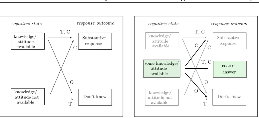
How do respondents typically act in surveys, when they are unable to report one of the provided (categorical) options? In case that “Don’t know” (DK) is admitted as an answer, this option may represent the category of their choice. However, some respondents who could actually give a substantive response might also decide for DK, e.g. to protect private information or to minimize the efforts associated with the memory and decision process, and hence allowing for DK in surveys is debatable. Moreover, there are many cases where respondents are able to exclude several categories and hence their knowledge or attitude is too strong to be best expressed by the DK category. Here, we firstly turn to the principal discussion whether to provide the DK category or not. Afterwards, the idea of offering coarse categories, i.e. options that are not collected in the resolution originally intended in the subject matter context, is embedded as a main proposal of this work in order to maximize the information about the respondents’ opinion.

While most authors (cf., e.g., Gilljam and Granberg, 1993; Krosnick and Presser, 2010; Poe et al., 1988) rather suggest to drop the DK option, there are also some holding the view that the DK option is needed to filter out respondents without real opinion or knowledge on a topic (cf., e.g., Vaillancourt, 1973). Also in more recent research it seems still inadequate to form a clear, general recommendation, since the respondents’ answering behavior, and hence the different drawbacks arising with and without the DK option, may depend on several factors: Examples are the type of the question (like e.g. factual (cf., e.g., Poe et al., 1988) or interpretable question), the topic of the questionnaire (like e.g. sensitive topic or not), the interviewer and the mode of data collection (cf., e.g., Kreuter et al., 2008a).

(18)

response outcome cognitive state

knowledge/ attitude available

available

Substantive response

Don’t know

T, C

T C

O

T, C

T C

O

coarse answer some knowledge/

attitude available

T, C C

O

knowledge/ attitude not

knowledge/ attitude available

cognitive state response outcome

available knowledge/

attitude not Don’t know Substantive response

Figure 1.1: State-response mapping; left: classical model with two states (cf., Beatty and Herrmann, 1995); right: adapted model with the new parts colored.

the judgement with one of the supplied answers (step 4). Furthermore, in case of sensitive questions social desirability (cf., e.g., DeMaio, 1984) may encourage respondents to go for the DK option. Most respondents with the above listed motives for DK are actually able to report a meaningful answer, i.e. an answer that might not be in the required accuracy, but at least bears an increased information compared to DK. For that reason, Krosnick and Presser (2010, p. 285) finally recommend to refrain from an explicit DK category, but to ask follow-up questions that aim at the strength of previously reported attitudes.

An alternative consequence of investigating these reasons – promoted in the present work – is to meet the respondents’ needs by offering different kinds of coarse options, i.e. respondents do no longer have to commit to one single option, but answers as “option a or option b” or scale point “1-3” are acceptable as well. Hence, respondents who have insufficient knowledge to form a judgment in the required accuracy (step 3) or cannot decide between some of the provided answers (step 4) are given the possibility to adequately express their answer. Moreover, respondents refusing to disclose their answer might be prompted to give at least some coarse information instead of DK or a wrong answer.

(19)

3

response outcome by additionally admitting coarse answers (cf. right part of Figure 1.1), which enables respondents with some knowledge to make a truthful statement (T). Some errors remain, when respondents do not confess that they cannot give a substantive re-sponse (C), decide for a wrong (coarse) answer (C) or when there is still no willingness to disclose any information (O). These groups of respondents already existed before, while the related error will be reduced due to the respondents (truthfully) answering with a coarse answer. However, respondents driven by their intuition might give a (correct) substantive report instead of a weak DK in the left model, but decide for a (too) coarse answer in the right model, now where this option is available. To counter this behavior, the choice of a questioning technique that first asks about precise answers, providing coarse answers only in case of a previous nonresponse is recommendable.

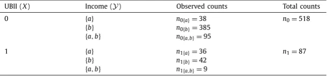
In general, a two-step questioning technique of that kind is employed comparably rarely. However, in the context of the sensitive income question, one sometimes relies on this procedure (cf., e.g., Kennickell, 1996): For example, in the German General Social Survey (cf., GESIS Leibniz Institute for the Social Sciences, 2016) and in the German Panel Study “Labour Market and Social Security” (PASS, cf., Trappmann et al., 2010) income classes are directed to respondents refusing to disclose their precise income. In the latter one, several follow-up questions generate coarse categorical answers with different levels of accuracies. The gain of the explicit collection of coarse answers in the second step becomes directly apparent from Kuha et al. (2017), where initial nonresponders are simply encouraged to give a substantial (precise) response, decreasing (item-)nonresponse bias, but increasing measurement errors. By allowing initial nonresponders to state their answer in their individually required accuracy, measurement errors are expected to be reduced.

To conclude this motivation, we add some general points on coarse data in surveys, also embedding the considerations above. We addressed the quite common situation that the respondents of some survey have to choose between several (categorical) alternatives. In fact, the DK category represents a coarse answer, namely the one where there is no information on specific categories at all. Additionally, the considerations above motivate a more extensive collection of coarse categorical data, recommending that one should not only restrict to the DK option, but also gather coarse answers with different levels of accuracies. Further stressing the gain of information resulting from collecting coarse data by a questioning technique as accomplished by the PASS study and a proper statistical modelling of these data is part of this work.

(20)

(21)

2 Current state of research and aim of

this work

2.1 General literature review and gaps that are filled by

this work

Every analysis of coarse (categorical) data should be preceded by a careful distinction between ontic and epistemic data imprecision (cf., e.g., Couso and Dubois, 2014), because the aim of the analysis and the way to proceed are strongly reliant upon the type of coarse data at hand. The origin of this differentiation can be found in the two interpretations of sets (cf., e.g., Dubois and Prade, 2009):

• On the one hand, a set can be regarded as a collection of elements forming an entity of its own. In thisontic(or conjunctive) view, coarse values, such as_{a, b_}composed of categories aandb, are the precise observation of something imprecise and we refer to data under ontic imprecision in this case. Multiple responses such as the languages one is able to speak (cf., e.g., Couso et al., 2014) or the opinion of partially undecided respondents can be mentioned as examples. In this work, the party affiliation of undecided respondents is studied. In pre-election studies several respondents might be indifferent between some parties in the sense that they themselves do not know which of those parties to elect. Hence, we address imprecise opinions, which can be collected in a precise way.

(22)

While under ontic data imprecision it is of main interest to find a way how the naturally coarse values can be incorporated in the analysis, under epistemic data imprecision one tries to understand the underlying coarsening structure to be able to estimate quantities referring to the latent variable. Due to this implied differentness of the purpose, we now separately review for each type of data imprecision established methods to deal with the respective challenge. Yet, there are a few publications jointly accounting for both types, i.e. uncertain ontic information (cf., e.g., Denœux et al., 2010, by relying on the formalism of belief functions). We set a focus on coarse categorical data and their handling in a survey context and show how our contributions fit into the existing literature.

2.1.1 Ontic data imprecision

The theory of random sets gives a proper framework for the formal representation of the considered kinds of data imprecision, where the respective interpretation of a random set determines the underlying view (cf., e.g., Couso et al., 2014). Although random sets where already indirectly addressed by Kolmogoroff (1933, p. 46) speaking of “a measurable re-gion of the plane whose shape depends on chance”, interest in this topic only increased when Matheron (1975) introduced random closed sets (cf., e.g., Stoyan, 1998) and plenty of applications followed (such as in image analysis, cf., e.g., Molchanov 2004, or in econo-metrics, cf., e.g., Molchanov and Molinari 2014).

Since we restrict to coarse categorical data, studying finite random sets is sufficient, where it is directly visible that random sets can be regarded as generalized random vari-ables, representing a measurable mapping on the power setP(S) instead of the state space

S itself (cf., e.g., Nguyen, 2006). In this way, a finite random set Y is given by

Y : Ω_{→ P}(S), (2.1)

where for the inverse image of each A ⊆ S it has to be valid that Y−1₍_{_A_}_{) =} _{_ω _∈ _{Ω :} Y(ω) = A} ∈ A with (Ω,A) denoting the underlying measurable space (cf., e.g., Nguyen, 2006, p. 35). Understanding a random set as a multiple-valued random variable taking values inP(S) directly complies with the ontic view (cf., Couso and Dubois, 2014), where this formalization serves as a basis in our contribution. Alternatively, data under ontic imprecision can be formally regarded as functional data (cf., e.g., Guillaume and Dubois, 2015, p. 147). Although this is elaborated by Gonz´alez-Rodr´ıguez et al. (2012) for fuzzy data, all results are directly applicable for coarse data, which represent the special case where all subcomponents of our precisely observed imprecise entity are identified with corresponding indicator functions.

Coarse categorical data under ontic imprecision are collected in surveys, whenever re-spondents are given the opportunity to tick more than one of the provided options. In this context, one refers to multiple response data. As illustration we consider the question

Which mediums do you use to be informed about the events of the day? (choose

(23)

2.1 General literature review and gaps that are filled by this work 7

All elements within the power set of the state spaceS =_{newspaper,TV, smartphone app, internet, radio}(one may explicitly exclude the empty set) can then be selected as possible answers, where the answer “_{TV, radio_}” for example is interpreted as own, precisely observed answer expressing that one utilizes TV and radio as channel of information. A consequent analysis should be based on the power set.

While in multi-label classification this is exactly how one deals with multiple responses (cf., e.g., Tsoumakas and Katakis, 2006), in most remaining methods a concrete procedure that gains general acceptance is still missing. Agresti and Liu (1999) (p. 936) recommend to take the contingency table referring to all combinations of answers as a basis, which is equivalent to treating multiple responses as ontic sets, but in many cases the evaluation of multiple response data is still restricted to item specific frequencies (cf., e.g., Santos, 2000). When taking the ontic interpretation of multiple responses seriously, one should calculate frequencies for each combination of items (without order) instead, hence summing up the frequencies of all supersets containing the considered combination (cf., Couso and Dubois, 2014, p. 1505). The frequent ignorance of the nature of multiple responses is even more incomprehensible, when bearing in mind that most statistical software, such as R, SPSS, STATA or SAS, is already able to treat each combination as own category. In this way, statistical software either represents multiple answers as (ontic) sets and/or understands each item as yes (1) / no (0) question (cf., e.g., Koziol and Bilder, 2014). It is obvious that the number of “ontic” categories increases in the cardinality of the state space S and thus can become very large. But specifically in survey questions requiring to tick a specific number of boxes, such as “choose the three most important reasons”, this problem is kept within a limit.

Due to the lack of clear rules how to deal with multiple responses in statistical analyses, in many cases one refrains from providing the “choose all that apply” supplement. One application where this is especially noticeable is given by the question about the voting intention in pre-election studies – at least we did not find any example, where multiple answers were allowed in this context. In this way, this question is frequently asked as follows:

Which of the following parties do you favor?

party A party B party C other party Don’t know

Beyond the problem that there are different reasons prompting respondents to tick the DK category (cf. Section 1), there is a loss of information induced by undecided respondents who are able to exclude specific parties. For that reason, we recommend to add the “choose all that apply” instruction in questions of that kind and then to draw on the formal framework of Couso et al. (2014), interpreting the answers of different groups of “the Undecided” as ontic sets. In our work we also study how to incorporate these multiple responses induced by indecision into commonly used statistical procedures. In doing so, we throughout refer to the application of election studies. For that reason, an overview about common practices in this context is given next.

(24)

voters are able to swing an election (cf., e.g., Gawronski and Galdi, 2011). Thus, it is all the more surprising that characterizing the undecided respondents and investigating how they come to their decision is an understudied topic (cf., e.g., Orriols and Mart´ınez, 2014). In our work, we aim at this goal and try to explain the (coarse) voting intention represented as ontic sets by means of several demographic variables, but also variables related to measures of election campaigns. In this way, we mainly refer to the ontic view, taking the current preferences of the undecided respondents seriously.

However, most political analysts address the epistemic view, studying the final decision when precise voting decisions are made or forced. Since they refrain from explicitly col-lecting the voting intention of undecided voters in most cases, they either base their voting prediction on the decided respondents only or allocate all DK responders to parties in a specific manner (cf., e.g., Bon et al., 2017). Usual ways of allocations are given by even assignments between the major parties or proportional assignments reflecting the voting intention of the decided respondents (cf., e.g., Martin et al., 2005, referred to as “missing (completely) at random” in the missing data literature). Since the answers of the unde-cided and the deunde-cided respondents may substantially differ, a substantial bias is expected for the voting prediction. More sophisticated, but rarely applied allocations of “Unde-cided” include imputation-based (cf., Fenwick et al., 1982) and Bayesian assignments both making use of information about other variables, while the latter one additionally exploits prior information about voting for each specific party (cf., Press and Yang, 1974). Even though these approaches account for some available information about the undecided re-spondents, an adequate understanding of uncertainty in prediction models is still missing (cf., e.g., Rothschild, 2015). However, in some cases the uncertain behavior of voters is at least captured in the data collection process. In this way, verbal statements, such as “Lean towards party A”, or probabilistic votes , quantifying the degree of certitude in the party preference, are offered (cf., Burden, 1997; Delavande and Manski, 2010).

AlthoughContribution 1, which addresses this topic, mainly refers to ontic data impre-cision, it also suggests an interval-valued prediction reflecting the underlying uncertainty. This is in accordance with the conception of epistemic data imprecision used in the re-maining contributions. A corresponding literature review is given next.

2.1.2 Epistemic data imprecision

Coming back to the definition of a random set given in Equation (2.1), apart from its ontic interpretation applied in Section 2.1.1 there is also an epistemic one: Instead of considering a random set as a multiple-valued random variable on P(S), we can also understand it as a multiple-valued mappingYepist: Ω→ P(S) representing the disjunctive set of precise

random variables Yprecise : Ω→S (cf., Couso and Dubois, 2014) that are compatible with

the (incomplete) realizations of Yepist and are often called selections. Hence, when taking

the epistemic view, we interpret the random set as

(25)

In our contributions concerning epistemic data imprecision (i.e. in Contribution 2 to Con-tribution 5), the random variable Y, which refers to the true underlying construct, has a key role. In this way, Y denotes a specific selection Yprecise, when regarding the epistemic

interpretation of a random set. Statistical inference about the distribution of Y repre-sents our main interest, where maximum likelihood estimation is used as an estimation technique.

SinceYepistis regarded as the collection of several precise models that can be inferred from

the incomplete knowledge, point-identification of the distribution of Y is only guaranteed in special cases. Point-identification is a general property meaning that different values of parameters have to induce different probability distributions of the considered random variables (cf., e.g., Lehmann and Casella, 2006, p. 24). To ensure point-identification, classical statistics mostly breaks down the problem by including technical restrictions that are strong enough to point-identify the parameters of interest. In this way, in the context of coarse data strict assumptions on the coarsening process are incorporated. The origin of these assumptions and also of most approaches dealing with coarse data lies in the area of missing data. For that reason, commonly used approaches for missing data are presented first, then proceeding to the situation of coarse data beyond the missing case.

Current methods for dealing with missing data

In the missing data literature1 _{the differentiation between various} _{types of missingness} mechanisms, i.e. “missing completely at random” (MCAR), “missing at random” (MAR) and “missing not at random” (MNAR), is essential. While the missingness is independent of the observed and the missing values under MCAR, under MAR it is dependent on the observed values and under MNAR even on the actual missing values (cf., e.g., Little and Rubin, 2014). In the context of likelihood inference, MCAR and MAR (plus parameter distinctness, cf., Little and Rubin 2014, p. 119) are especially desirable, since under these assumptions the complete-data likelihood is proportional to the likelihood ignoring the missingness mechanism (cf., Little and Rubin, 2014, p. 119), whose parameters are point-identified. However, it is important to be aware of the fact that the correct assumption about the true underlying mechanism is a necessary prerequisite to receive unbiased esti-mators. This point turns out to be a major difficulty, since testing of missingness assump-tions is generally impossible (cf., e.g., Manski, 2003, p. 26). Hence, it is problematic that widespread techniques dealing with missing data, such as imputation or the EM-algorithm, are based upon the MAR assumption (cf., e.g., Jaeger, 2006). Moreover, complete-case and available-case analyses completely ignoring the missingness are still quite common (cf., e.g., Geva et al., 2013; Rombach et al., 2016).

Imputation methods aim at valid statistical inferences by replacing missing values by plausible ones. For this purpose, the imputed values are derived from a predictive distribution described by the observed values, where the way of drawing from this distri-bution varies for the different imputation methods, such as mean imputation, regression

(26)

imputation or hot-deck imputation (cf., e.g., Weisberg, 2009). Recent examples recom-mending multiple imputation in a survey context are given in Pampaka et al. (2016), who refer to a case study with educational data, as well as Frick and Grabka (2014) and Spieß (2009) discussing this method for the data of the German Socio-Economic Panel (SOEP). The EM algorithm (cf., Dempster and Laird, 1977) is likelihood-based iterative pro-cedure that relies on starting values for the parameters of interest and then determines the expectation of the joint distribution (complete-data likelihood) given the observation. This expectation provides the basis for re-estimating the parameters of interest, while this procedure then continues until some stability is achieved (cf., e.g., Schafer, 1997). Both, methodological reviews about dealing with missing data (cf., e.g., Dong and Peng, 2013) and practical applications (cf., e.g., Kariuki et al., 2015) include the EM-algorithm as a standard method.

Although one mostly sticks to the already mentioned procedures, there are also a few

approaches that explicitly refrain from the MAR assumption and intend to model the

underlying missingness process instead. In this way, selection models split the joint distribution2 _{of the missingness variable}3 _M _{and the variable} _Y _{into one part referring to}

Y (outcome model) and one part referring to M given the variable Y (generally called

selection model, but here missingness model to distinguish it from the general term) (cf., e.g., Toutenburg et al., 2004). Choosing the missingness model represents a crucial difficulty of this procedure. A specific, popular variant of the selection model is the Heckman selection model (cf., Heckman, 1979), combining an outcome model and a missingness model as follows: Based on the assumption of a multivariate normal distribution, the correlation between the error terms of the two model equations is explicitly included. The selection bias is then fully traced back to this correlation and used to correct the estimators obtained under MAR (cf., e.g., Amemiya, 1985, for more details). Beyond the problem of imposed distributional assumptions, – as in the general selection model– finding variables that appropriately explain the missingness process definitely stays a challenging and mostly impossible task.

For that reason, asystematic sensitivity analysisis performed in some cases, regard-ing different missregard-ingness models that impose various, from a practical viewpoint conceiv-able missingness assumptions. Each (specific) precise missingness model point-identifies the distribution of Y, wherefore the parameter specifying the missingess process can be regarded as a kind of nuisance parameter, also called sensitivity parameter in this context (cf., e.g., Kenward et al., 2001). Considering the whole range of results inferred from dif-ferent, reasonable missingness models, then gives a set-valued estimator of the distribution of Y. In this way, the idea of a systematic sensitivity analysis differs from a conventional sensitivity analysis (as e.g. performed in Goldsmith, 2005) simply investigating the impact of a deviation from the imposed assumptions without understanding it as a part of the result. Examples of a systematic sensitivity analysis in a categorical setting are given in

2_{This joint distribution corresponds to the complete-data likelihood.}

(27)

Baker et al. (1992), Kenward et al. (2001) Molenberghs et al. (1999), Molenberghs et al. (2001) and Nordheim (1984), where in the context of regression this topic is raised by Baker and Laird (1988) and Moreno-Betancur et al. (2015). Strongly related to selection models are pattern-mixture models. In pattern-mixture models one factorizes the joint distribution of Y and M in the opposite way, hence regarding the marginal distribution of M and the distribution of Y given M (cf., e.g., Little, 1993), where again systematic sensitivity analyses show to be beneficial (cf., e.g., Daniels and Hogan, 2000). However, in most contributions and also throughout this work, the representation of a selection model is used.

The idea of the methodology ofpartial identification(cf., e.g., Manski, 2003) resembles the one of systematic sensitivity analyses, except for proceeding in the opposite direction: While the collection of all results obtained under plausible assumptions about the missing-ness process is taken if a systematic sensitivity analysis is performed, partial identification starts by making no assumptions on the missingness process at all, but then successively includes all available, (weak) auxiliary information that is frequently not strong enough to ensure point-identification. This careful inclusion of auxiliary information about the missingness gradually refines the result in such a manner that imprecision is reduced, but does not disappear, except sufficient information was available (cf., e.g., Manski, 2005a). Thus, by admitting the possibility that parameters are partially identified, identification does no longer have to be taken as a binary concept in the sense that parameters are either identified or not (cf., e.g., Tamer, 2010). Practical examples for the inclusion of auxiliary information are for instance given in Jiang and Ding (2016).

Manski’s original application of partial identification addresses the selection problem arising when the estimation of treatment effects on outcomes is the main goal (cf., e.g., Manski, 1989, 1990, 2003, 2005b; Stoye, 2009), such as the influence of the family structure on children’s outcomes (cf., Manski, 1999). In this context, only tenable assumptions on the so-called counterfactuals (“what-if probabilities”) are imposed (cf., e.g., Morgan and Winship, 2014, for more details about causal inference in general). Furthermore, areas forcing point-identification by strong, and sometimes questionable assumptions may profit from the underlying idea. Examples are given in Di Zio and Vantaggi (2017), Molinari (2008), K¨uchenhoff et al. (2012) and Tamer (2010), who exploit partial identification in statistical matching, misclassification and more general in econometrics.

(28)

Current methods for dealing with coarse data

Analogously as in the missing data situation, considering the likelihood under coarse data may lead us to the following question: “Which conditions allow a simplification of the complete-data likelihood in the sense that the coarsening can be ignored?” This question is

answered by Heitjan and Rubin (1991) requiring parameter distinctness and “coarsening

at random” (CAR). In their definition of CAR they postulate that the probability of each fixed (coarse) observation does not depend on the true underlying value, as long as this value is consistent with the observation. In Jaeger (2005b) this assumption is called distributional CAR (d-car) and is distinguished from theG-carvariant by Heitjan (1997), which gives a more direct extension of MAR by relying on a representation in terms of the coarsening variable G. This variable G is a generalization of M, not only differentiating between observed and missing values, but between several degrees of coarseness. Whenever asymmetric, mixture or probabilistic rounding/heaping is present (cf., e.g., Schneeweiß et al., 2010), the formalization of a coarsening variableG is widely spread. In these cases, one either models the rounding by the exceedance of certain thresholds of G (cf., e.g. Drechsler et al., 2015; Heitjan and Rubin, 1991, Example 2) or by a so-called rounding profile function (cf., e.g. Torelli and Trivellato, 1993; Schneeweiß and Komlos, 2009), e.g. in dependence of the interval width. Taking the rounding process into account in this way and relying on certain smoothness conditions (cf., Kendall, 1938), the estimation of the variable of interest’s mean is nearly unbiased, while the variance can be adjusted by the Sheppard’s correction (cf., Sheppard, 1897) extended in Schneeweiß and Komlos (2009) for cases beyond simple rounding. However, although one explicitly decides to model the rounding process, in most cases the rounding is assumed to be independent on the true underlying value, in the sense that one relies on the G-car assumption. Like most of the papers, this work also refers to the CAR variant as formulated by Heitjan and Rubin (1991), which is less restrictive compared to G-car (cf., Jaeger, 2005b). Nevertheless, the MCAR analogue for coarse data, i.e. “coarsening completely at random” (CCAR), is only

reasonable when presented in terms of a variable G. Like G-car, CCAR requests the

distribution ofG to be independent of the true value, but now one refrains from requiring that this true value has to be consistent with the observation (cf. Heitjan 1994).

Another assumption that expresses a kind of lack of information about the observation process is the superset assumption (cf., e.g., Couso and Dubois, 2018; H¨ullermeier and Cheng, 2015). It resembles the original CAR assumption, but switches the values that are held fixed. Hence, the probability of an observation given a fixed, true, underlying value is assumed to be constant for each observation that is compatible with this true value (cf., Couso and Dubois, 2018). In the context of updating probability distributions (cf., e.g., Gr¨unwald and Halpern, 2003), the CAR assumption4 _{naturally arises in a reverse}5 _form (also called RCAR) (cf., Theorem 10 in van Ommen et al., 2016). In this context, the RCAR condition is not an assumption, but is rather obtained as a result whenever one pursues a minimax strategy (cf., Section 2.1 in van Ommen et al., 2016).

(29)

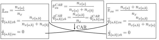
In this work, the CAR assumption is considered in a regression context and hence it is additionally conditioned on the values of the covariates. This assumption corresponds to the conventional assumption made in survival analysis that conditional on some covari-ates the censoring time is independent of the survival time. This is often referred to as “independent censoring”. Since the estimators of survival rates may be biased whenever independent censoring is wrongly assumed (cf., e.g., Zheng and Klein, 1995), frameworks were developed that rely on dependent censoring, such as the copula-based approaches by

Huang and Zhang (2008) and Emura and Chen (2016). Moreover, in Contribution 2 a

new coarsening assumption called subgroup independence (SI) is introduced: While under

CAR the coarsening is independent of the values of Y, but dependent on the covariate

values, the (in)dependence structure under SI is the other way around. We do not only study maximum likelihood estimation under these assumptions, but also investigate the (im)possibility of testing these assumptions. Although CAR is generally impossible to test, some hypothesis tests have been suggested in the literature, all relying on strong assumptions: For instance, testability of CAR can be achieved under the availability of in-strumental variables and bounded completeness (cf., Breunig, 2017) or when distributional constraints on the structure of a network are incorporated (cf., Jaeger, 2006). Generally, the challenge remains to distinguish between situations where CAR is justifiably rejected or not rejected and situations where the test decision is meaningless, since the included additional assumptions were wrongly made.

Commonly used approaches for missing data have been extended for coarse data, such as imputation (cf., e.g., Heitjan and Rubin, 1990; Kim and Hong, 2012) and the EM-algorithm. While both imputation and the EM-algorithm are always reliant upon the quite restrictive CAR assumption (cf., e.g., Jaeger, 2006), the latter one was additionally investigated to be reasonable only in situations where the coarse observation of each true value is predetermined, as e.g. satisfied in case of grouped data (cf., Couso and Dubois, 2016). Since the EM-algorithm is likelihood-based as our approach, a more detailed com-parison of the respective results is of interest. We postpone this purpose to Section 3.2.4, where all necessary notations already have been clarified. In this connection we will also contrast our idea to that of other likelihood-based ideas, relying on different optimization strategies, such as the minimax (cf., e.g., Guillaume and Dubois, 2015) or the maximax (cf., e.g., H¨ullermeier 2014) approach. Jaeger (2016) presents an algorithm whose underlying idea resembles the maximax strategy: His AI & M (adjusting imputation and maximiza-tion) procedure explicitly refrains from concrete coarsening assumptions, but relies on the view that given the data some mechanisms appear to be more likely than others.

Imposing the CAR assumption or making use of specific optimization strategies to force point-identified parameters is not always justified. For that reason, there are some

ap-proaches that only includeweak or even no assumptionsabout the coarsening process.

(30)

vari-able and categorical precisely observed covariates. A general framework for learning from coarse data is given in Couso and S´anchez (2016) and S´anchez and Couso (2018).

There are also Bayesian approaches, describing information about the coarsening

process via corresponding prior assumptions. An example is given in Zaffalon and Miranda (2009): Just as our approach, their conservative inference rule (CIR) aims at refining the result under total ignorance of the missingness/coarsening assumption, where it practically coincides with the conservative updating rule presented in De Cooman and Zaffalon (2004). By applying CIR, a compromise between a too optimistic and too pessimistic knowledge about the missingness/coarsening process is given, assuming CAR in the context of some variables and total ignorance about the coarsening process of other variables. Our approach does not force us to decide for one extreme case, i.e. either no or complete knowledge about the coarsening, but allows us to incorporate (arbitrary) weak coarsening assumptions in a careful way. For instance, the coarsening probability can be assumed to be higher for specific groups of respondents compared to others. The inclusion of such auxiliary information is an important part of our contribution (cf. Section 3.2.1 and the summary of Contribution 2 in Section 3.2.3).

2.2 Aim of this work

This section is closed by briefly outlining the highlights of this work. This PhD thesis aims at providing ways for a natural inclusion of all tenable information about the coarse structure of the data into commonly used statistical models. In particular, we promote. . .

• . . . the explicit differentiation between epistemic and ontic data imprecision in data

collection as well as in data analysis.

• . . . the explicit collection of coarse categorical data: We allow “the Undecided” to

report multiple answers and give respondents with insufficient knowledge in the topic of the question or poor willingness to disclose their answer the opportunity to give coarse answers. This can also be regarded as a possible strategy to minimize the errors arising in the four cognitive states of respondents when answering survey questions (cf. Section 1).

• . . .a medium to regulate the inclusion of auxiliary information, which allows to

incor-porate subject-driven coarsening assumptions instead of strong, untestable ones, such as CAR. In this way, auxiliary information about the coarsening process that is not sufficient to point-identify the parameters of interest can now explicitly be exploited, while it would have to be left out of consideration under traditional approaches.

• . . . a new coarsening assumption called subgroup independence, which is indeed

testable in specific settings. A hypothesis test for SI is proposed.

(31)

3 About the contributing material:

Relations, summaries and outlooks

In this chapter we take a closer look at the papers contributing to this thesis. All the contributions address methods for carefully handling coarse data exploiting all available information about the coarse structure of the data. When referring to ontic data impre-cision, i.e. in Contribution 1, this goal is reflected by explicitly collecting coarse data and taking its coarse nature seriously in the analysis, while under epistemic data imprecision, i.e. in Contribution 2 to 5, only tenable assumptions about the coarsening process are

contemplated. To some extent, Contribution 1 addresses epistemic data imprecision as

well: In this case, interval-valued forecasts are suggested by relying on Dempster’s lower and upper probability (cf., Dempster, 1967). When no assumptions about the “decision process” are included, these intervals are in line with the ones obtained from the framework used in the contributions referring to epistemic imprecision. Under the availability of some auxiliary information, such as “undecided respondents rather vote for the SPD compared to the Green party”, the interval-valued forecasts may profit from the estimation framework developed in Contribution 2.

This chapter is again structured by the respective type of data imprecision (cf. Section 3.1 for the ontic and Section 3.2 for the epistemic case). Both parts give an overview of the corresponding contributions followed by some remarks and ideas for future research. Since the contributions referring to epistemic data imprecision are built upon a joint basis, it is reasonable to start the associated part more generally by presenting this common ground as well as interrelations between the included contributions.

3.1 Ontic data imprecision: Contribution 1

3.1.1 Summary

(32)

ruled out, when a state space S = _{a, b, c, d_} is underlying. As if this wasn’t enough, frequently the analysis is based on the decided respondents only, which – due to a potential systematic difference between decided and undecided respondents – may provoke biased results (cf., e.g., Bon et al., 2017).

Allowing for multiple answers and regarding them as categories of their own gives a way out of the explained dilemma: One not only respects the heterogeneity in the group of undecided respondents, but even reflects the opinion of the respondents in the most informative way. More formally, this corresponds to reinterpreting a random conjunctive set (cf., Couso and Dubois, 2014), defined as a measurable mapping into the power set, as precise random object (cf. Section 2.1.1, in particular Equation (2.1)). Hence, one simply needs to extend the original state spaceS of our variable of interest to the power set of S

(without the empty set) to account for ontic data imprecision. Relying on this new state space S∗ ₌_P₍_S₎_{\ {∅}} _{is the only thing that changes, while the statistical methods stay} the same. We stress this point by elaborating the idea for the multinomial logit model and classification trees. In case of the multinomial logit model with ontic data imprecision in the response variable, the power-set based analysis not only gives us category specific regression coefficients for each precise, but also for each coarse category, perfectly representing the conception of understanding different types of undecided respondents as groups of their own. In the context of classification (trees), relying on a class variable with values withinS∗ instead of S already represents a comparatively well-established procedure, then referred to as multi-label classification (cf., e.g., Tsoumakas and Katakis, 2006).

Illustrating the ontic approach faces us with new challanges: As far as we know, there is not any pre-election study that allows undecided respondents to express their voting intention by multiple answers. The “German Longitudinal Election Study (GLES) 2013” (cf., Rattinger et al., 2014) at least collects some information on the certainty of the vot-ing intention as well as the assessment of several parties, along with the current, precise (and thus partly forced) voting intention. This gives us the opportunity to construct a new variable “ontic” (cf. Table 1 of Contribution 1 and corresponding explanations), partly consisting of multiple answers, which reflect the respondent’s indecision. In this way, we can compare the obtained results based on this new variable with the ones from a traditional analysis, only including answers of decided respondents. The regression esti-mates from the multinomial logit model in both analyses indicate remarkable differences (cf. Table 4 of Contribution 1), partly even connected with a change in sign. Due to the underrepresentation of undecided respondents induced by the underlying sampling design, the results are even expected to differ to a higher extent. Moreover, the general reduction of the sample size in the course of the construction of the ontic variable might cause to vanish the significance of some estimators.

(33)

3.1 Ontic data imprecision: Contribution 1 17

is getting more and more important, because an increasing number of voters make their vote decision shortly before the election day (cf., e.g., Dassonneville, 2016). The transfer to S∗ _{may substantially increase the computational complexity, but by restricting to the} most important groups, e.g. determined via substance matter reasons (indecision between certain parties is more likely compared to others) or regularization techniques, one can cope with this difficulty.

Furthermore, we calculate interval-valued forecasts, which demands to change the under-lying perspective in the sense that we make an epistemic reinterpretation of the data (also underlyingContribution 2 to 5, summarized in Section 3.2.3): In the election example, we assume that the election day has come, forcing the respondents to make a decision. Using the GLES’13 data to forecast the proportion of respondents electing a specific party, we now understand coarse answers no longer as entity of their own, but as incomplete know-ledge. We formally anchor this idea by relying on the notion of ill-known random variables (cf. Equation (2.2)), hence considering several precise models that – due to this incomplete knowledge – cannot be distinguished (cf., Couso and Dubois, 2014), which then gives us proper interval-valued forecasts (cf. p. 265 of Contribution 1).

3.1.2 Comments and perspectives

The framework presented in Contribution 1 can be adapted for several modifications of

the setting addressed there. Not only extensions to various categorical regression models besides the multinomial logit model, but also to coarse ordinal response variables are straightforward. In this section, apart from a brief motivation and some considerations with regard to these points, also first results from a recent study providing multiple responses are given. In this way, one is able to evaluate the suggested new formulation of the question without being forced to rely on a artificially constructed variable “ontic”.

More general discrete choice models

In our application example we used the multinomial logit model, which only represents one specification of a variety of discrete choice models (cf., e.g., Train, 2009, to get an overview). While the multinomial logit model is restricted to describe the voting intention by voter characteristics, the conditional logit model introduced by McFadden (1973) shows a linear predictor that is limited to account for the party attributes as perceived by the voter, mostly relying on the ideological distance between the party and the voter (concerning different issues, such as environment or taxes etc.) (cf., e.g., Alvarez and Nagler, 1998). In current practices of voting research more flexible modelling approaches are favored that combine both model specifications, thus considering the linear predictor (cf., e.g., Dow and Endersby, 2004)

ηij =xi·βj+zij ·γ , (3.1)

(34)

party specific coefficientsβj are included, while the covariates xi are constant across party

choices. The idea of the conditional logit model is expressed by the second component of the sum in (3.1), where a global regression coefficientγand voter characteristicszij varying

through party choices are incorporated.

Due to the general character of our idea to deal with “the Undecided”, we can directly apply the ontic approach to the combined model with the linear predictor in (3.1). Apart from the adaption of the state space S to S∗_{, nothing has to be changed. Just like in the} multinomial logit model, party-specific regression coefficientsβj for all groups of undecided

respondents are a direct consequence of this adaption. Since the coefficients γ from the conditional logit model component in (3.1) are global, no additional modifications are needed here.

Coarse ordinal data

So far, we addressed a coarse categorical response variable of nominal scale. However, the phenomenon of indecision may also arise in connection of variables showing an ordinal scale of measurement. Considering rating scales, there are different possibilities to deal with indecision. Some surveys provide a DK or “Undecided” category additionally to the rating scale; consequences of this procedure have already been discussed in Section 1 and Section 2.1.1. Whenever an additional category of that kind is omitted, the behavior of “the Undecided” is guided by the number of response categories: Offering an even number of response categories forces undecided respondents to a decision, while an odd number prompts them to choose the midpoint of the scale. One generally detects a “tendency to the middle” (cf., e.g., Friedman and Amoo, 1999), which is undesirable, since the meaning of the middle category as “neutral response” might be distorted by comprising e.g. undecided and satisficing respondents as well as respondents avoiding social embarrassment (cf., e.g., Sturgis et al., 2014).

Against this background, Iannario and Piccolo (2011) and others consider the CUB model1_{. The core of this approach is the distinction between the attractiveness towards} the item (also called feeling) and fuzzyness around the final choice (also referred to as uncertainty). While the feeling is traced back to several individual characteristics such as age or previous experience, the uncertainty component is determined by circumstances as tiredness, time devoted to the question or the incentive to satisfice. The final CUB model is then composed as a mixture of the feeling and the uncertainty component. In this way, the CUB model deals with the “tendency to the middle” problem by an explicit inclusion of a random variableU describing confounding factors, called “uncertainty”. The original model represents the special case where any “tendency to the middle” is neglected, just utilizing U _{∼ U}(1, k) (with_U representing the uniform distribution) and hence attributing a constant probability to each of the alternatives 1, . . . , k. A proposal to explicitly reflect the “tendency to the middle” is given in Tutz and Schneider (2017): There a beta-binomial distribution is assumed for the uncertainty, i.e. U _∼ BetaBinom(k, α, β) with α, β > 0,

(35)

3.1 Ontic data imprecision: Contribution 1 19

whereα=βis throughout assumed. The parameterαdetermines the concentration of the distribution in the middle and is explicitly modelled by the covariates used in the model for the feeling component.

By allowing for multiple answers and then relying on the ontic view, the problem of a proper description of the uncertainty component could be avoided. Again, an extension of the state space represents the crucial adaption. However, this may bear the challenge of analyzing partially ordered (cf., e.g., Schollmeyer (2017a) for descriptive analyses or Schollmeyer et al. (2017) with regard to stochastic dominance) coarse data: Considering different levels of undecided respondents, such as {3,4} and {3,4,5} when referring to a rating scale, expresses a clear ordering between some categories (e.g., _{3,4_} < _{3,4,5_}), while leaving it open for others (e.g. {3,4,5} Q {4}). By referring to regression analysis, a first idea for dealing with this problem is given: A commonly applied model for ordinal responses is the cumulative logit model (cf., e.g. Fahrmeir et al., 2013, p. 334–337). It relies on the proportional odds assumption, which requires global regression coefficients, and hence no own regression estimators have to be estimated for each coarse category (just as in the conditional logit model, see above). The model reflects the (strict) ordinal structure by additional restrictions on the category-specific intercept β0r, r ∈ {1, . . . , k},

assuming

β01 < β02 < . . . < β0k

for the k ordered categories (cf., e.g. Fahrmeir et al., 2013, p. 336). As a direct con-sequence of the partially ordered structure implied by the “ontic” variable, restrictions between incomparable categories have to be omitted. This should correspond to a proce-dure that repeatedly estimates regression coefficients based on a cumulative logit model, but varies between all conceivable orders of the category-specific intercepts. Those regres-sion estimators that achieve the maximum value of the likelihood are then finally taken. Further research should be devoted to this, here only briefly discussed, problem, also ex-ploiting findings from already existing literature about categorical regression with partially ordered response variables (cf., e.g., Zhang and Ip, 2012). Considering party preferences on a left-right continuum and hence applying ordinal models as suggested above in this context as well, gives us results about the placement of several coarse party preferences on the left-right continuum as a by-product.

Gain of information induced by the new voting question

(36)

AfD CD CD-AfD CD-FDP CD-SPD FDP

40 90 10 12 21 26

Green Left SPD SPD-Green DK _≤10 supporters

99 38 78 21 91 84

Table 3.1: Group 2: Absolute frequencies of party affiliations. The delimiter “-” separates the parties between which respondents are undecided.

jointly conducted by the University of Mannheim and the Institute for Employment Re-search, Nuremberg (cf., Horwitz et al., 2017). A split ballot experiment was used: One half of the respondents was asked to choose a single party (group 1), the other half was given a multiple choice option (group 2). Since the respondents were randomly assigned to the type of question and both groups show large sample sizes (n = 611 respondents could choose one party only, while n = 610 were allowed to decide for multiple parties), it is justified to assume that similar true voting intentions are underlying in both groups.

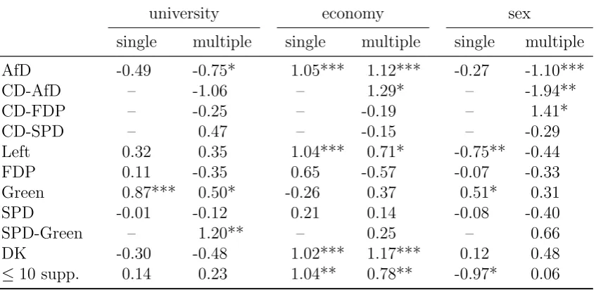
The reduction of the DK proportion induced by the multiple-choice option is (notably) visible: While 18.8% chose DK within group 1, a respective proportion between 14.9% (when restricting to DKs as a single answer) and 16.1% (when additionally considering all supersets) is determined based on the data of group 2. Due to the non-neglectable amount of respondents who decided for multiple parties in group 2 (133 of 610 respondents), it additionally appears that several respondents in group 1 felt forced to give a single option. In a first illustrative study, we compare the regression estimators obtained from a multi-nomial logit model separately applied for both groups (similarly as in Contribution 1). The party affiliation is taken as response variable, in group 1 with single responses only and in group 2 with multiple responses as given in Table 3.1. To avoid that the regres-sion estimators are calculated based on a small number of respondents only, we restrict to the party affiliations that were reported by at least ten respondents and summarize the remaining ones in a joint category (called “less than 10 supporters”)2_{. The variables} “university entrance” (abbreviated by university, with values “no” (=reference category (ref)) and “yes”), sex (with values “male” (ref) and “female”) and the dichotomized per-sonal assessment of the general economic situation (abbreviated by economy, with values “very good or good” (ref) as well as “fairly, bad or very bad”) are used as covariates. In both analyses, we choose “CDU/CSU” (abbreviated by CD for Christian Democrats) as a reference category, which is – according to corresponding3 _{pre-election studies (cf., e.g.,} infratest dimap, 2016) – the most popular party.

In Table 3.2 some results are presented. Most regression estimators are remarkably differ-ent in both analyses, in some cases even connected with changes in sign (cf., e.g., estimator for Green/economy or FDP/economy). Moreover, some significant regression coefficients