String Backgrounds
String Backgrounds
Dissertation
der Fakult¨
at f¨
ur Physik
der Ludwig–Maximilians–Universit¨
at
M¨
unchen
vorgelegt von
J¨
org Michael Fuchs
Stuttgart
Zweitgutachter: Prof. Dr. Dieter L¨
ust
Datum der Abgabe: 8. Juni 2017
Zusammenfassung vii
Abstract vii
1 Introduction 1
2 Conformal field theories of Calabi-Yau compactifications 9
2.1 IIB string theory on Calabi-Yau threefolds . . . 10
2.2 Conformal field theory . . . 13
2.3 Simple currents . . . 23
2.4 N = 2 superconformal field theories . . . 28
2.5 Landau-Ginzburg model . . . 32
2.6 The geometry of Landau-Ginzburg models . . . 38
2.7 Hodge numbers of Calabi-Yau manifolds . . . 44
2.8 Gepner models . . . 48
3 Conformal field theories for non-geometric backgrounds 55 3.1 Linking gauged supergravities and (asymmetric) toroidal orbifolds . . . 56
3.2 Asymmetric Gepner models with N = 1 supersymmetry . . . 59
3.3 Partial supersymmetry breaking ofN = 2 gauged supergravity . . . 64
3.4 Comparison of ACFTs and GSUGRA . . . 71
4 Asymmetric Gepner models with extended supersymmetry 73 4.1 Super-Higgs effect . . . 74
4.2 Classification scheme and the CFT setup . . . 75
4.3 ACFTs inD = 8 . . . 76
4.4 ACFTs inD = 6 . . . 79
4.5 ACFTs inD = 4 . . . 83
4.6 Conclusion . . . 88
5 Gravity in the non-associative R-flux space 91 5.1 The R-flux star product . . . 92
5.2 Symmetries in presence of a star product . . . 96
5.4 Working with the full phase space . . . 110
5.5 Tensor calculus . . . 114
5.6 Differential geometry . . . 117
5.7 Scalar products and the metric . . . 122
5.8 A glimpse at a star Einstein-Hilbert action . . . 125
5.9 Conclusion . . . 126
A Details about the computer program 127 A.1 Object oriented structure of the program . . . 127
A.2 Performance and other issues . . . 134
B Supermultiplets 137 B.1 Supergravity in D= 8 . . . 137
B.2 Supergravity in D= 6 . . . 140
B.3 Supergravity in D= 4 . . . 142
C Computing the star Riemann tensor 145
Diese Doktorarbeit diskutiert zwei Aspekte von nicht-geometrischen Stringhintergr¨unden, welche durch links-rechts asymmetrische konforme Feldtheorien definiert sind.
Mithilfe von simple currents werden vierdimensionale links-rechts asymmetrische Typ IIB Gepnermodelle mit N = 1 Supersymmetrie konstruiert. Die Analyse der masselosen Vektormultiplets weist die Kombinatorik einer zugrundeliegenden complete intersection Calabi-Yau-Mannigfaltigkeit auf. Diese Beobachtung legt nahe, dass diese asymmetrischen Gepnermodelle einem voll r¨uckgekoppeltenN = 1 Vakuum in der geeichten N = 2 Super-gravitationstheorie entsprechen, welche man durch eine Flusskompaktifizierung von Typ IIB auf der zugrundeliegenden Calabi-Yau-Mannigfaltigkeit erh¨alt. Wir verifizieren diese Hypothese, indem wir das Spektrum von mehreren asymmetrischen Gepnermodellen mit den notwendigen Bedingungen vergleichen, welche beim Brechen von N = 2 → N = 1 in der geeichten Supergravitationstheorie existieren. Um weitere Beweise f¨ur die ver-mutete Korrespondenz zwischen asymmetrischen konformen Feldtheorien und geeichten Supergravitationstheorien zu finden, werden mithilfe einer stochastischen Computersuche s¨amtliche links-rechts asymmetrische Gepnermodelle in vier, sechs und acht Dimensionen mit mindestens acht Superladungen klassifiziert. Alle Modelle k¨onnen wenigen verschiede-nen Klassen zugeordnet werden, welche sich durch dimensionale Reduktion, asymmetrische Orbifolds mit (−1)FLDivisor, Eicherweiterung und, am wichtigsten, den super-Higgs Effekt
erkl¨aren lassen. Die Gepnermodelle in letzterer Klasse zeigen dabei die charakteristischen Merkmale einer gebrochenen geeichten Supergravitationstheorie.
Der zweite Teil der Doktorarbeit widmet sich dem nicht-assoziativen Sternprodukt, welches f¨ur nicht-geometrische R-Fluss Hintergr¨unde auftreten soll. Da das Sternprodukt im Sektor der geschlossenen Strings auftritt, gab es in letzter Zeit Bem¨uhungen, die Dif-feomorphismensymmetrie der Stringtheorie mit dem Sternprodukt in Einklang zu bringen. In der mathematischen Literatur wurden schon erfolgreich Sternverallgemeinerungen von Tensoren, Zusammenh¨angen und der Riemann Kr¨ummung konstruiert. Wir f¨uhren diese Bem¨uhungen fort, indem wir mehrere L¨ucken f¨ullen und zum Beispiel die Torsion, eine Metrik und ihr Sterninverses definieren. Wenn es darum geht, eine Metrik zu definieren, begegnen wir großen Schwierigkeiten, welche man allesamt auf die nicht-Assoziativit¨at des Sternproduktes zur¨uckf¨uhren kann.
This PhD thesis will discuss two aspects of non-geometric string backgrounds defined by left-right asymmetric conformal field theories.
Using simple currents we construct four-dimensional left-right asymmetric Gepner mod-els of type IIB with N = 1 spacetime supersymmetry. An analysis of the massless vector multiplets reveals the combinatorics of an underlying complete intersection Calabi-Yau. This observation suggests that these asymmetric Gepner models might correspond to a fully backreacted N = 1 vacuum in the N = 2 gauged supergravity, which is the effective action of the type IIB flux compactification on the underlying Calabi-Yau manifold. We check this conjecture by comparing the spectrum of several asymmetric Gepner models with the necessary conditions for an N = 2 → N = 1 breaking in the associated gauged supergravity. To provide further evidence for the conjectured correspondence between asymmetric CFTs and gauged supergravities, we classify left-right asymmetric Gepner models in four, six and eight dimensions with at least eight supercharges using a stochastic computer search. We can sort all models into few different classes that can be explained as dimensional reductions, asymmetric orbifolds with an (−1)FL factor, gauge enhancement
and, most importantly, the super-Higgs effect. The asymmetric Gepner models in the latter class exhibit the characteristic features that are expected from a gauged supergravity.
The second part of this thesis deals with the non-associative star product that is sup-posed to appear in presence of a non-geometric R-flux. Since the star product appears in the closed string sector there have been recent attempts to reconcile the diffeomorphism symmetry of string theory with the star product. In the existing mathematical literature were able to construct star generalizations to tensors, connections and the Riemann cur-vature. We continue these efforts by filling several gaps like introducing a torsion, a metric and its star inverse. When it comes to the metric we encounter major obstacles that can be traced back to the non-associativity of the star product.
Introduction
For centuries physics have followed a simple but extremely successful pattern: Empiric experiments yielded ever new results, which then had to be explained and put into a consistent mathematical theory. However, since the 20th century mathematical knowledge has increased to such an extent that the traditional order, theory follows experiment, has been turned around in not just a few cases. One of the major examples for such a turnaround is probably Albert Einstein, who found his theory of general relativity by relying solely on gedankenexperiments and mathematical reasoning, rather than specific experiments. Only afterwards his theory was experimentally confirmed to be superior to Newton’s law of gravity. Another famous example is the anticipation of the antiparticle of the electron by Paul Dirac, found four years later or the prediction of the neutrino by Wolfgang Pauli. Nowadays particle physicists have agreed on a certain quantum field theory that is called the standard model. This name “standard model” clearly reflects its enormous success. The standard model for instance correctly predicted the W±, Z0 and Higgs bosons long before they were discovered. In case of the Higgs boson the detection needed the gigantic LHC to finally find it over 50 years after its first appearance in a theory paper.
Nevertheless there are experiments that point towards physics beyond the standard model, like the non-zero mass of the neutrinos, the existence of dark matter or the domi-nance of matter over antimatter. But these results can most likely be explained by other quantum field theories that modify the standard model slightly, for instance by adding more particles. Physicists have not agreed on such a modified standard model so far sim-ply because we are lacking an experimental “smoking gun” that singles out a particular quantum field theory to be the correct one.
roughly the Planck scale. Since the energies where the known theories break down are far from experimentally reachable in a laboratory, the only hope to find experimental hints for the unknown physics lies in cosmological observations, e.g. from the cosmic microwave background, dark energy or black holes.
But right now, surprising experimental data is neither available nor expected soon. Consequently, current theoretical physicists cannot follow the old pattern but can just stick to the second approach, thus mathematical arguments or educated guesses, to find a more fundamental theory. Although originally formulated as possible theory of the strong interactions, string theory can in hindsight be justified exactly as this: It is a plausible new ansatz not to explain experiments, but rather to solve the problems that the common theories have. Since string theory has turned out to be much more than just a plausible ansatz, it is still, 50 years after its beginning, a highly active research area and it has become the prime candidate for a unified theory of all forces and matter.
Let us explain the basic concept of string theory: The UV divergences of quantum field theory appear at high energies, thus small distances, and come mathematically from point-like interactions. A possible solution to avoid divergences is therefore to smear out the particles and interactions by giving all particles a volume. To start easily, we smear the particles only in one dimension such that they become strings or, from the spacetime viewpoint, the former worldlines become worldsheets. Since the action of a particle in spacetime is simply the length of its worldline, a possible action for a string is the area of its worldsheet
SNG =−
1 2πα0
Z
Σ
dA .
This action is called Nambu-Goto action. Here, 2πα1 0 ∼ Ms2 is a constant that encodes
the energy of the string per length unit and Σ is the worldsheet. This action is hard to quantize since it contains a square root when choosing a particular parametrization of the worldsheet. One therefore rather uses the classically equivalent Polyakov action, that in conformal gauge reads
SP =−
1 4πα0
Z
Σ
dσdt ηµν γab ∂aXµ∂bXν.
The variablesσ andtparametrize the worldsheet Σ equipped with a flat Minkowski metric γab. The fieldXµ =Xµ(σ, τ) embeds the worldsheet into the flat target space that has the metricηµν. When introducing left- and right-moving coordinatesz =t+iσand z =t−iσ, the action becomes
S ∼
Z
Σ
dzdz ηµν ∂Xµ∂Xµ.
Later it will be very important that this action is manifestly invariant under z ↔ z and therefore left-right symmetric.
energy scale is forbidden. When quantizing the action one gets a conformal field theory that, since the conformal algebra has an infinite number of generators, is fully solvable. Furthermore, also stringy loop corrections from worldsheets with higher genus turn out to be UV finite, such that string theory is well defined at any energy scale in contrast to most quantum field theories.
When looking at the Hilbert space of string theory one has to distinguish two sec-tors: The first one describes open strings while the other one describes closed strings. In the closed sector there appear three massless fields, the symmetric traceless hµν, the antisymmetric Kalb-Ramond fieldBµν and the scalarφ, called the dilaton. When comput-ing the effective action for the hµν field one finds the usual Einstein-Hilbert action with gµν = ηµν +hµν. Therefore hµν is the graviton that measures fluctuations of the metric. Although from now on we will restrict ourselves to the closed strings, let us shortly men-tion what happens in the open string sector. There one finds a field Aµ that behaves like a massless spin one field. To sum up, string theory turns out to be a UV finite, unified theory of quantum gravity and gauge fields.
Of course there are phenomenological problems with string theory. For instance, the theory is only anomaly free in 26 dimensions and the field content is clearly far from being realistic. For this reason one usually investigates the supersymmetric extension of the Polyakov action. The resulting superstring lives in ten dimensions and also has spacetime fermions. Huge efforts are put into the question on how to compactify the 10D theory to get a realistic four-dimensional model. Since we do not address these issues in this thesis, we will not discuss them any further here.
Let us instead turn to a peculiarity of string theory. Being extended objects, the way strings probe the spacetime is intriguingly different from the way usual point particles do. To give an example take one direction of the target space to be a circle of radius R. As extended objects closed strings might wind around this circle and cannot be shrunk to one point. Consequently, apart from the quantized momentum, closed strings need another quantum number that counts how often the string is wound around the circle. Clearly, this is not necessary for point particles that cannot wind around a circle. There is another major difference in the way point particles and strings probe the circle. For particles, every choice of the radius R leads to a different behavior. This is not the case for string theory. It turns out that strings cannot distinguish between a circle of radius R and R0 = αR0. One says that string theory on radiusRis T(arget space)-dual to string theory on radiusR0 = α0
R since both theories can be mapped onto each other by interchanging the momentum and the winding number of the string. To realize T-duality from the worldsheet point of view, recall that one can introduce left- and right-moving coordinates z/z =t±iσ under which the string embedding function can be split asXµ(z, z) =Xµ
L(z) +X µ
R(z). T-duality is then simply the sign inversion of the right-moving partXRµ(z)→ −XRµ(z) Therefore the stringy T-duality is a manifestly left-right asymmetric operation.
topic of this thesis, let us introduce them in more detail in the following.
So far we have only spoken about strings in a flat spacetime. By simply replacing the flat metric in the Polyakov action by a curved one ηµν → Gµν(X) one can let strings propagate in a curved spacetime. Furthermore we can also allow for non-trivial background values of the other massless fields of string theory. E.g. to have a non-trivial background Kalb-Ramond field we need to add
SB = 1 4πα0
Z
Σ
dσdt abBµν(X)∂aXµ∂bXν
to the action. All the additional terms are, like the original Polyakov action, left-right symmetric and conformally invariant. The full action is a non-linear sigma-model and appeared first to describe sigma particles.
Right now only the first quantization of this action is known. This means that we can only quantize the string, thus Xµ, while all the background fields G
µν(X), Bµν(X) etc. are fixed and classical, and from the sigma model viewpoint they are coupling constants. To have an anomaly free quantum theory one has to ensure that the β functions of these coupling constants are vanishing, since otherwise there would be an energy scale that breaks conformal invariance. In case the background fields are chosen correctly, the action defines a particular conformal field theory that describes strings moving in the given background. This suggests that there is a clear correspondence between conformal field theories and backgrounds. Unfortunately, this is not the case. Matching backgrounds and conformal field theories was successful only in rather few cases. There are fundamental and technical reasons for this:
For the superstring the major limitation is that conformal field theories cannot incor-porate non-trivial background of the fermionic Ramond fields. The technical reason lies in the fact that the vertex operators for the potentials of the R fields are lacking. The usual superstring sigma models can therefore only describe how the superstring couples to the purely bosonic NS-NS background fields and consequently only NS-NS backgrounds have a corresponding conformal field theory.
Another obstacle consists in the difficulty that, given a usually highly abstract confor-mal field theory, identifying the background is a very hard task. Furthermore the metric and therefore the sigma model of some of the most interesting backgrounds like the Calabi-Yau compactifications cannot be explicitly written down. An exact agreement between a background and a conformal field theory has therefore been established in rather few cases and relies on usually indirect arguments. The best understood case is the flat space, toroidal compactifications, and orbifolds thereof. All of them correspond to (quotients of) free conformal field theories. More non-trivially Gepner models are the CFTs to certain hypersurface Calabi-Yau compactifications, and strings on group manifolds are described by Wess-Zumino-Witten models.
the Polyakov action we can therefore only obtain left-right symmetric conformal field the-ories. Nevertheless also genuinely left-right asymmetric conformal field theories do exist and they define valid string theory backgrounds. Being left-right asymmetric, the corre-sponding background cannot be the one of just a metric and maybe additionally aB-field. Lacking a metric that defines the geometry of the target space, these backgrounds are callednon-geometric backgrounds. The attentive reader will have noticed that we encoun-tered a left-right asymmetry before when discussing T-duality. Indeed, one way to think about non-geometric background is that they are the T-dual backgrounds to a geometric background. This means that an un-T-dualized string can propagate in its T-dual back-ground. Since T-duality is not defined for point particles, such non-geometric backgrounds are intrinsically stringy. In this light it is questionable whether there exists an associated effective action for the string excitations since this effective action is usually derived in the point particle limit. These non-geometric string backgrounds are the main topic of this thesis. Let us explain the content and the logic of this thesis:
In the first part of the thesis we will argue that we can identify a geometric remnant in many asymmetric CFTs. This remnant is a geometric background that upon a suitable non-geometric perturbation adjusts itself such that it becomes the non-non-geometric background. The idea for this identification stems from the observation that there is a connection between asymmetric toroidal orbifolds and perturbed, thus gauged, maximal supergravity theories obtained by torus compactifications. The 4D supergravity theory of string theory on a six-dimensional torus has a large global symmetry group from the isometries of the six-torus. Parts of this global symmetry can be gauged by turning a subgroup into a local symmetry. From the compactification viewpoint the gaugings correspond to a perturbation of the background geometry with additional background fluxes. But as it turns out, there are more gaugings than geometric background fluxes to turn on. These additional gaugings correspond to non-geometric background fluxes that are the T-dual fluxes to the known geometric fluxes. It is well-established that fluxes around a cycle in the internal geometry always yield a non-trivial monodromy around this circle. If we identify the monodromy of the non-geometric flux, we can build the corresponding conformal field theories by imposing the monodromy via an orbifold of the known torus conformal field theory. For non-geometric fluxes this orbifold will be genuinely left-right asymmetric.
N = 1 Gepner models fit into the bounds one expects for the brokenN = 2 supergravity of the Calabi-Yau we associated to the particular Gepner model. This motivates us to con-jecture that in general asymmetric conformal field theories correspond to fully backreacted gauged supergravities. The phrase “fully backreacted” reflects that gauged supergravi-ties are perturbed supergravisupergravi-ties in which the backreaction of the perturbating fields is neglected. But conformal field theories represent strings moving in a fully consistent back-ground that therefore must already have fully adjusted according to the perturbation. To a given asymmetric conformal field theory we have therefore identified a geometric remnant that under a suitable perturbation backreacts towards the non-geometric background.
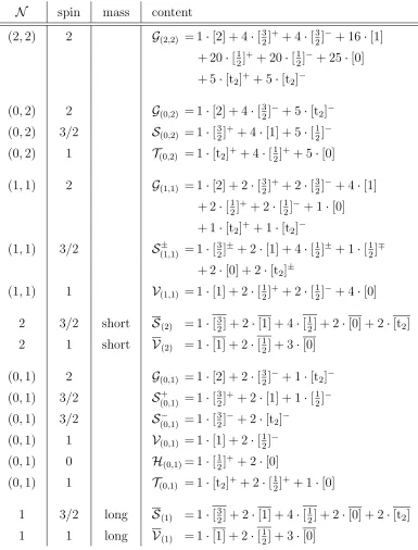
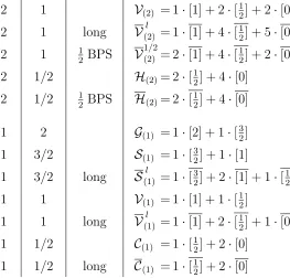
The perfect setting to provide further evidence for the conjecture is asymmetric Gepner models with more supersymmetry. They should correspond to supergravity theories that, constrained by the large amount of supersymmetry, only allow for definite supersymmetry breaking patterns. In the publication [3] we therefore classify all asymmetric Gepner models in four, six and eight dimensions with more than eight supercharges. Indeed we find all models either satisfy the constraints from gauged supergravity or can be explained by other mechanisms.
Having only an indirect geometric interpretation of non-geometric backgrounds there is still the question of what the intrinsic geometry of non-geometric backgrounds is. There are hints that the non-geometric nature manifests itself in the presence of the non-associative algebra
[xi, xj] = i 3~`
4
sR ijkp
k and [xi, pj] =i~δij.
wherels is the string length and Rµνσ is a constant antisymmetric tensor called theR-flux that is the fully T-dual flux to the knownH =dB flux. The algebra is non-associative and violates the Jacobi identity, both by a defect term∼Rijk. To quantize the algebra we will use deformation quantization algebras where a given algebra is realized by introducing a star product. For the above algebra the star product reads
f ? g=f ·g+12i~(∂if∂˜pig−∂˜pif ∂ig) + il4
s
6~R
ijkp
k∂if ∂jg+. . . ,
and indeed by inserting x and p we recover the above algebra. The appearance of a associative star product is intriguing since quantum mechanics usually forbids non-associativity by assumption and the conformal field theories of string theory are ordinary quantum theories. But so far in all calculations the contradiction could be resolved and the non-associative defects vanish by momentum conservation, the strong constraint of double field theory, or by only giving boundary terms without contribution to observables.
we follow the usual steps in constructing Einstein’s gravity and adjust every ingredient accordingly to the star product.
In a first step a star generalization to the diffeomorphism has to be found. To reconcile star products with a symmetry there are two approaches. The first introduces a star symmetry by changing the way the symmetry acts on fields. Since star symmetries do only exist for associative star products and the symmetry group U(N), we have to stick to the second approach, called twisted symmetries. In twisted symmetries, instead of changing the symmetry, the Leibniz rule is changed, or twisted, to guarantee covariance between the symmetry and the star product. Since twisted diffeomorphisms exist and appear naturally for non-associative star products, we will take this approach. We review the known procedure to define twisted tensors, twisted connections and a twisted Riemann curvature tensor. We fill existing gaps like the introduction of covariant derivatives of vectors or the introduction of the torsion tensor. But in doing so we find that the non-associative nature of the algebra leads to severe problems when introducing a metric. Let us mention two of them: Since the placing of the brackets between the three objects in a scalar product matters, there is no unambiguous generalization of a scalar product. Furthermore we can show that an inverse can only exist in very special cases. Ignoring these fundamental problems, we nevertheless try to find hints on how to reconcile the star gravity with the expectations of string theory. We find no obvious mechanism how to restore the usual diffeomorphism symmetry of string theory and associativity.
Conformal field theories of
Calabi-Yau compactifications
This chapter will review conformal field theories that describe superstring motion in a spacetime M10D =R3,1⊗Y3 where R3,1 is a flat Minkowski spacetime and Y3 is a
Calabi-Yau manifold defined as a hypersurface of a weighted projective space. This is one of the few string vacua where one knows both a supergravity description and the full classical string solution in terms of a conformal field theory. These conformal field theories were found by Doron Gepner and are accordingly called Gepner models. The aim of this section is to understand Gepner’s construction and especially how these highly abstract CFTs can be given a geometric interpretation in terms of a Calabi-Yau manifold. We will introduce the essential techniques such as the usage of simple currents, the computation of Hodge numbers or reading off the monomials from a CFT spectrum. All these techniques are employed later in the following main chapters and therefore the key to understand them.
The chapter starts with a short recap of Calabi-Yau compactifications from the super-gravity viewpoint while the rest of the chapter will be dedicated to conformal field theories. After introducing general features of the partition function we present certain conformal field theories that will be used as building blocks in Gepner’s construction. Afterwards we will turn to simple currents, a systematic method to construct modular invariant partition functions. In the fourth section we will reviewN = 2 superconformal field theories and why they necessarily appear in supersymmetric compactification of string theory. Subsequently we will introduce a class of N = 2 superconformal field theories, the Landau-Ginzburg models, that also turn out to be the minimal series of N = 2 superconformal field theo-ries. Then we will see how hypersurfaces in weighted projective spaces, thus Calabi-Yau manifolds, are actually described by Landau-Ginzburg orbifolds. After a short intermezzo about the computation of the Hodge data of these Calabi-Yau manifolds we will take all the building blocks and put them together into Gepner models.
2.1
IIB string theory on Calabi-Yau threefolds
When compactifying type IIB string theory on a Calabi-Yau threefold Y3 we get N = 2
target space supersymmetry in four dimensions. This chapter is meant as a reminder of known facts about the Kaluza-Klein compactification on a compact Calabi-Yau manifold and to introduce notation we need later.
To get an intuition about the Kaluza-Klein compactification let us take a massless 10D scalar φ and see what happens when splitting the spacetime as M10D = R3,1 ×Y3. In
particular the equations of motion will split
10Dφ=4Dφ+ ∆Y3φ = 0. (2.1.1) To get an effective four-dimensional description, φ is expanded in terms of eigenfunctions Yn of the internal Laplacian ∆Y3
φ(x, y) =X n
φn(x)Yn(y). (2.1.2)
The internal coordinates are calledyand the external onesx. When writing the eigenvalue equation as ∆Y3Yn =−m2nYn the equation of motion becomes
(4D −m2n)φn(x) = 0. (2.1.3) This reveals that φn is a scalar with mass mn in four dimensions. When repeating the analysis for p-forms one obtains a qualitatively similar result. In energy regions where E < mn we can truncate the spectrum to only the massless modes. To do so the internal part of any form has to be harmonic, thus eliminated by ∆Y3. Due to
∆Y3 =dd∗+d∗d , (2.1.4) where d∗ = ±? d?, a p-form ωp is harmonic if and only if ωp is closed dωp = d∗ωp = 0. Hodge’s theorem states that any p-form ωp has a unique decomposition
ωp =hp +dαp−1+d∗βp+1, (2.1.5)
where hp is a harmonic p-form. Therefore the harmonic forms are in the cohomology quotient
Hp(Y3) =
{dαp = 0}
{αp =dβp−1}
. (2.1.6)
the Betti numbers bp = dim(Hp(Y
3)). In the following we are using that any Calabi-Yau
manifold is a complex manifold and introduce holomorphic and antiholomorphic coor-dinates. Accordingly the cohomology is split as Hp,q(Y3) where p, q denotes the
holo-morphic/antiholomorphic dimension. The dimensions are denoted as Hodge numbers hp,q = dim(Hp,q(Y
3)).
We will now explicitly expand the 10D forms into the harmonic forms of the Calabi-Yau to obtain the massless 4D spectrum. The 4D indices will be Greek letters while the Calabi-Yau indices are named i, j,¯i,¯j and so on.
NS-NS Sector
There are two kinds of deformations of the metric that preserve the Ricci-flatness, the complex structure and the K¨ahler deformations. The complex structure deformations are controlled by the third cohomolgy group of the Calabi-Yau Y3 since the complex structure
is fixed by the choice of the holomorphic threeform Ω. In terms of a symplectic basis
{αΛ, βΛ} ∈H3(Y3) with Λ = 0, . . . , h2,1, the holomorphic threeform Ω is
Ω =XΛαΛ−FΛβΛ = αΛ, βΛ
·V2, (2.1.7)
where V2T = (XΛ,−FΛ). The periods XΛ span projective coordinates on the complex
structure moduli space. Fixing the projective freedom can be done by introducing za = Xa/X0wherea= 1, . . . , h1,2. Since the other coefficientsF
Λcan be computed as derivatives
of a prepotentialFΛ=∂F/∂XΛ, the complex structure is completely characterized by the
position on the manifold spanned by the za. Using the period matrix N (see e.g. the appendix of chapter 14 in [9]) one can build the matrix
M1 =
1 ReN
0 1
−ImN 0
0 −ImN−1 1
0 ReN 1
, (2.1.8) that we only state for later reference. For the even cohomology of the Calabi-Yau we introduce the basis
{ωA}={1, ωA and {σA}= √g
V dx
6
, σA , A= 0, . . . , h1,1 (2.1.9) whereV is the volume of the Calabi-Yau. {ωA} ∈H1,1(Y3) is a basis of the two-forms while
{σA} ∈H2,2(Y
3) is a basis of the four-forms. Therefore the index Aruns from 1, . . . , h1,1.
The second class of Ricci-flatness preserving deformations is called K¨ahler deformation. These deformations parametrize the size of the two-cycles and can therefore be collected into a two-form, the K¨ahler formJ. We can expand J and the internal part of the Kalb-Ramond field Bi¯j into the above basis
J =tAωA, B =bAωA. (2.1.10) Together they form the complexified K¨ahler form J =B+iJ appearing in
eB+iJ =eJ = ωA, σA
where V1 is
V1 =
1 JA 1
6κABCJ
AJBJC
1
2κABCJ
BJC
. (2.1.12)
κABC is the triple intersection number κABC = R
Y3ωA∧ωB ∧ωC. The complexified K¨ahler form J contributes complex scalars in 4D. Further NS-NS scalars are the dilaton φ and the Hodge dual ˜φ of the Kalb-Ramond field Bµν.
Using the period matrix of the K¨ahler sector we can built a similar matrix as (2.1.8) that we call M2.
Ramond-Ramond sector
In the following we will discuss the massless 4D fields from the R-R-sector. Let us start with the scalars. There is a single scalar from the C0 form and another scalar from the
Hodge dual of (C2)µν. The two-form C2 contributes further scalars from the components
(C2)i¯j. The self-dual four-form gives scalars by Hodge dualizing (C4SD)µνi¯j into scalars. Having the dualization in mind one can summarize all the scalars from the R-R-forms as
C
scal. = ˜ξ0+ξ Aω
A+ ˜ξAσA+ξ0ω0 = ωA, σA
·Ξ. (2.1.13) The democratic formulation C = C0 +C2 +C4 +C6 is used here and the (2h1,1 +
2)-dimensional vector Ξ contains the R-R axions ΞT = (ξA,ξ˜ A).
The R-R-sector contributes vectors by putting the self-dual four-form C4SD on three-cycles (CSD
4 )µijk, (C4SD)µijk¯, (C4SD)µi¯j¯k and (C4SD)µ¯i¯jk¯. Expansion into the above basis yields C4 =AΛαΛ+ ˜AΛβΛ, (2.1.14)
where (A,A) are the four-dimensional vector fields. Only half of them are actually inde-˜ pendent due to the self-duality of the four-form. As such there are only h1,1 + 1 vectors
from the R-R-sector.
Summary
To summarize, the bosonic massless spectrum of type IIB on a Calabi-Yau and their 10D origin is P P P P P P P PP 4D 10D
C0 C2 C4SD φ B2 g
g - - - 1
2-Form/Scalar - 1 h1,1 - 1
-Vector - - h1,2+ 1 - -
The N = 2 massless multiplets have the following particle content
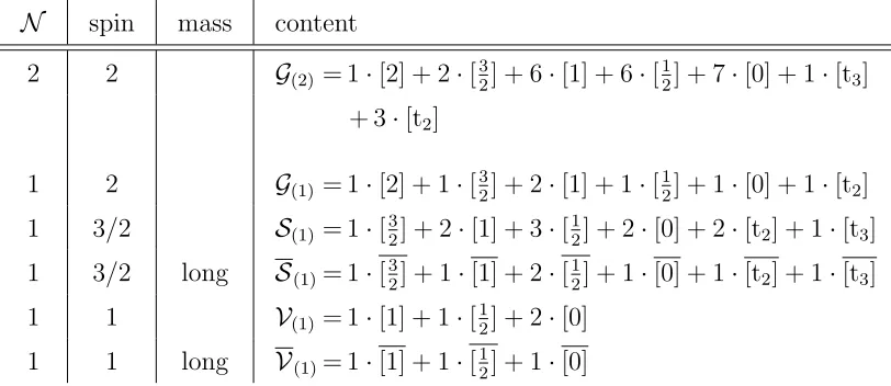
masslessN = 2 gravity G(2) = 1·[2] + 2·[32] + 1·[1] = (2)b+ (4)f+ (2)b,
masslessN = 2 vector V(2) = 1·[1] + 2·[12] + 2·[0] = (2)b+ (4)f+ (2)b,
masslessN = 2 hyper H(2) = 2·[21] + 4·[0] = (4)f + (4)b.
(2.1.15)
The first equality states the number of particles of each spin, while the second equal-ity counts the fermionic and bosonic degrees of freedom of each spin. The massless IIB spectrum in 4D falls into the N = 2 multiplets as follows
massless N = 2 gravity G(2) ⊃ gµν, A0
, massless N = 2 vector V(2) ⊃ Aa, za
,
massless N = 2 hyper H(2) ⊃ J
A, ξA, ξ˜ A
,
Huniv.
(2) ⊃ φ , φ , ξ˜ 0, ξ˜0
.
(2.1.16)
The 4D IIB spectrum has NV =h1,2 vector multiplets andNH =h1,1+ 1 hypermultiplets next to the obligatory supergravity multiplet.
The scalars of the vector multipletsza are the coordinates on a special K¨ahler manifold. The 4(h1,1+ 1) scalars of the hypermultiplets are the coordinates of a special quaternionic
K¨ahler manifold that has a fibration structure in which the base is spanned by the complex K¨ahler moduli JA that form a special K¨ahler manifold.
2.2
Conformal field theory
This section starts with a small review about partition functions and related topics like characters or modular invariance. Then we will shortly recap Kac-Moody algebras and present selected conformal field theories that we need later as building blocks for Gepner models.
2.2.1
Partition functions and related topics
The one-loop diagram of a closed string theory is a worldsheet with one hole, a torus. Computing quantum corrections is therefore done by looking at conformal field theories on a torus. Similar to quantum field theory also in string theory every particle can run in the loop. The probability for a particle to run in a loop is given by a Boltzmann factor. This notion gives rise to the partition function
Z(τ,τ¯) = TrH e−2πHIm(τ) e+2πPReτ
= TrH
qL0−24c q¯L0¯ − ¯
c
24
whole Hilbert-space of the conformal field theory reflecting that all particles can run in a loop. L0 are the zero modes of the Virasoro-algebra
[Lm, Ln] = (m−n)Lm+n+ c 12(m
3−m)δ
m+n,0, (2.2.2)
that generate conformal transformations. The zero modes L0 ±L¯0 generate translations
in time and space and the eigenvalue ofL0 is the conformal dimensionh of the state. The
energy isH =L0+ ¯L0−c24+¯c where the central charge termc,¯cis a normal ordering constant.
In contrast to the quantum field theory case also a term with the momentum−iP =L0−L¯0
appears in the exponent of the partition function since the string worldsheet is spread over both time and space. When expanding the partition function according to the energy, one can read off the number of states at each energy level E by looking at the coefficient of the exponential e−2πEIm(τ). In particular, massless states must have h= 24c and appear as constant piece in the expansion. Usually one expands only sectors of the partition function, since bosons and fermions contribute with a different sign to the partition function such that in target space supersymmetric theories Z = 0.
Modular invariance
The complex parameterτ with Im(τ)>0 appearing inq =e2πiτ parametrizes the complex structure of the torus C
Z+τZ. To be well defined in string theory the partition function
(2.2.1) has to be invariant under the global diffeomorphism of the torus that are the modular transformations
SL(2,Z)/Z2 : τ →
aτ +b
cτ +d, where
a b c d
∈SL(2,Z)/Z2. (2.2.3)
The generators of this group are the modular transformations
S :τ → −1
τ and T :τ →1 +τ . (2.2.4) The torus partition function and therefore the possibilities to combine left- and right-movers is highly constrained by modular invariance. Finding and classifying non-trivial partition functions is a hard task and has only been achieved in special cases.
Highest weights and conformal families
The spectrum of a conformal field theory can be characterized by stating the highest weights
|φii of the theory. These states are annihilated by every single annihilation operators Ln|φii= 0, for n >0, L0|hi=hi|φii. (2.2.5)
The vacuum is always a highest weight and usually denoted byi= 0. All other states can be constructed from the highest weight by applying the creation operator of the symmetry algebra, e.g.
|φii, L−1|φii, L−2|φii, L−1L−1|φii, . . . . (2.2.6) These states form the conformal family [φi]. By the operator-state correspondence the descendants of φi correspond to the field φi, its derivatives and normal ordered products of φi together with the energy-momentum tensor.
Characters, the modular S-matrix and the Verlinde formula
Since the highest weights define separate sectors of the theory one can split the partition function into the contribution of the different highest weights. The contribution of a highest weight defines the character
χi = trHi q
L0−c
24 . (2.2.7)
The trace runs only over the left-moving Hilbert space Hi that is associated to the high-est weight with index i, therefore the whole conformal family [φi]. Under a modular T-transformation the character is multiplied with a phasee2πi(hi−24c) while under a
modu-lar S-transformation the characters of the different highest weights mix. This mixing can be parametrized by the modular S-matrix in the following form
χi −τ1
=Sijχj(τ). (2.2.8) The modularS-matrix is usually symmetric, unitary and squares to the charge conjugation matrix.
When computing the OPE of a field in [φi] with a field in [φj] one finds that only the fields of some conformal families appear. This gives rise to the fusion algebra
[φi]×[φj] =Nijk [φk], (2.2.9) that schematically captures which conformal families appear in each others OPEs. One of the deepest results of conformal field theory is the Verlinde formula. It states that the fusion coefficients Nijk can be expressed in terms of the modular S-matrix as
Nijk =X m
SimSjmSmk∗ S0m
where the sum runs over all highest weights and 0 labels the vacuum highest weight. This formula connects tree-level (sphere) and one-loop (torus) amplitudes in an intriguing manner.
In terms of the characters (2.2.7) the partition function (2.2.1) can be written as
Z(τ, τ) =χi(τ)Mijχj(¯τ). (2.2.11) The matrixM collects how the highest weights from the left and the right are combined to target space fields. To guarantee modular invariance we infer [M, S]= 0. Finding a non-! trivialM 6= 1 with [M, S]=0 is a hard task. Invariance under the modularT-transformation is guaranteed if
hi−hj ∈Z (2.2.12)
together with c=c.
2.2.2
Kac-Moody algebra
Most theories we will review in the following have a Kac-Moody symmetry. These algebras capture, that the algebra of the currents Ja generating the symmetry may have a central extension from normal ordering. The modes ja
n of the Kac-Moody algebra ˆgk at level k obey
[jma, jnb] =ifabc jmc+n+k m δm+n,0 δab, (2.2.13)
where thefabc are the structure constants of the underlying Lie algebrag. One can define an energy momentum tensor according to Sugawara’s construction
T(z) = 1 2(k+Cg)
N(JaJa)(z), (2.2.14)
where N(. . .) denotes the normal ordering and Cg is the dual coxeter number of g. One can expand T(z) into
T(z) =X n
z−n−2Ln. (2.2.15) where the modes Ln are
Ln = 1 2(k+Cg)
X l≤−1
jlajna−l+X l>−1
jn−ljl !
, (2.2.16)
since the normal ordering places annhihilation operators to the right. Using the Kac-Moody algebra of the currents one can show that the modes Ln obey the Virasoro-algebra (2.2.2). Furthermore the commutator
reveals that the currents have conformal dimension one. For the central charge of the CFT one finds
c= k dimg k+Cg
, (2.2.18)
where dimg is the dimension of the Lie algebra g.
2.2.3
so
b
(
N
)
1and the bosonic string map
When looking at string theory on a space with 10−D compact internal directions, the remaining external directions have a SO(D−1,1) Lorentz symmetry. The usage of light-cone gauge effectively eliminates two dimensions and the massless states transform under the little groupSO(D−2). To describe the external directions from the worldsheet point of view we need N =D−2 free bosons and their superpartners,N =D−2 free fermions transforming in the vector representation of SO(N). The CFT for the N fermions is the
b
so(N)1 CFT that must have central charge c=N/2 due to the field content. This central
charge is consistent with (2.2.18) when inserting Cg =N −2 and dimg= 12N(N −1). Having fermions we have two separate sectors, the NS and the R sector. Both, the R and the NS sector can further be split into states with even and odd fermion number. The resulting four sectors correspond to the four highest weights of the theory. The first NS highest weight is the true vacuum whose sector we name O. The second NS highest weight is Ψi
−1/2|0i. Due to its transformation behavior this sector is called vector V. In
the R sector we have zero modes satisfying the Clifford algebra such that the groundstate is degenerate and transforms as a spinor. The fermion number translates into the chirality that distinguishes the two subsectors of the Ramond sector. We name these two sectors the spinor S and antispinorC.
In the following we only have D = 4,6,8 non-compact directions thus even N = 2n. Let us present a collection of the relevant properties of sob(2n)1.
character h q mod 2 degeneracy O = 12 θ3η
n +θ4η
n
0 0 0
V = 12 θ3η n
−θ4 η
n
1
2 1 2n
S = 12 θ2η n
+θ1η n
n
8
n
2 2
n−1
C = 12 θ2η n
−θ1 η
n
n
8
n
2 −1 2
n−1.
(2.2.19)
functions. The modularS-matrix of the sob(2n)1 theory is
Ssob(2n)1 = 1
2
1 1 1 1
1 1 −1 −1 1 −1 i−n −i−n 1 −1 −i−n i−n
. (2.2.20)
Using the Verlinde formula (2.2.10) the fusion rules are
n odd o v s c n even o v s c
o o v s c o o v s c
v v o c s v v o c s
s s c v o s s c o v
c c s o v c c s v o.
(2.2.21)
The bosonic string map
b
so(2n)1 describes 2n fermions that we can bosonize into n free bosons on a circle of radius
R = √2α0. This suggests that we can take a partition function of a fermionic string and
turn it into a bosonic string partition function.
There are two major problems. The first one is the mismatch in the central charge. A conformal field theory in bosonic string theory hasc= 24 while a conformal field theory for a fermionic string has c= 12. We have to find an additional ingredient that accounts for the ∆c= 12. The second problem is that the mapping has to preserve modular invariance. When looking at the modularS-matrix of sob(2n)1 in (2.2.20) we see that it is invariant
under n → n + 4. This suggests that we map the characters of sob(D −2)1 onto the
characters ofsob(D+ 22)1. In this way both the central charge is taken care of and modular
invariance is preserved. The only obstacle is that the conformal dimension1 of the R states
shifts by 3/2 under the mappingsob(D−2)1 ↔sob(D+ 22)1 while the NS states keep their conformal dimension. The level matching condition of modular T-invariance hL−hR ∈Z is therefore broken for R⊗NS and NS⊗R states. This can be cured by mapping the charactersO andV onto each other, since their conformal dimension differs by 1/2. When interchanging O andV the S-matrix is only invariant if we simultaneously interchange the characters (S, C) with either (−C,−S) or (−S,−C). Notice that both choices (−C,−S) or (−S,−C) are connected by charge conjugation. Since a charge conjugation interchanges IIA and IIB, starting with a bosonic partition function we can arrive both at a IIA and a IIB partition function. For IIB we take the same convention for both sides while for IIA we have to use different choices for the left- and right-movers. Since a charge conjugation is easy to apply in the CFTs we are looking at, we can stick to one choice and apply charge
conjugation afterwards. In the following we will take the choice (S, C) ↔ (−C,−S). A practical reason for this is that we assign a number s0 = (0,2,−1,1) to each of the four
characters (0, V, S, C).The mapping then amounts to s0 →s0+ 2 mod 4 which is easy to
realize in a computer program.
To summarize, we have a map calledbosonic string map which maps a fermionic string partition function onto a bosonic string partition function via
φbsm(O, V, S, C)∈sob(D−2)1 →(V, O,−C,−S)⊗1∈sob(D+ 22)1. (2.2.22) where O, V, S, C denote the characters (2.2.19). When applying the bosonic string map onto only say the right-movers we get a heterotic string partition function that descents from the SO(32) heterotic string.
By the same arguments as above, a similarly looking map maps the characters of
b
so(D−2)1 ↔sob(D+ 6)1 onto each other without spoiling modular invariance. But then we have to find another explanation where the remaining 8 units of central charge are coming from. The solution lies in the other heterotic string theory, the E8×E8 heterotic
string. Noticing thatSO(D+ 6) is a subgroup ofE8, the missingc= 8 can be attributed to
the 8 free bosons on the root lattice of the other E8 factor in theE8×E8 heterotic string.
This is consistent since (ˆe8)1 has only a singlet representation with conformal dimension 0.
Therefore the additional (ˆe8)1 factor does not change the way the states are mapped onto
each other but can cure the mismatch in the central charges. The second bosonic string map is
φbsm(O, V, S, C)∈sob(D−2)1 →(V, O,−C,−S)⊗1∈sob(D+ 6)1⊗(ˆe8)1. (2.2.23) There are therefore two consistent bosonic string maps. The choice of bosonic string map is only relevant when looking at massive states or when constructing heterotic partition functions. Since we only consider the massless type IIB spectrum we in principle do not have to specify which one we take. In our computer programs we decided to work with the
b
so(D−2)1 →sob(D+ 6)1⊗(ˆe8)1 bosonic string map.
Target space interpretation
Thesob(D−2)1 theory is the CFT of the uncompactified directions. Being the little group,
the transformation behavior under this symmetry tells us about the particle interpretation from theD-dimensional viewpoint. In closed string theory every state combines a left- and right-moving sob(D−2)1 state. In the following we will state which target space particle
appears for every combination of thesob(D−2)1 highest weights. We will restrict ourselves
to massless modes. Universal in all dimensions is
V ⊗V → gµν+Bµν +D , V ⊗O → Aµ,
O⊗O → φ ,
where g is the metric, B is the Kalb-Ramond field, D is the dilaton. φ is a real scalar while Aµ is a vector. Using (2.2.19) one can check that the number of degrees of freedom is correct. All other tensor products involve the spinorial degrees of freedom and their decomposition depends on the number of non-compact directions. The target space fields can be recovered either by group theory or more easily by counting the degrees of freedom and following the fusion rules (2.2.21).
In case of four non-compact dimensions D= 4 we find D= 4 : S⊗C → φ ,
S⊗S, C ⊗C → 1 2V ,
(2.2.25)
where 1
2V denotes one of the two degrees of freedom of a massless vector in four dimensions.
In six non-compact dimensions D= 6 one finds
D= 6 : S⊗C → Aµ
S⊗S, C ⊗C → φ+Tµν(A)SD, (2.2.26) where Tµν(A)SD denotes a self-dual or anti-self-dual two-form with three degrees of freedom characteristic for chiral 6D theories. An important fact is that in chiral theories the ten-sors that are part of tensor multiplets must either all be self-dual or all be anti-self-dual. Accordingly the B field from (2.2.24) has to be split into a self-dual and an anti-self-dual part. The part that has the same chirality as the remaining tensors forms another tensor multiplet, while the other part will be part of the supergravity multiplet. Finally in 8D we have
D= 8 : S⊗C → φ+Cµν, S⊗S, C ⊗C → Aµ+ 12Cµνρ.
(2.2.27)
2.2.4
A free boson on a circle of radius
R
=
√
2
k
The partition function of a free boson on a circle of radius R is
Zcirc.(τ, τ) =
1
|η(τ)|2
X m,n∈Z
q12(
m R+
Rn
2 ) 2
q12(
m R− Rn 2 ) 2 . (2.2.28)
m is the quantized momentum along the circle, n is the winding number, q = e2πiτ and η(τ) is the Dedekind η function. For the special values R = √2k this theory is called b
u(1)k.2 As it turns out, for these special values of the radius the partition function can be written in terms of characters χ(mk)
Zbu(1)k(τ, τ) =
k X m=−k+1
χ(mk)
2
with χ(mk) = 1
η(τ) Θm,k(q) (2.2.29)
2Speaking of a level does not make sense for abelian algebras since the level can be chosen arbitrarily
labeled by an integer charge
m =−k+ 1, . . . , k . (2.2.30) The capital Θ functions are
Θm,k(τ) = X n∈Z+2mk
qk n2 .
(2.2.31)
The highest weight of each character has conformal dimension
h(mk)= m
2
4k , (2.2.32)
which can be seen by expandingη(τ)≈q−241 +. . . and comparing this with the definition of a character (2.2.7) due to the central charge being c = 1. The modular S-matrix for these characters is found to be
Sm,m0 =
1
√
2k exp
−πimm
0
k
. (2.2.33)
2.2.5
The
su
b
(2)
kKac-Moody algebra
Another important building block we need later is thesub(2)k theory. The structure coeffi-cents in (2.2.13) are the ones of su(2), fabc =√2abc where is the purely antisymmetric tensor in three dimensions, therefore dimg = 3 and the dual Coxeter number is Cg = 2. The central charge is according to (2.2.18)
c
b su(2)k =
3k
k+ 2. (2.2.34)
Let us look at the highest weight states of this CFT. The Cartan subalgebra consists of L0 and j03. A highest weight has therefore two quantum numbers |h, qi, the conformal
dimension h and the charge defined by ˆj3
0|h, qi = q|h, qi. For convenience we defined
ˆ j0i = √1
2j
i
0. The ˆj0i form an su(2) subalgebra whose representation theory is well known
from quantum mechanics. Unitary highest weights representations with a certain conformal dimension have a spin 2l labeled by a positive integer l ∈N0. The spin in the z direction
is labeled by another number α∈0, . . . , l stating how often we went down the ladder from the highest state. With every step in the ladder the charges decreases by two such that the charge of a state is q=l−2α. For the conformal dimension one finds
h= l(l+ 2)
4(k+ 2). (2.2.35)
The values ofk andlare further constrained since there are moresu(2) subalgebras hidden in the Kac-Moody algebra. For them to have integer eigenvalues and to guarantee non-negative norm states one has to demand
Having the highest weights let us state their characters. It is useful to define generalized characters that sort each state not only with respect to their conformal dimension but also according to their charge
χ(lk)(τ, z) = trHl
qL0−24c e−2πizˆj 3 0
. (2.2.37)
The result can be computed using the Weyl-Kac character formula [10]
χ(lk)(τ, z) = Θl+1,k+2(τ, z)−Θ−l−1,k+2(τ, z) Θ1,2(τ, z)−Θ−1,2(τ, z)
, (2.2.38)
where the generalized Θ functions are defined by
Θl,k(τ, z) = X
n∈Z+2lk
qk n2 e−2πinkz.
(2.2.39)
In the definition (2.2.37) one can infer that for z = 0 the generalized Θ functions become the usual Θ functions (2.2.31) and one should recover the usual characters appearing in the partition function. But this is not possible in (2.2.38) which would render the fraction ill defined. Therefore, one rather has to take the limit z → 0. The form (2.2.37) is in particular useful to determine the modular S-matrix for which one finds
Sll(k0) =
r 2 k+ 2sin
π
k+ 2 (l+ 1)(l
0
+ 1)
. (2.2.40)
Using the Verlinde formula the fusion rules are
Nl1l2l3 = 1 for|l1−l2| ≤l3 ≤min(l1+l2,2k−l1 −l2) andl1+l2+l3 even
Nl1l2l3 = 0 else. (2.2.41)
Level Z Name
k =n Pnl=0|χl|2 An+1, n≥1
k = 4n Pnl=0−1|χ2l+χk−2l|2+ 2|χk/2|2 D2n+2, n≥1
k = 4n+ 2 Pk/l=02|χ2l|2+P2n
−2
l=0 χ2l+1χk−2l−1 D2n+1, n≥2
k = 10 |χ0+χ6|2+|χ3+χ7|2+|χ4+χ10|2 E6
k = 16 P
l=0,4,6|χl+χ16−l| 2+ (χ
2+χ14)χ8+χ8(χ2+χ14) +|χ8|2 E7
k = 28 |P
l=0,10,18,28χl|2+| P
l=6,12,16,22χl|2 E8
.
(2.2.42)
Let us establish a relationship between thesub(2)1 and thebu(1)ktheories from section 2.2.4. Taking a free boson φ on a circle of radius R = √1
2, the vertex operators V± =e
±i√2X are currents since they have conformal dimension one. Together with the usual currentj =i ∂φ they form ansub(2)1 Kac-Moody algebra. On the other hand this theory can be T-dualized
to radius R0 =√2 which is the bu(1)1 theory. The equivalence of thesub(2)1 and bu(1)1 can be checked by comparing the spectrum and indeed, both have exactly two highest weight states of conformal dimension 0 and 14.
Computing the partition function of this theory would be hard in thesub(2)1 theory due to the complicated Weyl-Kac character formula (2.2.37). But for the dual bu(1)1 the more
tractable formula (2.2.29) tells us
Z(τ, τ) = 1
|η(τ)|2 |Θ0,1| 2+|Θ
1,1|2
. (2.2.43)
As it turns out we can in general express the character (2.2.37) of the sub(2)k theory in terms of the Θ functions. Indeed, there is an expansion [11]
χ(lk)(τ) = X
m=−k+1,...,kandl+meven
Cl,m(k)(τ) Θm,k(τ), (2.2.44) where theCl,m(k)(τ) are called string functions. In this expansion the string functionsCl,m(k)(τ) encode how the bu(1)k theory is embedded into the sub(2)k theory. In the above example (2.2.43) they were constant but for higherk they are not. They are explicitly computed in [11].
2.3
Simple currents
Schellekens and Yankielowicz in [12]. Simple currents Ja are defined by their particular simple fusion rules. The fusion product of a simple current with any other primary must result in exactly one primary
[Ja]×[φi] = [φJ(i)]. (2.3.1)
Actually, most theories have simple currents. For instance looking back at the fusion rules of the sob(2n)1 theory in (2.2.21) we see that any highest weight of this theory is in fact a
simple current. By associativity, the product of two simple currents is a simple current as well. Assuming a finite amount of primaries in our theory there must exist a number Na for whichJNa
a = 1. We will denote the number Na as the length of the simple current. The simple currents{Ja, Ja2, . . . , J
Na
a }form a finite abelian subgroup ZNa of the fusion algebra
and there exists a fusion inverse of every simple current (Jn a)
−1 = JNa−n
a . Consequently, every simple current groups the conformal primaries into orbits of length Ni
a
{φi, Ja×φi, Ja2×φi, . . . , JNai−1
a ×φi}. (2.3.2) Since JNa
a = 1, the length of the i-th orbit Nai must be a divisor of Na. Translating the fusion rule (2.3.1) of a simple current into an OPE results in
Ja(z)φi(w)∝
φJ(i)(w)
(z−w)Q(ia) + desc. , (2.3.3) where Q(ia) is called monodromy charge. The name is chosen since Q(ia) mod 1 denotes the monodromy e−2πiQ(ia) when circling the simple current around the primary (z−w) →
e2πi(z−w). By applying J
a(z) onto the last formula untilJaNa = 1 appears shows Q(ia) = t
i a
Na
mod 1, tia∈Z, (2.3.4)
since the monodromy of the identity is Q(0a) = 0 mod 1. Probably the easiest way to compute the monodromy charge uses the formula
Q(ia) =h(φi) +h(Ja)−h(Ja×φi) mod 1 . (2.3.5) Repeating the same steps that lead to (2.3.4) for the OPE of simple currents one finds
Ja(z)Ja(w)∝ J2
a(w) (z−w)Nraa
+ desc. . (2.3.6)
For simple currents we give the parameter ti
a the special letter ra and its own name, the
monodromy parameter. To compute the monodromy parameterra we deduce from (2.3.6) 2hJa =hJa2 +
ra
Na
and by iteration
hJn a =ra
n(n−1) 2Na
+nhJa mod 1. (2.3.8)
UsinghJNa
a =h1 = 0 mod 1 results in
hJa =ra
Na−1 2Na
mod 1. (2.3.9)
This relation was used in our computer programs to compute the monodromy parameter ra for a simple current. Notice that ra must be defined modulo Na for odd Na while for even Na we must have ra modulo 2Na to cover all cases. When ra is known, one can also deduce a relation for the monodromy charge of the field Janφi that appears in the OPE Ja(z1). . . Ja(zn)φi(w). Recall that the monodromy charge denotes the mon-odromy when going around the primary of interest with the simple current, therefore for Ja(z1). . . Ja(zn)φi(w) a monodromy encircling all zi and w. By deforming the contour the full monodromy must be the sum of each of the individual monodromies. Using this we compute
Q(a)(Janφi) =Q(a)(φi) +n Q(a)(Ja) =
ti+ran
Na
mod 1. (2.3.10) As a corollary we find that if the simple current has integral conformal dimension, thus ra = 0, every primary in an orbit has the same monodromy charge. Such simple currents are called orbit simple currents.
With all this machinery established let us come to the key observation by looking at a generic OPE between two primaries
φi(z)φj(w) = X
k
ckij(z−w)hk−hi−hjφ
k(w) + desc. . (2.3.11)
Taking a monodromy with respect to a simple current Ja on both sides one finds
Q(a)(φi) +Q(a)(φj) = Q(a)(φk). (2.3.12) Therefore the monodromy charge is actually a conserved quantity. When modding out this symmetry by an orbifold-like procedure with twist e2πi(QL(a)+Q(Ra)), we get a new partition
function. In the seminal paper [12] the authors use this twist very explicitly. Here we directly state the matrix M appearing in the partition function (2.2.11)
Z(τ, τ) = χi(τ)Mijχj(τ) (2.3.13) that for a simple current Ja reads
(M(Ja))kl =
Na
X p=1
where ˆQ(a)(φ
i) is half the monodromy charge
ˆ
Q(a)(Jpφi) = ti+rp 2Na
mod 1, (2.3.15)
and δ(1) is a delta function modulo one. The delta function can also be written as δ
Q(φk) + rp 2Na
, (2.3.16)
where pdenotes the power of the simple currents acting on φk. An important obstruction is that the proof of modular invariance of the partition function relies on ra being even. Sincera is defined moduloNa or 2Na one can chooserato be even except whenNais even and ra is odd.
Roughly speaking, the matrix Main (2.3.14) induces a partition function that connects a left-moving primary to its whole right-moving orbit if the monodromy charges add up to an integer. For instance, for orbit simple currents with hJa = 0 where ra= 0 the partition
function is of the form
Z = X
Orbits
|χφ+χJ φ+· · ·+χJNa−1φ|2. (2.3.17) The sum is understood to run over all orbits in which the monodromy charge is an integer. The partition function of orbit simple currents contains only perfect squares such that it is left-right symmetric.
Modular invariance is not spoiled when using more than one simple current in a partition function
Z ∼ ~χT(τ)M(J1)M(J2). . . ~χ(τ), (2.3.18)
where we neglected a normalization constant to have a unique vacuum. In general the matrices of different simple currents do not commute making the order of the matrices very important. But there is a criterion to guarantee commutativity. The matricesM(J1)
and M(J2) commute if and only if the simple currentsJ1 and J2 are relatively local. This
property can be translated into a vanishing relative monodromy chargeQ1(J2) =Q2(J1) =
0.
Examples
Looking back at the classification of modular invariants of sub(2)k (2.2.42) one recognizes in (2.3.17) the form of theD2n+2 invariant. In the following we will recover theDpartition
function of sub(2)k with even k using the simple current technique. In a first step let us classify the simple currents ofsub(2)k. Playing around with the fusion coefficients ofsub(2)k, (2.2.41), one sees that the inequality
becomes l3 = k−l2 for l1 = k since l ≤ k. For l1, l2 6= k the inequality is satisfied for
more than one value ofl3. Therefore, there is one non-trivial simple currentJ = (k) in the
b
su(2)k theory besides the trivial one with l = 0 being the identity. The simple current J has length N = 2 and using (2.2.35) the conformal dimension is hJ = k4.
Let us start with k = 4n since then hJ = 1 = 0 mod 1 and thereforer= 0. The orbits are {φl, φk−l} and the monodromy charge is
Q(l) = l
2, (2.3.20)
thus Q = 0 mod 1 for even l and Q = 12 mod 1 for odd l. Due to (2.3.16) we may only have integer monodromy charge and every primary in an orbit is connected to any other primary in that orbit. The partition function is therefore
Z = n−1
X l=0
|χ2l+χk−2l|2+ 2|χk/2|2. (2.3.21)
Notice that the k2 orbit is {χk/2, χk/2} since the simple current acts as identity on the
primary with l = k2. Summing over the fields in the k2 orbit produces the same character χk/2 twice. To capture the factor of two, the χk/2 character is excluded from the sum. We
found the partition function of the D2n+2 series (2.2.42).
Next we look atk= 4n−2 where the conformal dimension of the simple currentJ = (k) is hJ =n− 12 = 12 mod 1. Using (2.3.9) the monodromy parameter is now r= 2 while the monodromy charge is still Q(l) = 2l. Recall (2.3.16)
δ
Q(φk) + rp 2Na
, (2.3.22)
where p denotes the amount of simple currents acting on the primary, thus p = 0,1. For even l whereQl = 0 mod 1 the delta function vanishes unlessp= 0. In words, a field with even l can only be coupled to itself and not to the other field in the orbit for whichp= 1. In contrast for oddl whereQl = 1/2 we needp= 1. Therefore an odd field can be coupled only to its partner in the orbit. The partition function is
Z = k/2
X l=0
|χ2l|2+
2n−2
X l=0
χ2l+1χk−2l−1, (2.3.23)
This is the D2n+1 invariant (2.2.42).
Let us see what happens for odd k. There hJ = 1+24n giving an odd r= 1 + 2n. Since
2.4
N
= 2
superconformal field theories
This section will review the salient features ofN = 2 superconformal field theories (SCFTs) [13, 14, 15]. Since this is textbook standard ([8, 9]) we will be brief and stick to those features relevant later.
Algebra
The conformal enhancement of the supergravity multiplet consists of the energy momentum tensorT(z) with its modesLm, two fermionic supercurrentsG±(z) with their modesG±m±a, where the real paramater a is a ∈ Z for the R sector while a ∈ Z+ 12 for the NS sector, and a currentJ(z) with modesjm. The modes satisfy the N = 2 superconformal algebra
[Lm, Ln] = (m−n)Lm+n+ c 12(m
3 −m)δ
m+n,0,
[Lm, jn] =−n jm+n, [Lm, G±n±a] =
m
2 −n∓a
G±m+n±a, [jm, jn] =
c
3 m δm+n,0, [jm, G±n±a] =±G
±
m+n±a,
{G+n+a, G−m−a}= 2Lm+n+ (m−n+ 2a)jm+n+ c 3
(m+a)2− 1
4
δm+n,0,
{G±, G±}= 0.
(2.4.1)
We infer that the quasi-primary T(z) has conformal dimension 2, the primaries G±(z) have conformal dimension 3/2 and the primary J(z) has conformal dimension 1. The current J(z) satisfies abu(1) Kac-Moody algebra which we recognize as R-symmetry, since the supercurrents G± have charge ±1. In the following, states |h, qi are labeled by their conformal dimensionhand theiru(1) chargeqthat are the eigenvalues of|h, qiwith respect to the cartan subalgebra L0 andj0. The definition of highest weight states (2.2.5) must be
adjusted to the enlarged symmetry algebra as follows:
G±n|h, qi= 0, forn >0, (2.4.2) from which similar statements for Ln and jn follow by use of the algebra (2.4.1). Using unitarity, 0≤ |G±0|h, qi|2, the bound
hR≥ c
24 (2.4.3)
can be derived for states in the Ramond sector. We recognize states saturating this bound as the Ramond groundstates.
In a similar fashion we can derive from 0 ≤ |G±−1/2|h, qi|2 the bound
for states in the NS sector. States saturate this bound if and only if they are annihilated by the supercurrent G±−1/2
G±−1/2 |h=±q/2i= 0. (2.4.5) Clearly the vacuum satisfies this equation. This equation and the bound 2h≥ |q| suggest that we found the conformal analogue of short multiplets, the BPS states. We will call states chiral and antichiral depending on whether they are annihilated by G+−1/2 orG−−1/2. Using 0≤ |G±−3/2|h, qi|2 one finds another bound for NS chiral primaries
6h≤c . (2.4.6)
The (anti)chiral fields close under fusion, and their OPE is non-singular as can be seen by dimensional analysis. As such the (anti)chiral fields define a multiplicative ring, called chiral ring or antichiral ring. When left- and right-movers are combined there are in total four rings that we call the (a,a), (c,a), (a,c) and the (c,c) ring.
For any state in the NS sector there is a unique orthogonal decomposition
|φi=|φ0i+G+−1/2|φ1i+G
−
−1/2|φ2i, (2.4.7)
where|φ0iis a chiral primary while |φ1i and|φ2iare not. This relation can be interpreted
as the worldsheet analogue of the Hodge decomposition of forms (2.1.5), when writing the Hodge decomposition in complex coordinates. The G+−1/2 and G−−1/2 are the analogues of the holomorphic derivatives∂, ∂∗ from the worldsheet point of view. For the right-moving counterparts we identify (oppositely)G−−1/2andG+−1/2with the antiholomorphic derivatives ∂, ∂∗. The anticommutator {G+−1/2, G−1/2} is then related to the internal Laplacian ∆∂ = ∆∂ = ∆ (2.1.4). Most importantly the chiral fields are on equal footing as harmonic forms and are therefore directly related to the topology, the non-trivially closed cycles.
In case of a Calabi-Yau threefold Y3 we find the following relation: The K¨ahler moduli,
being elements of H1,1(Y3), correspond to the (a,c) and (c,a) primaries while the
com-plex structure moduli, being elements of H1,2(Y
3), correspond to the (c,c) and the (a,a)
primaries.
The chiral ring, spectral flow and spacetime supersymmetry
In anyN = 2 SCFT there exists an automorphism of the algebra induced by the generators Uη called spectral flow operator [16, 17] where η ∈ R is a real parameter. Uη acts on an operator asLη
m =UηLmUη−1and on states as|hη, qηi=Uη|h, qi. The transformed operators are
Lηm =Lm+η jm+ c 6η
2
δm,0,
Gηm±±a =G
±
m±(a+η),
jmη =jm+ c
3η δm,0,