HIGHLIGHTED ARTICLE
GENETICS | INVESTIGATION
Bayesian Nonparametric Inference of Population
Size Changes from Sequential Genealogies
Julia A. Palacios,*,†,‡,1John Wakeley,* and Sohini Ramachandran†,‡,1
*Department of Organismic and Evolutionary Biology, Harvard University, Cambridge, Massachusetts 02138, and†Department of Ecology and Evolutionary Biology and‡Center for Computational Molecular Biology, Brown University, Providence, Rhode Island 02912
ABSTRACTSophisticated inferential tools coupled with the coalescent model have recently emerged for estimating past population sizes from genomic data. Recent methods that model recombination require small sample sizes, make constraining assumptions about population size changes, and do not report measures of uncertainty for estimates. Here, we develop a Gaussian process-based Bayesian nonparametric method coupled with a sequentially Markov coalescent model that allows accurate inference of population sizes over time from a set of genealogies. In contrast to current methods, our approach considers a broad class of recombination events, including those that do not change local genealogies. We show that our method outperforms recent likelihood-based methods that rely on discretization of the parameter space. We illustrate the application of our method to multiple demographic histories, including population bottlenecks and exponential growth. In simulation, our Bayesian approach produces point estimates four times more accurate than maximum-likelihood estimation (based on the sum of absolute differences between the truth and the estimated values). Further, our method’s credible intervals for population size as a function of time cover 90% of true values across multiple demographic scenarios, enabling formal hypothesis testing about population size differences over time. Using genealogies estimated withARGweaver, we apply our method to European and Yoruban samples from the 1000 Genomes Project and confirm key known aspects of population size history over the past 150,000 years.
KEYWORDSMarkov process; genomics; sequentially Markov coalescent; point process; Gaussian process
F
OR a single nonrecombining locus, neutral coalescent theory predicts the set of timed ancestral relationships among sampled individuals, known as a gene genealogy (Kingman 1982; Hudson 1983, 1990; Tajima 1983). In the coalescent model with variable population size, the rate at which two lineages have a common ancestor (or coalesce) is a function of the population size in the past. Here we denote the population size trajectorybyNðtÞ;wheretis time in the past, and use the term local genealogyto describe ancestral relationships at one nonrecombining locus. When analyzing multilocus sequences, a single local genealogy will not repre-sent the full history of the sample. Instead, the set of ancestralrelationships and recombination events among a sample of multilocus sequences can be represented by a graph, known as the ancestral recombination graph (ARG), which depicts the complex structure of neighboring local genealogies and results in a computationally expensive model for inferring
NðtÞ(Griffiths and Marjoram 1997; Wiuf and Hein 1999). Recent studies have leveraged approximations for the co-alescent with recombination—the sequentially Markov coa-lescent (SMC) (McVean and Cardin 2005) and its variant SMC9 (Marjoram and Wall 2006; Chenet al. 2009)—both of which model local genealogies as a continuous-time Mar-kov process along sequences (Figure 1). The difference be-tween the SMC and the SMC9is that the SMC models only the class of recombination events that alter local genealogies of the sample; in general, the SMC9is a better approximation to theARGthan the SMC (Chenet al.2009; Wiltonet al.2015). Because of these features, in this work we rely on the SMC9to model local genealogies with recombination.
Under the coalescent and SMC9 models, population size trajectories and sequence data are separated by two
Copyright © 2015 by the Genetics Society of America doi: 10.1534/genetics.115.177980
Manuscript received May 7, 2015; accepted for publication July 21, 2015; published Early Online July 28, 2015.
Available freely online through the author-supported open access option.
Supporting information is available online at www.genetics.org/lookup/suppl/ doi:10.1534/genetics.115.177980/-/DC1.
1Corresponding authors: 80 Waterman St., Box G-W, Brown University, Providence, RI
stochastic processes: (i)a state processthat describes the re-lationship between the population size trajectory and the set of local genealogies and (ii) an observation process that describes how the hidden local genealogies are observed through patterns of nucleotide diversity in the sequence data. The observation process includes mutation and geno-typing error while the state process models coalescence. Population size trajectories are then inferred from sequence data, using these coalescent-based hidden Markov models. In this study, we restrict attention to the state process and present a novel Bayesian approach for inferring population size trajec-tories from local genealogies. We solve a number of key mod-eling and inference problems and thus provide a basis for developing efficient algorithms to infer population parameters from sequence data directly.
Whole-genome inference of population size trajectories has been hampered by the enormous state space of local genealogies for large sample sizes. The pioneering pairwise sequentially Markov coalescent (PSMC) method of Li and Durbin (2011) employed the SMC to inferNðtÞfrom a sample of size 2 (n¼2). In this method, time is discretized and the population size trajectory is piecewise constant. Subsequent methods for samples larger than 2 similarly rely on the dis-cretization of time. The natural extension of the PSMC to
n.2 is the multiple sequentially Markovian coalescent (MSMC) (Schiffels and Durbin 2014). However, the MSMC models only the most recent coalescent event of the sample; thus MSMC’s estimation of population sizes is limited to very recent times. Other recent methods propose efficient ways of exploring the state space of hidden genealogies for n.2 (Sheehanet al.2013; Rasmussenet al.2014), yet also rely on discretizing the state space of local genealogies and as-sume a piecewise constant trajectory of population sizes.
Gaussian process-based Bayesian inference of population size trajectories has proved to be a powerful andflexible non-parametric approach when applied to a single local genealogy (Palacios and Minin 2013; Lan et al.2015). The two main advantages of the Gaussian process (GP)-based approach are (i) it does not require a specific functional form of the
popu-lation size trajectory (such as constant or exponential growth) and (ii) it does not require an arbitrary specification of change points in a piecewise constant or linear framework.
In this article, we overcome the limitations of existing methods—discretizing time, assuming a piecewise con-stant trajectory, and reporting only point estimates for past population sizes—by introducing a Bayesian nonparamet-ric approach with a GP to model the population size tra-jectory as a continuous function of time. More specifically, we model the logarithm of the population size trajectory
a priori as a Gaussian process (the log ensures our esti-mates are positive). As mentioned above, we assume that local gene genealogies are known. For our Bayesian ap-proach, we develop a Markov chain Monte Carlo (MCMC) method to sample from the posterior distribution of pop-ulation sizes over time. Our MCMC algorithm uses the recently developed algorithm, split Hamiltonian Monte Carlo (splitHMC) (Shahbaba et al. 2014; Lan et al.
2015). To compare our Bayesian GP-based estimation of population size trajectories with a piecewise constant maximum-likelihood-based estimation (e.g., Li and Durbin 2011; Sheehanet al.2013; Schiffels and Durbin 2014), we implement the expectation-maximization (EM) algorithm within our framework and compute the observed Fisher in-formation to obtain confidence intervals of the maximum-likelihood estimates.
Finally, we address a key problem for inference of popula-tion size trajectories under sequentially Markov coalescent models: the efficient computation of transition densities needed in the calculation of likelihoods. Here, we express the transition densities of local genealogies in terms of local ranked tree shapes (Tajima 1983) and coalescent times and show that these quantities are statistically sufficient for in-ferring population size trajectories either from sequence data directly or from the set of local genealogies. The use of ranked tree shapes allows us to exploit the state process of local genealogies efficiently since the space of ranked tree shapes has a smaller cardinality than the space of labeled topologies (Sainudiinet al.2014).
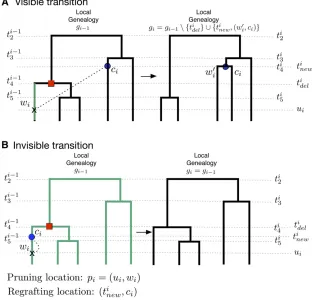
Figure 1 SMC9 hidden Markov model for inferring
population size trajectories, drawn according to Rasmussenet al.(2014) to highlight notation specific to our study. (A) Observed sequence data in a segment of lengthLfromfive individuals. Three loci are shown delimited by recombination breakpoints b1 and b2:
Only the derived mutations at polymorphic sites are shown. (B) Corresponding local genealogiesgifor each
locusi. Thefive sampled individuals are depicted as solid black circles. Local genealogies have a Markovian degree-1 dependency. Each intercoalescent time (the time interval between coalescent events denoted as open circles) provides information about past popula-tion size (number of solid gray circles at a given time point). Moving from left to right after recombination breakpointb1;the pruning locationp1is selected from
genealogyg0and the pruned branch is regrafted back
on the genealogy (solid blue circle). The coalescent event ofg0depicted as a solid red circle ing1is deleted. This creates the next genealogyg1:The
Methods: SMC9Calculations
Following notation similar to that in Rasmussenet al.(2014) (Table 1), a realization of the embedded SMC9chain consists of a set ofm
local genealogiesðg0;g1;...;gm21Þ;m21 recombination
break-points at chromosomal locationsðb1;b2;...;bm21Þ;andm21
pruning locations ðp1;p2;.. .;pm21Þ; where pi¼ ðui;wiÞ indi-cates the time of the recombination eventui and the branchwi where recombination happened in genealogygi21(Figure 1).
Ge-nealogyg0corresponds to the genealogy ofnsequences that
con-tains the set of timed ancestral relationships among the n
individuals for the chromosomal segmentð0;b1: Genealogygi corresponds to the genealogy of the same nsequences for the chromosomal segmentðbi;biþ1fori¼1;2;...;m22:Finally,
ti
jdenotes the time when two ofjlineages coalesce in genealogygi; measured in units of generations before present.
Using uppercase letters to denote random variables, the evolution of the SMC9 process along chromosomal segments is governed by a point process B¼ fBigi2ℕ that represents the random locations of recombination breakpoints. We use
Si¼Bi2Bi21; for i¼1;2;. . .;m; to denote the segment
lengths for each local genealogy, with S0¼B0¼0: Let
G¼ fGigi2ℕ be the chain that records the local genealogies, and let P¼ ðU;WÞ ¼ fðUi;WiÞgi2ℕ represent the chain that records the pruning locations (time and branch) onG. The se-quenceðGi;Pi¼ fUi;Wig;BiÞhas the following conditional in-dependence relation:
Pr
h
Gi¼gi;Ui#ui;Wi¼wi;Si#sgj;bjij¼201;uj;wjij2¼11
i
¼Pr½Si#sijgi21 (1)
3Pr½Ui#ui;Wi¼wijgi21 (2)
3Pr½Gi¼gijUi#ui;Wi¼wi;gi21: (3)
Thus, given a chain of local genealogies, pruning locations, and recombination breakpoints, the joint transition probabil-ity to a new genealogy, pruning location, and locus length can be expressed as the product of the locus-length probability conditioned on the current genealogy (Expression 1, above), the pruning location probability conditioned on the current genealogy (Expression 2, above), and the transition proba-bility of the new genealogy conditioned on the current gene-alogy and pruning location (Expression 3, above).
Complete data transition densities
Consider the chain of local genealogiesg¼ ðg0;g1;. . .;gm21Þ
with recombination breakpoints at b¼ ð0;b1;. . .;bm21Þ:
According to the SMC9process, thefirst local genealogyg0
follows the standard coalescent density
PrG0¼g0jNðtÞ
¼Y
n
j¼2 1
Nt0jexp
(
2
Z t0 j
t0 jþ1
A0ðtÞA0ðtÞ21dt
2NðtÞ
)
; (4)
where t0
nþ1¼0 and t0n,. . .,t02 are the set of coalescent
times in local genealogyg0:The piecewise constant function
AiðtÞdenotes the number of ancestral lineages present at time
tin genealogygi;that is,AiðtÞ ¼
Pn j¼1j1t2ðti
jþ1;t i jÞ;witht
i
1¼N:
Given a current local genealogygi21;the distribution of the
length Si¼Bi2bi21 of the current locus depends on the
current state of the SMC9chain through the local genealogy’s total tree lengthli21(the sum of all branch lengths ingi21)
and the recombination rate per site per generationr:
fðsijgi21;rÞ ¼rli21expf2rli21sig: (5)
At recombination breakpoint bi;a new local genealogygi is generated that depends on the previous local genealogygi21
and the population size trajectoryNðtÞ(Figure 1). To generate
giwefirst randomly choose a pruning locationpi(consisting of a pruning timeuiand a lineagewi) uniformly alonggi21:At
pruning locationpi;we add a new lineagew9iand coalesce it further in the past at timeti
newwith some lineage,ci(Figure 2). We then delete thewilineage’s segment from ui totdeli (the
coalescent time of lineagewi). The transition density to a new genealogy at recombination breakpointbiis then
Prpi¼ ðui;wiÞ;tnewi ;cijgi21;NðtÞ
¼Prpi¼ ðui;wiÞjgi21
Prtnewi ;cijui;gi21;NðtÞ
¼ 1
li21
1
Nti
new
exp
(
2
Z ti new
ui
Ai21ðtÞdt
NðtÞ
)
; (6)
whereli21 denotes the total tree length ofgi21:
Thisgenerativeprocessforlocalgenealogiescanresultinavisible transition, where a genealogygiis different fromgi21(Figure 2A),
or aninvisible transition, wheregiis identical togi21(Figure 2B).
An invisible transition (gi¼gi21) occurs when ci¼wi: Given the pruning location pi¼ ðui;wiÞ;an invisible transi-tion occurs whenTi
new2 ðui;tidelÞandCi;the random variable indicating the lineage that coalesces with lineagew9i;takes the valuewi:The probability of an invisible transition is given by
PrGi¼gi21jpi¼ ðui;wiÞ;gi21;NðtÞ
¼Pr
h
ui#Tnewi #tdeli ;Ci¼wijpi¼ ðui;wiÞ;gi21;NðtÞ
i
¼ Z ti
del
ui
1
NðtÞexp
(
2
Z t
ui
Ai21ðuÞdu
NðuÞ
)
dt:
Thus, the joint transition probability to an invisible event with pruning locationðui;wiÞ;givengi21;is
Pr½Gi¼gi21;pi¼ ðui;wiÞjgi21;NðtÞ
¼ 1
li21
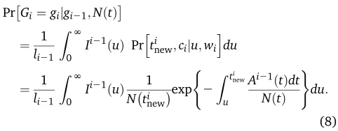
Transition densities averaged over unknown pruning locations
Even though we assume that local genealogies are known, to build inferential frameworks for sequence data in the future, we do not wish to make the same as-sumption about pruning locations. Thus, we average over pruning locations to obtain marginal transition den-sities between genealogies for both visible and invisible transitions.
Visible transitions: To compute the marginal visible
transition density to a new genealogy gi¼
fgi21∖ftidelg [ ftnewi ;ðw9i;ciÞgg;we need to average over all possible pruning locations pi¼ ðui;wiÞ along gi21: By
comparing the two genealogiesgi21andgiin Figure 2A, we know thatpicorresponds to the lineagewisome time along ð0;ti21
4 Þor, equivalently, alongð0;tidelÞ:In general,
comparison ofgi21 andgimay not provide complete in-formation to identify the lineage that was pruned. When the children of the node corresponding to tdel and the
children of the node corresponding totneware the same,
pruning different branches can lead to the same transi-tion. We enumerate all cases of incomplete information for visible transitions inSupporting Information,File S1, andFile S2.
We introduce a functionIi21ðtÞ;equal to the number of
possible lineages at time t where the pruning location along gi21 would produce a visible transition togi:Ii21ðtÞ is a piecewise constant function that takes the values in
f0;1;2g depending on whether the pruning location pi can happen in 0;1;or 2 branches at timet. In the example in Figure 2A,
Ii21ðtÞ ¼
1; if t20;ti421;
0; if t2t4i21;N
: (7)
For a general piecewise constant function Ii21ðtÞ;the
mar-ginal visible transition density to a new genealogy is
PrGi¼gijgi21;NðtÞ
¼ 1
li21
Z N
0
Ii21ðuÞ Pr
h
tinew;ciju;wi
i
du
¼ 1
li21
Z N
0
Ii21ðuÞ 1 Nti
new
exp
(
2
Z ti new
u
Ai21ðtÞdt NðtÞ
)
du:
(8)
Invisible transitions: To compute the marginal transition
probabilities for invisible events, we must average over all possible pruning locationspi:Consider the example in Figure 2B and choosing a pruning time (ui) alonggi21:To have an
Table 1 Notation for the SMC9model used in this work
Symbol Description
Parameters
r Recombination rate per site per generation
NðtÞ Effective population size trajectory with time measured in units ofN0generations
t Hyperparameter that controls the smoothness of the log-Gaussian process prior onNðtÞ
Notation specific to SMC9chain
L Length of observed sequences
bi Chromosomal location of theith recombination breakpoint
m No. local genealogies corresponding tom21 recombination events
siþ1¼biþ12bi Segment length for local genealogyi
gi Local genealogy for the segmentðbi21;bi
Notation specific to local genealogy
n Sample size or no. sequences
li Total tree length of local genealogygi
AiðtÞ Piecewise constant function of the number of ancestral lineages at timetin local genealogyg
i ti
j Coalescent time in genealogygiwhen two ofjlineages coalesce.Aiðtij2Þ ¼j;AiðtjiþÞ ¼j21:
ti¼ ðti
n;tn2i 1;. . .;t2iÞ Vector of coalescent times of genealogygi
pi¼ ðui;wiÞ Pruning location along local genealogygi
ui Time when the recombination event happened along the height of the genealogygi
wi Lineage on genealogygi21where the recombination event happened
wi9 New lineage added on genealogygiwhere the recombination event happened
ti
new Coalescent time in genealogygiwhen the lineagewicoalesces
ti
del Coalescent time in genealogygi21that no longer exists in genealogygi
ci Lineage on genealogygithat coalesces with lineagewi9
Fi
j;k No. free lineages in local genealogygithat do not coalesce in the time intervalðtjþi 1;tkiÞ
IiðtÞ Piecewise constant function that takes values inf0; 1; 2gindicating no. ancestral lineages
at timetin genealogygiwhere the pruning event would produce a visible transition togiþ1
Discretization
d No. change points at whichNðtÞis estimated
invisible transition, the coalescing branch Ci must be the same pruning branch Wi:In Figure 2B the new coalescent time Ti
new can happen along five lineages in the interval ð0;ti21
5 Þ;three lineages in the intervalðt5i21;ti421Þ;and two
lineages in the intervalðti21
4 ;ti321Þ:To generalize this
calcu-lation, we introduce the quantity Fi
j;k with n$j$k$2; which denotes the number of lineages ingithat arefree(do not coalesce), in the time segment ðti
jþ1;tkiÞ;with tinþ1¼0:
The time interval ðti
jþ1;tikÞ includes the interval of pruning
ðti
jþ1;tijÞup to the interval of self-coalescenceðtikþ1;tkiÞ:Thus, if the pruning time happens at timeUi2 ðtijþ1;tijÞ;an invisible transition with new coalescent timeTi
new2 ðtkiþ1;tikÞcan hap-pen alongFi
j;kfree lineages.
In Figure 2B,uihappened in the time intervalð0;ti521Þ:If
the new coalescent timeTi
newhappens in the intervalðui;ti521Þ
along the same (unknown) pruning branch, then this invisi-ble transition has probability
Pr
h
Gi¼gi21;Tnewi 2
ti21
6 ;ti521ui;gi21;NðtÞ
i
¼Fi52;51
Z ti21 5
ui
1
NðtÞexp
(
2
Z t
ui
Ai21ðuÞdu
NðuÞ
)
dt;
withF5;5¼5:
Now consider the same example of Figure 2B but with an unknown pruning timeui:The joint event where recombina-tion occurs at pruning time Ui2 ðt6i21;t5i21Þ and coalescent
time Ti
new occurs in the intervalðti621;ti521Þ and this results
in an invisible transition has probability
Pr
h
Gi¼gi21;Ui2
t6i21;t5i21;Tnewi 2t6i21;ti521gi21;NðtÞ
i
¼F
i21 5;5
Rti21 5
ti21 6
Rti21 5
ui ð1=NðtÞÞexp
n
2Rt ui
Ai21ðuÞduNðuÞodtdu
i li21
(9)
¼F
i21 5;5P5i2;51
li21 ;
(10)
wherePi21
5;5 denotes the double integral expression in
Equa-tion 9 for ease of notaEqua-tion.
An invisible transition would also result ifUi2 ðti621;t
i21
5 Þ
and Ti
new2 ðti521;ti421Þ along the same (unknown) pruning
branch; in Figure 2B, this can happen along three lineages, soFi21
5;4 ¼3 and this event has probability
Pr
h
Gi¼gi21;Ui2
t6i21;t5i21;Tnewi 2
t5i21;t4i21gi21;NðtÞ
i
¼
Fi21 5;4
Rti21 5
ti21 6
exp
2Rti21 5
ui
Ai21ðuÞduNðuÞ
li21
3
Z ti21 4
ti21 5
1
NðtÞexp
(
2
Z t
ti21 5
Ai21ðuÞdu NðuÞ
)
dtdui
¼F
i21 5;4Pi52;41
li21 :
If we continue considering the cases where Ui2 ðti621;ti521Þ
andTi
new2 ðti421;t3i21ÞorTnewi 2 ðt3i21;ti221Þ;we haveFi52;31¼2
Figure 2 Schematic representation of SMC9
transi-tions given a recombination breakpoint at locationbi
(indicated as an arrow in each panel). (A) Visible tran-sition. We uniformly sample the pruning location pi
fromgi21at timeuialong some branchwi;and we
add a new branchwi9atuiand regraft it (dashed black
line). The new branchwi9coalesces with some branchci
at time tinew: We then delete branchw
i and the
co-alescent timeti
delto generate genealogygi:Any
prun-ing time along the branchwi(shown in green) would
have produced the same visible transition fromgi21to
gi: (B) Invisible transition. We uniformly sample the
pruning location pi¼ ðui;wiÞ; add a new branchwi9
atui;and regraft it. The new branchwi9coalesces with
itself (dashed black line), that is,Ci¼wi;and then the
segmentðui;tdeli Þofwiis deleted. IfCi¼wi;any
andFi21
5;2 ¼0:Then, the joint probability of an invisible event
andUi2 ðt6i21;ti521Þis
Pr
h
Gi¼gi21;Ui2
ti6;ti5gi21;NðtÞ
i ¼
P5
k¼2Fji;2k1Pij2;k1 li21 :
For the cases whenUi2 ðtji2þ11;t
i21
j Þ and the new coalescent timeTi
newfalls in another coalescent intervalðt
i21
kþ1;t
i21
k Þ;we need to compute the following: the joint probability of
Ui2 ðtijþ211;t
i21
j Þand no coalescence in the intervalðui;tij21Þ;
1
li21
Qij21¼
1
li21
Z ti21 j
ti21 jþ1
exp
(
2
Z ti21 j
ui
Ai21ðuÞdu NðuÞ
)
dui;
the probability of no coalescence in any of the intermediate coalescent intervalsðti21
lþ1;til21Þ;
qil21¼exp
(
2
Z ti21 l
ti21 lþ1
Ai21ðuÞdu NðuÞ
)
;
and the probability of coalescing atTi
new2 ðtik2þ11;tki21Þ;
12qik21:
Then,
1
li21
Pij2;k1¼ 1 li21
Qji21qij2211qji2212. . .qik2þ11
12qik21
represents the probability that the pruning location iswiat timeUi2 ðtij2þ11;tji21Þand the new lineagew9icoalesces at time
Ti
new2 ðtki2þ11;t
i21
k Þwith lineageci¼wi:Overall, the marginal transition probability to an invisible event is
Pr½Gi¼gi21jgi21;NðtÞ
¼ Z ti21
2
0
PrGi¼gi21;uijgi21;NðtÞ
dui
¼X
n
j¼2 Pr
h
Gi¼gi21;Ui2
tjiþ211;tji21gi21;NðtÞ
i
¼ 1
li21
Xn
j¼2
Xj
k¼2
Fji;2k1Pij2;k1: (11)
The likelihood of the embedded SMC9chain
Instead of having a complete realization of the embedded SMC9 chain ofmlocal genealogiesg0;. . .;gm21 and pruning
loca-tionsp1;. . .;pm21at recombination breakpointsb1;. . .;bm21;
we assume that our data (unless otherwise noted) consist only of m local genealogies at recombination breakpoints from a chromosomal segment of lengthL(including visible and in-visible events). Note that our observed data are not sequence data. More specifically, our observed data are
Y¼ðg0;0Þ;ðg1;b1Þ. . .;ðgm21;bm21Þ;sm¼L2bm21
: (12)
Then, the observed data likelihood is
LobsðY;NðtÞ;rÞ ¼Pr
h
g0jNðtÞ
i" Ym22
i¼0 Pr
h
giþ1jgi;NðtÞ
i# zfflfflfflfflfflfflfflfflfflfflfflfflfflfflfflfflfflfflfflfflfflfflfflfflfflfflfflfflfflfflfflffl}|fflfflfflfflfflfflfflfflfflfflfflfflfflfflfflfflfflfflfflfflfflfflfflfflfflfflfflfflfflfflfflffl{factors that depend on NðtÞ
3hðL2bm21jgm21;rÞ
" Y
m22
i¼0
f½siþ1jgi;r
#
|fflfflfflfflfflfflfflfflfflfflfflfflfflfflfflfflfflfflfflfflfflfflfflfflfflfflfflfflfflfflfflfflfflffl{zfflfflfflfflfflfflfflfflfflfflfflfflfflfflfflfflfflfflfflfflfflfflfflfflfflfflfflfflfflfflfflfflfflffl}
factors that depend on r
;
(13)
where hðL2bm21jgm21;rÞ is the survival function in state
gm21: Equation 13 is factored into terms that depend on
NðtÞalone and ones that depend onralone. The terms that depend onr, given by Equation 5, depend on the data only through total tree lengths l0;. . .;lm21 and locus lengths
s1;. . .;sm21;L2bm21:By the factorization theorem for suffi
-cient statistics, local tree lengths l0;. . .;lm21 and locus
lengths s1;. . .;sm21;L2bm21 are sufficient for inferring r.
Moreover, recombination locations b0;b1;. . .;bm21 do not
provide information aboutNðtÞ:
Methods: Inference
Current coalescent-based methods that infer a population size trajectoryNðtÞ from whole-genome data assumeNðtÞ
is a piecewise constant function with change points
x1¼0,x2,. . .,xd (Li and Durbin 2011; Sheehanet al. 2013; Rasmussen et al.2014; Schiffels and Durbin 2014). That is,
NðtÞ ¼X d
i¼1
Ni1t2ðxi21;xi: (14)
Equation 14 presents two challenges. Thefirst challenge lies in the specification of the change points: the narrower an interval is, the higher the probability that we do not observe coalescent times in that interval; further, the fewer observed coalescent times in an interval, the greater the uncertainty is of the estimate Nbi (if the estimate even exists). The second chal-lenge lies in the specification of the time windowð0;xdÞ:if
xdis set too far in the past, we might not have enough data to accurately estimateNðtÞforxd#t,N:
To solve the first challenge, Li and Durbin (2011) and Rasmussenet al.(2014) distribute thedchange points evenly on a logarithmic scale,
xj¼1
k
(
exp
j
dlogð1þkxdÞ
21
)
; (15)
and setl¼
n
2
However, this equation is not directly
ap-plicable here because we use all coalescent events for inference.
In the following sections, we first present our Bayesian nonparametric method and then develop a maximum-likelihood method under a piecewise constant trajectory so we can directly compare an EM-based method to our Bayesian nonparametric method.
Gaussian-process-based Bayesian nonparametric estimation of N(t)
For our Bayesian methodology, we assume the log-Gaussian process prior on the population size trajectory,
NðtÞ ¼expfðtÞ; fðtÞ GPð0;CðtÞÞ; (16)
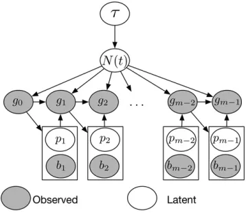
where GPð0;CðtÞÞ denotes a Gaussian process with mean function 0 and inverse covariance function C21ðtÞ ¼tC21 with precision parametert. For computational convenience, we use Brownian motion as our prior forfðtÞsince its inverse covariance matrix is sparse. We place a Gamma prior on the precision parametert,tGða;bÞ:Assuming that recombi-nation rate r is known, the posterior distribution of model parameters (Figure 3) is then
Pr½NðtÞ;tjg0;. . .;gm21
}
Pr½g0jNðtÞ3 Ym22 i¼0
Pr
giþ1jgi;NðtÞ
Pr½NðtÞjtPrðtÞ: (17)
Thefirst two factors on the right side of Equation 17, detailed in Equations 8 and 11, involve integration over NðtÞ; an infinite-dimensional random function (Equation 16). We approximate the integral
Z b
a dt NðtÞ¼
Z b
a
exp½2fðtÞdt;
by the Riemann sum over a partition of the integration in-terval. That is,
Z b
a
exp
h
2fðtÞ
i
dtX k
j¼i
exp
h
2f*
j
i
Dj; (18)
for xi,a,xiþ1,. . .,xk21,b,xk; Di¼xiþ12a; Dk¼b2xk21;andDj¼xjþ12xjfori,j,k21:fj*is a rep-resentative value offðtÞin the intervalðxj;xjþ1Þ;in our
imple-mentation, we set f*
j ¼fðx*jÞ with xj*¼ ðxjþxjþ1Þ=2: This
way, we discretize our time window indevenly spaced seg-ments x1 ¼0,x2,. . .,xd; with xd¼maxðt01;. . .;tm121Þ;
the maximum time to the most common ancestor observed in the sequence of local genealogies, and approximateNðtÞby a piecewise linear function evaluated atðx*
1;x*2;. . .;x*dÞ: We condition on the set ofmlocal genealogiesg0;. . .;gm21
(assuming pruning locations are not known) to generate pos-terior samples for the vector f*¼ ½logNðx*
1Þ;. . .;logNðx*dÞ and t and use these posterior samples to infer NðtÞ at
t2 ðx*
1;. . .;x*dÞ;wherex
*
i ¼ ðxiþxiþ1Þ=2:Updating the
vec-torfandtseparately is not recommended because of their strong dependency (Lanet al.2015). Therefore, we update (f;tÞ jointly in an MCMC sampling algorithm, using splitHMC (Shahbabaet al.2014; Lanet al.2015). splitHMC updates all model parameters jointly and it can be extended to a full inferential framework that is directly applicable to sequence data. The splitHMC method relies on Hamiltonian dynamics to propose a new state of the model parameters jointly with a higher acceptance rate than simple methods such as random-walk Metropolis (Neal 2009). splitHMC relies on our ability to calculate the log-likelihood of the observed data and the gradient vector of the log-likelihood (i.e., the score function). The log-likelihoods of the observed data are approximated via sums of the form in Equation 18. We approximate the score function=LobsðY;f*Þwith respect
tof* by applying Fisher’s identity,
=LobsðY;f*Þ ¼Ef*½=LcðYc;f*ÞjY;
where, at each iteration in the MCMC, expectation is calcu-lated using the current value off* (seeAppendix).
Alternatively, one can updateNðtÞin the MCMC algorithm, using the elliptical slice sampler (Murrayet al.2010) with afixed value oft(perhaps estimated from previous studies or from a preliminary run from the split Hamiltonian Monte Carlo algorithm). The advantage of using the elliptical slice sampler over the split Hamiltonian Monte Carlo is purely computational (the elliptical slice sampler does not require calculation of the score function).
Maximum-likelihood estimation of N(t) with measures of uncertainty
We assume that the population size trajectoryNðtÞis defined as in Equation 14. The standard coalescent density (Equation
Figure 3 Structure of our Bayesian model for inferring population size trajectories from a realization of the SMC9 process at recombination breakpoints. Hyperparameter t controls the smoothness of the log-Gaussian process prior onNðtÞ:Local genealogies depend onNðtÞand form a Markov chain of degree 1. Given the current local genealogygi21;
we sample the location of the new recombination breakpoint bi and
a pruning locationpion genealogygi21:The new genealogygidepends
4) and the transition densities defined in Equations 8 and 11 are tractable, so calculation of the likelihood (Equation 13) is tractable. However, maximization of the likelihood function cannot be performed analytically because pruning locations are missing. We implement an EM algorithm (Dempster
et al. 1977) to find the maximum-likelihood estimator of N¼ ðN1;. . .;NdÞ: The complete data Yc for inferring NðtÞ
are then the set of local genealogies g0;. . .;gm21 and the
set of pruning locationsp1. . .;pm21:For the invisible
transi-tions, we also need to know the new coalescent times
fti
newgi2I ;whereI⊂f1;2;. . .;m21gdenotes the set of
in-dexes of invisible transitions.
The complete data log-likelihood is then
LcðYc;NÞ:¼logPr½g0jNðtÞ (19)
þX
m21
i¼1
log Prpi¼ ðui;wiÞ;tnewi ;cijgi21;NðtÞ
:
The EM algorithm starts by initializing the population size trajectory to a piecewise constant function with change points
x1;. . .;xdwith arbitrarily chosen vectorN0:At thekth itera-tion of the algorithm we set
Nk¼arg max
N ENk21½LcðYc;NÞjY: (20)
The conditional expectation in Equation 20 is conditional on the observed data Y defined in Equation 12. Let xi¼ fxi
1;
xi
2;. . .;xdiþn21gbe the ordered set of time points corresponding
to the change pointsx1;. . .;xdand the coalescent time pointsti of local genealogyi. If the transition fromgitogiþ1 is visible,
we replace thejth time pointxi
j bytinewþ1;wherejcorresponds
to the index such thatxi
j21,tinewþ1#xij:For ease of notation, we denote the number of time intervalsjxijbyD¼dþn22:Let
a0j ¼
1; if x0
jþ1¼t0k; for k¼2;. . .;n;
0; otherwise;
be an indicator function that takes the value of 1 when thejth interval contains a coalescent time of thefirst genealogyg0:
Then, the log density of thefirst genealogy is
log Pr½g0jNðtÞ ¼ 2X D
j¼1 n
a0
j logN x0 jþ1 o 2X D j¼1
A0x0
jþ1 h
A0x0
jþ1
21ix0
jþ12x0j
exph2logNx0
jþ1 i 2 8 > < > : 9 > = > ;: (21) Let
zij¼
1; if xi
j,tinewþ1#xjiþ1; 0; otherwise;
be an indicator function that takes the value of 1 when the new coalescent time of genealogy ihappens in the
corre-sponding time intervalðxi
j;xijþ1Þ;and let the adjusted
inter-val length be
Di j¼ 8 > > > > > > > > > > > > < > > > > > > > > > > > > :
xijþ12xji; if uiþ1,xji; and xijþ1,tinewþ1
ðafter pruning and before coalescenceÞ; xi
jþ12uiþ1; if xij,uiþ1,xijþ1#tinewþ1
ðbefore coalescence with pruning adjustmentÞ; tiþ1
new2uiþ1; if xij,uiþ1,tinewþ1,xjþ1
ðadjustment for pruning and coalescenceÞ; tiþ1
new2xij; if uiþ1,xji,tinewþ1,xijþ1
ðafter pruning with coalescence adjustmentÞ; 0; otherwise:
Then, the augmented transition density can be expressed as
log Prpi¼ ðui;wiÞ;tnewi ;cijgi21;NðtÞ
¼log Prhpi¼ ðui;wiÞ;ti
new;ci;zi;Dijgi21;NðtÞ
i
¼ 2logli212
P
Dj¼1
zi21
j logN
xi21
jþ1
2
P
Dj¼1
n
Ai21xjiþ211Dij21exp
2logNxjiþ211o; (22)
whereziandDi
are the vectors withzi jandD
i
jelements. For the EM algorithm we need to compute the conditional expected vectors E½zi
jY and E½D i
jY: The details of these calculations are in theAppendix.
We use the Fisher information matrix to compute approx-imate standard errors of logN
^
and use these standard errors together with asymptotic normality of maximum-likelihood estimators to produce confidence intervals for log population size piecewise trajectories. We compute the observed Fisher information matrix following Louis (1982),^
IY
^
N¼E^N
2H
^
Lc
Yc;N
^
Y2E^N h
=Lc
Yc;N
^
=Lc
Yc;N
^
9Yi;where=LcðYc;N
^
Þis the gradient andHLcðYc;N^
Þis theHes-sian of the complete-data log-likelihood with respect to logN: This requires the calculation of conditional cross-product means and conditional second moments described inFile S7.
Data availability
The R code for all simulation studies and analysis of se-quence data conducted in this article are publicly available athttp://ramachandran-data.brown.edu/.
Results
We simulated 1000 local genealogies of 2, 20, and 100 individuals from each of the three different demographic models described in Table 2, using MaCS (Chen et al.
We compared our point estimates with the truth for each demographic model, using the sum of relative errors (SRE),
SRE¼X
K
i¼1
N
^
ðxiÞ2NðxiÞNðxiÞ ; (23)
where N
^
ðxiÞ is the estimated population size trajectory at time xi: We compute SRE at equally spaced time pointsx1;. . .;xK: Second, we compute the mean relative width (MRW) as
MRW¼X
K
i¼1
N
^
upðxiÞ2N^
lowðxiÞKNðxiÞ ; (24)
where N
^
upðxiÞ corresponds to the 97:5% upper limit and^
NlowðxiÞ corresponds to the 2:5% lower limit of N
^
ðxiÞ: For EM estimates, ½N^
lowðxiÞ;N^
upðxiÞ corresponds to the 95% confidence interval estimated using the observed Fisher in-formation; for Bayesian GP estimates,½N^
lowðxiÞ;N^
upðxiÞ cor-responds to the 95% Bayesian credible interval (BCI) of^
NðxiÞ:To measure how well these intervals cover the truth, we compute the envelope measure (ENV) in the following way:
ENV¼
PK i¼1I
^
NupðxiÞ#NðxiÞ#N
^
lowðxiÞ
K : (25)
We compute SRE, MRW, and ENV for K¼150 at equally spaced time points.
For our Bayesian GP estimates, we estimate NðxiÞ at
d¼100 time points, unless stated otherwise.
The parameters of the Gamma prior on the GP precision parametertwere set toa¼b¼0:001;reflecting our lack of prior information about the smoothness of the population size trajectory.
For our EM estimates, we used different discretizations based on Equation 15 and varying the number of change points dand kover thefixed intervalð0;xdÞwith xd set to be the maximum observed coalescent time. For the cases where we consider only one genealogy (m¼1), the EM ap-proach becomes standard maximum-likelihood estimation.
We summarize our posterior inference and compare our Bayesian GP method to the EM method in Figure 5, Figure 6, and Figure 7. The population size trajectory is log-transformed
for ease of visualization and for direct comparison with other methods (Mininet al.2008; Palacios and Minin 2013).
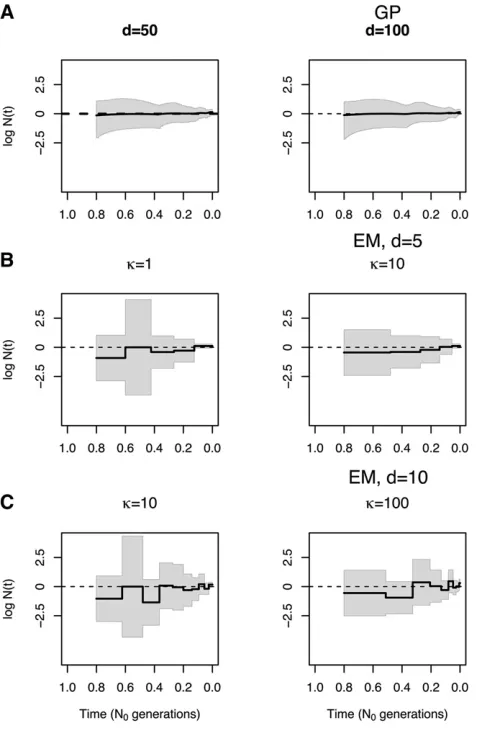
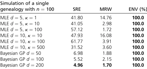
Sensitivity of EM estimates of N(t) to discretization
In Figure 4, we show our Bayesian GP and EM estimates of a constant population size trajectory from a single genealogy of 100 individuals with different discretizations. Wefind that our Bayesian GP point estimates depicted in Figure 4A re-cover the truth (dashed line) almost perfectly with less un-certainty than the EM (Figure 4, B and C). Comparing our Bayesian GP estimates with different discretizations [50, 100, and 200 equally spaced time points (Figure 4A)], wefind that increasing the number of time points improves inference (Table 3) but that the differences between estimates among the three discretizations are marginal (Figure 4A). In con-trast, we show that different grid definitions alter the EM estimates (Figure 4B). It is not clear how to define a good strategy for the definition of the grid for the EM method, even for the simple model of constant population size. For exam-ple, increasingkfrom 100 to 500 with 5 change points (Fig-ure 4B) does not improve estimation. Increasing the number of change points does not necessarily improve the estimates either, for example, increasing the number of change points from 5 to 10 fork¼10 (Figure 4, B and C). EM grid sensi-tivity is persistent even when the number of genealogies increases;Figure S2inFile S4shows that the best definition of change points when our data consist of 1000 local geneal-ogies of 100 individuals is 10 evenly distributed change points.
Comparing methods for estimating N(t)
Figure 5 shows the estimated population size trajectories when the number of samples is two for the three different demographic scenarios and varying the number of local genealogies (100, 500, and 1000 local genealogies). For constant and exponential growth, our EM method assumes a piecewise constant trajectory of 10 change points (d¼10) and k¼1; using Equation 15 (similar to Li and Durbin 2011 and Rasmussenet al.2014). For the bottleneck sce-nario, some of the intervals did not have coalescent events; hence, for this case we assumed a piecewise constant trajec-tory of 5 change points (d¼5) andk¼1 for constructing our EM estimates. We show the boxplots of the time to the most recent common ancestor (TMRCA) at the bottom of
Table 2 Simulated demographic scenarios
Demographic model N(t)
Constant population size NðtÞ ¼1
Exponential growth followed by constant size NðtÞ ¼
1; for t2 ð0;0:1Þ;
exp½210ðt20:1Þ; for t2 ð0:1;NÞ:
Population bottleneck NðtÞ ¼
8 < :
1; for t2 ð0;0:3Þ;
0:1; for t2 ð0:3;0:5Þ; 1; for t2 ð0:5;NÞ:
each plot in Figure 5, which indicate the uncertainty expected in our estimates.
Both approaches, EM and Bayesian GP, show narrower confidence and credible intervals at the center of the distri-bution of the TMRCA, particularly during the bottleneck in Figure 5C.
For the constant population size model in Figure 5A, our Bayesian GP considerably outperforms our EM estimates. This is not surprising since a priori logNðtÞ has mean 0 in our Bayesian approach (Equation 16). Moreover, EM confi -dence intervals cover the truth only30% of the time, while the GP method covers 100% of the truth (Table 4A). Despite placing a mean-0 prior on logNðtÞ;the Bayesian GP method accurately recovers sudden changes as shown in the bottle-neck scenario. Although our Bayesian GP prior on logNðtÞis Brownian motion (which is not differentiable at any point), our Bayesian GP recovers smooth curves (Figure 5B).
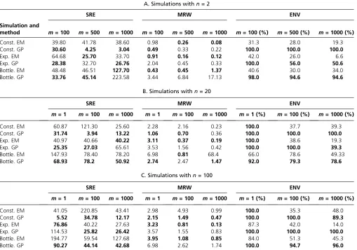
Table 4A shows the performance statistics for the esti-mates of NðtÞ in Figure 5. In general, our Bayesian GP has wider credible intervals than the EM confidence intervals but these credible intervals cover the true trajectory better than the EM confidence intervals in all cases (MRW and ENV in Table 4). Our Bayesian GP estimates also generally have smaller sums of relative errors (SRE in Table 4). Under the
bottleneck scenario, our Bayesian GP produces greater sums of relative errors than does the EM, but our Bayesian GP estimates recover the truth more accurately than the EM during the bottleneck.
Figure 6 and Figure 7 show our estimates when n¼20 andn¼100 (Table 4, B and C, gives performance statistics). In general, our GP-based estimates have smaller SRE and larger ENV than the EM-based estimates and hence, the MRW is usually wider in the GP-based estimates, accurately reflecting the uncertainty of the estimates. As expected, in-creasing the number of loci (m) generally decreases the width of the confidence and credible intervals of our mates (MRW). Although this is generally true for EM esti-mates as well, EM estiesti-mates have very low coverage of the truth (MRE in Table 4) when the number of loci increases.
Sampling more individuals vs. sequencing more loci
Figure 5, Figure 6, and Figure 7 show our estimates for
n¼2; 20;and 100 sampled individuals across varying num-bers of loci. Performance of EM estimates depends strongly on the definition of the grid, so we focus here on the Bayesian GP estimates. We find that increasing the number of loci decreases uncertainty of our estimates and allows us to infer
NðtÞfarther back in time. Increasing the number of samples
does not necessarily increase the performance of our GP esti-mates (File S6). For example, under the bottleneck scenario, we are able to detect the bottleneck fairly accurately even for two samples with m¼1000 local genealogies. This is be-cause most TMRCAs observed under the bottleneck scenario occur during the bottleneck (Figure 5, Figure 6, and Figure 7), regardless of the sample size. In contrast, in our exponen-tial growth scenario, increasing the number of samples from
n¼2 to n¼100 improves accuracy: point estimates are
closer to the truth (SRE in Table 4, A–C) and credible inter-vals cover the truth completely (ENV of 100%).
Sequential Tajima’s genealogies are sufficient statistics
under the SMC9
Under the SMC9, marginally at each locus along the chro-mosome, a local genealogy is a realization of Kingman’s
n-coalescent (Kingman 1982), a continuous-time Markov chain taking its values in the setKnof sequences of partitions of the label setf1;2;. . .;ngA local genealogygofn individ-uals includes labeled topology Kn and coalescent times t¼ ðtn;. . .;t2Þ:The state space of a local genealogy is then G ¼ Kn5ℝþn21; and the cardinality of the set Kn is
n!ðn21Þ!=2n21:However, only the set of ordered coalescent
times carries information aboutNðtÞ:For a single locus, the set of coalescent times provides sufficient statistics for infer-ringNðtÞ(seeProofin theAppendix). A natural question that follows is whether the coalescent times corresponding to the set of local genealogies are sufficient statistics for inferring
NðtÞunder the SMC9model. Wefind that the sufficient sta-tistics for inferring NðtÞunder the SMC9model are the co-alescent times, when taken together with localranked tree shapes(tree with no labels but ranked coalescent events). For a single locus, the set of coalescent times together with the ranked tree shape corresponds to a realization of Tajima’s
Table 3 Summary statistics for simulation results depicted in Figure 4
Simulation of a single
genealogy withn¼100 SRE MRW ENV (%)
MLEd¼5;k¼1 41.80 14.76 100.0
MLEd¼5;k¼10 41.05 2.98 100.0
MLEd¼5;k¼100 57.12 1.72 100.0
MLEd¼10;k¼10 47.93 16.08 100.0
MLEd¼10;k¼100 61.77 3.91 100.0
MLEd¼10;k¼500 31.52 3.60 100.0
Bayesian GPd¼50 6.98 1.88 100.0
Bayesian GPd¼100 5.52 2.15 100.0
Bayesian GPd¼200 4.96 1.70 100.0
SRE is the sum of relative errors (Equation 23), MRW is the mean relative width of the 95% BCI (Equation 24), and ENV is the envelope measure (Equation 25). Values in boldface type indicate best performance.
n-coalescent. Tajima’sn-coalescent (Tajima 1983) is a contin-uous-time Markov chain taking its values in the set Hn of ranked tree shapes [also called histories, evolutionary rela-tionships, or vintaged and sized coalescent (Sainudiinet al.
2014)]. The state space of Tajima’s local genealogy is then
GT¼ H
n5ℝþn21; and the cardinality of the set Hn corre-sponds to the sequence of Euler zigzag numbers whosefirst 10 elements are 1; 1; 1; 2; 5; 16; 61; 272; 1385; 7936 (Disanto and Wiehe 2013). The probability of getting a particu-lar type of ranked tree shapeHnofnsamples (Tajima 1983) is given by
PðHnÞ ¼ 2 n2c21
ðn21Þ!; (26)
wherecis the number ofcherries, defined as branching events that lead to exactly two leaves.
We defined transition densities in terms of coalescent times andFi;jquantities (seeMethods: SMC9calculations). The set of allFi;jquantities from a local genealogy forms a triangular ma-trix: anFmatrix. We show that (i)Fmatrices are in bijection
with ranked tree shapes and (ii) the set of local Tajima’s gene-alogies has sufficient statistics for inferringNðtÞunder the SMC9 model (seeAppendix). These observations are crucial for infer-ringNðtÞfrom sequence data directly. Coalescent-based infer-ence from sequinfer-ence data relies on marginalization over the hidden state space of genealogies. In the Appendix, we show that the state space needed is the space of local Tajima’s gene-alogies, as opposed to the space of local Kingman’s genealogies. Forn¼10 sequences, there are 2;571;912;000 possible la-beled topologies while only 7936 possible ranked tree shapes.
Application to human data
We applied our method to a 2-Mb region on chromosome 1 (187,500,000–189,500,000) with no genes fromfive Yorubans from Ibadan, Nigeria (YRI) andfive Utah residents of central European descent (CEU) from the 1000 Genomes pilot project (1000 Genomes Project Consortium 2012) and previously ana-lyzed for the same purpose (Sheehan et al. 2013). We used
ARGweaver (Rasmussenet al.2014) to obtain a sample path of local genealogies for the two populations (YRI and CEU). The
Table 4 Summary of simulation results depicted in Figure 5
A. Simulations withn= 2
SRE MRW ENV
Simulation and
method m= 100 m= 500 m= 1000 m= 100 m= 500 m= 1000 m= 100 (%) m= 500 (%) m= 1000 (%)
Const. EM 39.80 41.78 38.60 0.98 0.26 0.08 31.3 28.0 19.3
Const. GP 30.60 4.25 3.04 0.49 0.33 0.22 100.0 100.0 100.0
Exp. EM 64.68 25.70 33.70 0.91 0.16 0.12 42.0 26.0 6.6
Exp. GP 28.38 32.70 26.76 2.04 0.45 0.33 100.0 56.0 50.6
Bottle. EM 48.48 46.51 127.70 0.43 0.45 1.37 40.6 30.0 34.0
Bottle. GP 33.76 45.14 223.58 3.44 6.84 17.13 98.0 94.6 94.6
B. Simulations withn= 20
SRE MRW ENV
m= 1 m= 100 m= 1000 m= 1 m= 100 m= 1000 m= 1 (%) m= 100 (%) m= 1000 (%)
Const. EM 60.87 121.30 25.60 2.28 2.16 0.23 100.0 37.7 39.3
Const. GP 31.74 3.94 13.22 1.06 0.70 0.36 100.0 100.0 100.0
Exp. EM 40.97 40.66 40.22 3.11 0.37 0.19 100.0 38.6 19.3
Exp. GP 25.35 27.03 65.61 3.53 1.56 0.42 100.0 100.0 39.3
Bottle. EM 147.93 78.40 78.20 6.98 0.81 68.4 66.0 78.6 49.33
Bottle. GP 68.93 78.2 50.92 2.74 2.47 1.47 92.0 79.3 78.6
C. Simulations withn= 100
SRE MRW ENV
m= 1 m= 100 m= 1000 m= 1 m= 100 m= 1000 m= 1 (%) m= 100 (%) m= 1000 (%)
Const. EM 41.05 220.85 43.41 2.98 4.93 0.99 100.0 35.3 48.0
Const. GP 5.52 34.78 12.17 2.15 1.49 0.47 100.0 100.0 89.3
Exp. EM 76.86 40.22 27.63 3.23 0.81 0.13 87.3 42.0 14.0
Exp. GP 114.53 25.82 26.42 3.57 1.55 0.83 100.0 100.0 100.0
Bottle. EM 194.77 59.54 127.68 3.95 1.08 0.85 84.0 51.3 45.3
Bottle. GP 90.27 44.14 42.68 6.98 2.62 1.74 100.0 94.7 96.0
parameters used were 200 change points, a mutation rate of m¼1:2631028;and a recombination rate ofr¼1:631028
(Rasmussen et al.2014) (File S5). We note thatARGweaver assumes the SMC process and our method assumes the SMC9 process. Moreover, our inference is based on a single sample of the SMC process with known pruning times. OurARGweaver set of local genealogies is discretized at 200 time points and our GP-based inference is influenced by this discretization. In Figure 8 we show our estimates of past Yoruban (in blue) and European population sizes (in green). The two population size trajectories experience a series of bottlenecks and overlap until100 KYA, assuming a diploid reference population size ofN0 = 10,000
and a generation time of 25 years. In Figure 8 we recover an out-of-Africa bottleneck that starts100 KYA and ends30 KYA in the European population. These results are consistent with pre-viously published results (Gronau et al.2011; Li and Durbin 2011; Rasmussenet al. 2011; Sheehanet al. 2013; Schiffels and Durbin 2014). In File S5,Figure S4A, we show the esti-mates of logNðtÞinstead ofNðtÞand time measured in units of
N0generations (as in Figure 5, Figure 6, and Figure 7). We note
that this two-step procedure of inferring local genealogies with
ARGweaver and then using our method introduces biases and ignores genealogical uncertainty. InFile S5, we correct for some of the bias caused by using this two-step procedure and show that our inferred population size trajectory remains valid for the recent past.
Assessing the effect of using genealogies inferred with ARGweaver
We simulated sequence data, usedARGweaver for inferring a set of local genealogies, and used our method on those genealogies to obtain estimates of logNðtÞ:To this end, we took the sequences of the first 1000 local genealogies of
n¼20 individuals simulated with MaCS as described in sec-tion 3 of File S5. We then generated the sequence lengths (si;for the locus corresponding togi21) as in Equation 5,
si Exponentialðr3li213N0Þ;
whereli21is the tree length ofgi21in units ofN0generations
andN0is the current population size. In our simulations, we
setN0¼20;000;r¼1:831028:To simulate sequence data
Figure 6 Inference of population size
of lengthsi over genealogygi21;we used Seq-Gen (Rambaut
and Grassly 1997) implemented in the R package phyclust (Chen 2011) from the Jukes–Cantor mutation model (Jukes and Cantor 1969) with mutation rate m¼231:831028:
We then usedARGweaver to infer a sample of local genealogies with the same corresponding parameters and with 200 change points for discretization of time. Figure 9 shows three estima-tions of effective population size trajectories for our three sim-ulation scenarios. Figure 9, A–C, left, shows our GP-based estimates from 1000 simulated genealogies from MaCS; Figure 9, A–C, center, shows our GP-based estimates from a realization of local genealogies obtained fromARGweaver; and Figure 9, A–C, right, shows our GP-based estimates correcting the num-ber of lineages used in our calculations, replacing AiðtÞ by
AiðtÞ21 in our likelihood calculations. Wefind that our esti-mates are not only noisier using this approach but also biased.
Discussion
In this article, we propose a Gaussian-process-based Bayesian nonparametric method for estimating effective population
size trajectories NðtÞ from a sequence of local genealogies, accounting for recombination. Under a variety of simulated demographic scenarios and sampling designs, our method recovers the truth with better precision and accuracy than a maximum-likelihood approach (Figure 5, Figure 6, and Fig-ure 7). We apply our method to genealogies estimated using
ARGweaver (Rasmussenet al.2014) for European and Afri-can samples in the 1000 Genomes; this application to real data recovers the known features of the out-of-Africa bottle-neck (Figure 8).
Several recent approaches have emerged for inferring population size trajectories from multiple whole-genome sequences using the SMC (Li and Durbin 2011; Sheehan
et al. 2013; Schiffels and Durbin 2014). However, current SMC-based methods rely on maximum-likelihood inference (EM) of both a discretized parameter space and a discretized state space to gain computational tractability, and incur the costs of reduced accuracy and biased estimates. Although in principle the EM approach and the Bayesian nonparametric approach approximateNðtÞsimilarly—by either a piecewise constant or a piecewise linear function—the Bayesian
Figure 7 Inference of population size
nonparametric approach is not affected by increasing the number of parameters (or change points) in the estimation of NðtÞ: For comparison with existing methods, we imple-mented an EM approach to infer population size trajectories from a sequence of local genealogies and we note that in-creasing the number of loci may actually increase the bias of the EM estimates (Figure 5, Figure 6, and Figure 7). For example, in simulation, our EM approach incorrectly detects the initial period of the simulated bottleneck ( 0:8N0
in-stead of 0:5N0 generations ago) with narrow confidence
intervals (Figure 7C).
Using Bayesian GP for inferring population size trajectories offers many advantages over the EM approach. Similar to Palacios and Minin’s (2013) approach to inference from a sin-gle genealogy, we a priori assume that NðtÞ follows a log Brownian motion process. This allows us to model NðtÞ as a continuous positive function. The main advantage of using a Brownian motion process is that its inverse covariance func-tion is a sparse matrix that allows for fast computafunc-tions. Since the likelihood function involves integration over NðtÞ; this integral is approximated by the Riemann sum over a regular grid of points. Thefiner the grid is, the better the approxima-tion. Wefind that our method performs well for inferringNðtÞ
at 100 change points in all our examples and, more impor-tantly, results are not sensitive to the number of change points used in the analysis (Figure 4). Our Bayesian approach relies on MCMC for inference from the posterior distribution of model parameters. Because population sizes at different grid points are correlated, we adapt the recently developed MCMC technique splitHMC for jointly sampling all model parameters (Shahbabaet al.2014; Lanet al.2015). splitHMC is a Metropolis sampling algorithm that efficiently proposes
states that are distant from current states with high accep-tance rates. It has been shown to be more efficient in inferring
NðtÞfrom a single genealogy than elliptical slice sampling or regular Hamiltonian Monte Carlo sampling (Lanet al.2015). However, splitHMC relies on calculating the score function at every single iteration. Because the pruning time in each local genealogy is unknown, we calculate the score function via Fisher’s formula.
In simulations, wefind that our algorithm scales well with hundreds of individuals; our computational bottleneck is in the number of local genealogies. We envision that extending the current methodology to inference from sequence data directly will require a strategy for sampling shorter genomic segments. This would be a probabilistic alternative to ar-bitrarily choosing segment lengths (Sheehan et al.2013; Rasmussenet al.2014).
Under the SMC model, every recombination event along the genome translates to a new coalescent event for the sample under study, so increasing the number of loci results in more realizations of the coalescent process. The longer the segments are and the larger the number of samples taken, the greater the chance of observing variation due to recombina-tion. This fact makes it hard to define a sampling strategy: Longer genomes or larger sample sizes? We show that in-creasing the number of local genealogies improves precision of our Bayesian GP estimates (Figure 5, Figure 6, and Figure 7). However, resolution into the past from contemporaneous sequences highly depends on the actual population size tra-jectoryNðtÞ:
We usedARGweaver (Rasmussenet al.2014) to generate two samples of contiguous local genealogies corresponding to a 2-Mb region of chromosome 1 forfive Europeans (CEU) andfive Africans (YRI) from the 1000 Genomes Project; this genomic region is free of genes and was also analyzed in Sheehan et al. (2013). Taking these two samples of local genealogies as our data (4186 local genealogies for CEU and 6247 local genealogies for YRI), we were able to use our Bayesian GP method to infer Yoruban and European ef-fective population size trajectories (Figure 8). Wefind an out-of-Africa bottleneck that began 100 KYA and ended30 KYA in the European population, consistent with Li and Durbin (2011); Rasmussenet al.(2011); Gronauet al.(2011); Sheehanet al.(2013), and Schiffels and Durbin (2014). We note that our estimates are based on a single sample of local genealogies and thus ignore genealogical uncertainty. More-over, we generated our data from the posterior distribution of local genealogies, usingARGweaver at 200 time intervals, so our GP-based approach cannot fully detect sudden changes that may occur between the discretized times. In addition,
ARGweaver assumes an SMC prior model on local genealo-gies and our GP-based method assumes the SMC9process; the lack of invisible recombination events in ARGweaver’s genealogies will bias inference (as shown in simulated data in Figure 9).
The natural next extension for our method presented in this study is to inferNðtÞfrom sequence data directly and not from
Figure 8 Inference of human population size trajectoriesNðtÞforn¼10:
the set of local genealogies. Our MCMC approach allows us to extend the current methodology in a Bayesian hierarchical framework where the SMC9process would be used as a prior distribution over local genealogies. The work we present here suggests a combination ofARGweaver accommodating SMC9 and GP priors would result in an efficient method for infer-ring population size trajectories from sequence data directly. In addition, our model can be easily modified to model a vari-able recombination rate along chromosomal segments and to jointly infer variable recombination rates andNðtÞ:
Finally, we show that, under the SMC9model, local ranked tree shapes and coalescent times correspond to a set of local Tajima’s genealogies; these Tajima’s genealogies are sufficient statistics for inferringNðtÞ:Under the SMC9model, the state space needed for inferring population size trajectories from sequence data is that of a sequence of local Tajima’s genealo-gies. This lumping, or reduction of the original SMC9process, will allow more efficient inference from sequence data directly. Current methods for inferring population size trajectories make trade-offs to analyze whole genomes that limit both
biological understanding of sudden population size changes and the ability to test hypotheses regarding population size changes. This work represents a critical set of theoretical results that lay the groundwork for efficient estimation of detailed histories from sequence data with measures of uncertainty.
Acknowledgments
We thank Amandine Veber for her valuable suggestions and comments. We thank Shiwei Lan for his suggestions for speeding up the MCMC sampling scheme and Sara Sheehan and Melissa J. Hubisz for helpful discussions. We also thank two referees for suggestions that improved this article. J.A.P. acknowledges scholarship from Consejo Nacional de Ciencia y Tecnología Mexico to pursue her research work. This re-search is supported in part by National Science Foundation CAREER award DBI-1452622 (to S.R.). S.R. is a Pew Scholar in the Biomedical Sciences, supported by The Pew Charitable Trusts, and an Alfred P. Sloan Research Fellow.
Literature Cited
Chen, G. K., P. Marjoram, and J. D. Wall, 2009 Fast andflexible simulation of DNA sequence data. Genome Res. 19: 136–142. Chen, W., 2011 Overlapping codon model, phylogenetic
cluster-ing, and alternative partial expectation conditional maximiza-tion algorithm. Ph.D. Thesis, Iowa State University, Ames, IA. Dempster, A. P., N. M. Laird, and D. B. Rubin, 1977 Maximum
likelihood from incomplete data via the EM algorithm. J. R. Stat. Soc. Ser. B 39: 1–38.
Disanto, F., and T. Wiehe, 2013 Exact enumeration of cherries and pitchforks in ranked trees under the coalescent model. Math. Biosci. 242: 195–200.
Griffiths, R. C., and P. Marjoram, 1997 An ancestral recombina-tion graph, pp. 257–270 inProgress in Population Genetics and Human Evolution(IMA Volumes in Mathematics and Its Appli-cations), Vol. 87, edited by P. Donnelly and S. Tavaré. Springer-Verlag, New York.
Gronau, I., M. J. Hubisz, B. Gulko, C. G. Danko, and A. Siepel, 2011 Bayesian inference of ancient human demography from individual genome sequences. Nat. Genet. 43: 1031–1034. Hudson, R. R., 1983 Testing the constant-rate neutral allele
model with protein sequence data. Evolution 37: 203–217. Hudson, R. R., 1990 Gene genealogies and the coalescent
pro-cess. Oxf. Surv. Evol. Biol. 7: 1–44.
Jukes, T. H., and C. R. Cantor, 1969 Evolution of Protein Molecules, pp. 21–132. Academic Press, New York.
Kingman, J., 1982 The coalescent. Stoch. Proc. Appl. 13: 235–248. Lan, S., J. A. Palacios, M. Karcher, V. N. Minin, and B. Shahbaba, 2015 An efficient Bayesian inference framework for coalescent-based nonparametric phylodynamics. Bioinformatics (in press). Li, H., and R. Durbin, 2011 Inference of human population history
from individual whole-genome sequences. Nature 475: 493–496. Louis, T. A., 1982 Finding the observed information matrix when
using the EM algorithm. J. R. Stat. Soc. B 44: 226–233. Marjoram, P., and J. Wall, 2006 Fast “coalescent” simulation.
BMC Genet. 7: 16.
McVean, G., and N. Cardin, 2005 Approximating the coalescent with recombination. Philos. Trans. R. Soc. Lond. B Biol. Sci. 360: 1387–1393.
Minin, V. N., E. W. Bloomquist, and M. A. Suchard, 2008 Smooth skyride through a rough skyline: Bayesian coalescent-based in-ference of population dynamics. Mol. Biol. Evol. 25: 1459–1471.
Murray, I., R. P. Adams, and D. J. C. MacKay, 2010 Elliptical slice sampling, Proceedings of the 13th International Conference on Artificial Intelligence and Statistics(AISTATS), Chia Laguna Re-sort, Sardinia, Italy, Vol. 9, pp. 541–548.
Neal, R. M., 2009 MCMC using Hamiltonian dynamics, pp. 113– 162, edited by S. Brooks, A. Gelman, G. L. Jones, and X. -L. Meng. Hall, London/New York.
1000 Genomes Project Consortium, 2012 An integrated map of genetic variation from 1,092 human genomes. Nature 491: 56– 65.
Palacios, J. A., and V. N. Minin, 2013 Gaussian process-based Bayesian nonparametric inference of population trajectories from gene genealogies. Biometrics 63: 8–18.
Rambaut, A., and N. C. Grassly, 1997 Seq-Gen: an application for the Monte Carlo simulation of DNA sequence evolution along phylogenetic trees. Comput. Appl. Biosci. 13: 235–238. Rasmussen, M., X. Guo, Y. Wang, K. E. Lohmueller, S. Rasmussen
et al., 2011 An aboriginal Australian genome reveals separate human dispersals into Asia. Science 334: 94–98.
Rasmussen, M. D., M. J. Hubisz, I. Gronau, and A. Siepel, 2014 Genome-wide inference of ancestral recombination graphs. PLoS Genet. 10: e1004342.
Sainudiin, R., T. Stadler, and A. Véber, 2014 Finding the best resolution for the Kingman-Tajima coalescent: theory and appli-cations. J. Math. Biol. 70: 1207–1247.
Schiffels, S., and R. Durbin, 2014 Inferring human population size and separation history from multiple genome sequences. Nat. Genet. 46: 919–925.
Shahbaba, B., S. Lan, W. Johnson, and R. Neal, 2014 Split Ham-iltonian Monte Carlo. Stat. Comput. 24: 339–349.
Sheehan, S., K. Harris, and Y. S. Song, 2013 Estimating variable effective population sizes from multiple genomes: a sequentially Markov conditional sampling distribution approach. Genetics 194: 647–662.
Tajima, F., 1983 Evolutionary relationship of DNA sequences in finite populations. Genetics 105: 437–460.
Wilton, P. R., S. Carmi, and A. Hobolth, 2015 The SMC9is a highly accurate approximation to the ancestral recombination graph. Genetics 200: 343–355.
Wiuf, C., and J. Hein, 1999 Recombination as a point process along sequences. Theor. Popul. Biol. 55: 248–259.
Appendix
Discretization
For both our Bayesian method and our EM method, we assume thatNðtÞis a piecewise linear (or piecewise constant) function with d change points. Letxi¼ fxi
1;xi2;. . .;xidþn21gbe the ordered set of time points corresponding to the change points
x1;. . .;xd and the coalescent time pointstiof local genealogyi. Then, we calculate all the factors needed for the observed data likelihood (Equation 13) and the complete data likelihood (Equation 19).
Let~Fik;jdenote the discretized version ofFithat represents the number of branches ingithat do not coalesce with any other branch in the time intervalðxi
k;xjiþ1Þ:Note that the indexes here are in increasing order,k#j:Similarly, letð1=liÞ~P i
k;jdenote the probability thatUi(the pruning time along genealogyi) occurs inðxki;xikþ1Þand the self-coalescing event occurs at timetinewin ðxi
j;xjiþ1Þ:That is,
~ Pik;j¼
1
Aixi jþ1
Di j2Q~
i j
k¼j
~
Qik~qikþ1q~ikþ2. . . ~qijþ1
12~qij
k,j;
8 > > < > > : (A1) where 1 li ~ Qik¼
1
li N
xi kþ1
Aixi kþ1
h12~qik
i
(A2)
is the joint probability of pruning timeUi2 ðxki;xikþ1Þand not coalescing back to the same branch in the time intervalðxki;xikþ1Þ;
and
~
qik¼exp 2 Ai
xikþ1
Di k N xi kþ1
8 > < > : 9 > = > ;: Expectation-Maximization Algorithm E step
Equations 21 and 22 show that for the E-step, the only expectations we need areE½zi
jYandE½D i
jYWe compute these expressions as follows:
EzijY¼
Pj k¼1~F
i k;jP~
i k;j
PD j¼1
PD k¼jF~
i k;j~P
i k;j
; for i2 IðinvisibleÞ:
zi
j; for i2 IcðvisibleÞ:
8 > > > < > > > :
Fori2 I
E
h Di
jY
i
¼xjiþ12xji
Pj21
k¼1
PD l¼jþ1~F
i k;lP~
i k;l
PD j¼1
PD k¼j~F
i k;jP~
i k;j
þ Z xi
jþ1
xi j
xijþ12u
exp 2
xijþ12uAixijþ1 Nxijþ1
( )
du
PD k¼jþ1~F
i j;k
~ Pij;kQ~ij
PD j¼1
PD k¼j~F
i k;j~P
i k;j
þ Z xi
jþ1
xi j
Z xi jþ1
u
ðt2uÞ 1 Nxi
jþ1
exp 2ðt2uÞA
ixi jþ1
Nxi jþ1
( )
dtdu ~F i j;j
PD j¼1
PD k¼j~F
i k;j~P
i k;j
þ Z xi
jþ1
xi j
t2xjiexp 2
t2xi j
Aixi jþ1
Nxi jþ1
( )
dt
Pj21
k¼1~F
i k;j
~ Pik;j
12^qij
PD j¼1
PD k¼j~F
i k;j~P
i k;j