GENETICS | INVESTIGATION
Simultaneous Estimation of Additive and
Mutational Genetic Variance in an Outbred
Population of
Drosophila serrata
Katrina McGuigan,*,1J. David Aguirre,†and Mark W. Blows*
*School of Biological Sciences, The University of Queensland, Brisbane QLD 4072, Australia, and†Institute of Natural and Mathematical Sciences, Massey University, Albany, Auckland 1011, New Zealand ORCID IDs: 0000-0002-0525-2202 (K.M.); 0000-0001-7520-441X (J.D.A.)
ABSTRACTHow new mutations contribute to genetic variation is a key question in biology. Although the evolutionary fate of an allele is largely determined by its heterozygous effect, most estimates of mutational variance and mutational effects derive from highly inbred lines, where new mutations are present in homozygous form. In an attempt to overcome this limitation, middle-class neighborhood (MCN) experiments have been used to assess thefitness effect of new mutations in heterozygous form. However, because MCN populations harbor substantial standing genetic variance, estimates of mutational variance have not typically been available from such experiments. Here we employ a modification of the animal model to analyze data from 22 generations ofDrosophila serratabred in an MCN design. Mutational heritability, measured for eight cuticular hydrocarbons, 10 wing-shape traits, and wing size in this outbred genetic background, ranged from 0.0006 to 0.006 (with one exception), a similar range to that reported from studies employing inbred lines. Simultaneously partitioning the additive and mutational variance in the same outbred population allowed us to quan-titatively test the ability of mutation-selection balance models to explain the observed levels of additive and mutational genetic variance. The Gaussian allelic approximation and house-of-cards models, which assume real stabilizing selection on single traits, both overestimated the genetic variance maintained at equilibrium, but the house-of-cards model was a closerfit to the data. This analytical approach has the potential to be broadly applied, expanding our understanding of the dynamics of genetic variance in natural populations.
KEYWORDSmutation-selection balance; heterozygous; middle-class neighborhood; animal model
M
UTATION is the ultimate source of genetic variation, and determining the properties of new mutations is a necessary step in understanding the maintenance of genetic variation, adaptation, the evolution and maintenance of sex, and extinction risks in small populations (Lande 1975, 1995; Kondrashov and Turelli 1992; Schultz and Lynch 1997; Whitlock 2000; Zhang and Hill 2002; Johnson and Barton 2005). The mutational heritability of morphological and life-history traits, as well asfitness itself, has been estimated for several species of insects and crop plants (Houle et al.1996; Lynchet al.1999; Halligan and Keightley 2009). These
studies have indicated that mutational heritability typically falls within the range 0.0001–0.005 (Houleet al.1996; Lynch
et al.1999), with a typical persistence time of new mutations of 50 generations for life-history traits and 100 generations for morphological traits (Houleet al.1996). However, if we are to understand the contribution of mutation to processes operating in natural populations evolving in the vicinity of their adaptive optimum, we need to evaluate the conse-quences of mutations in unmanipulated high-fitness popula-tions under natural levels of recombination and outcrossing, a goal that has yet to be fully realized (Lynchet al.1999).
Two general approaches have been used to characterize the input of new mutational variance each generation. These ex-perimental approaches, which both reduce the opportunity for selection to operate, thereby allowing drift to strongly influence the fate of new mutations, differ in the extent to which they manipulate the standing genetic variance in the population. In mutation-accumulation (MA) divergence experiments, a highly Copyright © 2015 by the Genetics Society of America
doi: 10.1534/genetics.115.178632
Manuscript received May 26, 2015; accepted for publication September 13, 2015; published Early Online September 16, 2015.
Supporting information is available online at www.genetics.org/lookup/suppl/ doi:10.1534/genetics.115.178632/-/DC1
1Corresponding author: School of Biological Sciences, The University of Queensland,
inbred ancestral population is subdivided into many replicate lines, each maintained through inbreeding, and the diver-gence (variation) among lines is a measure of mutational variance (Lynch and Walsh 1998). The high level of inbreed-ing imposed in MA experiments results in the assessment of homozygous effects of new mutations against a homozygous genetic background. In some taxa (e.g., Drosophila mela-nogaster), manipulative tools such as balancer chromosomes can be used to accumulate mutations in only part of the genome and in heterozygotes (Lynch and Walsh 1998). Al-though MA experiments have been employed effectively in a variety of taxa to estimate mutational variance (Houleet al.
1996; Lynchet al.1999; Halligan and Keightley 2009), they may not be well suited to investigating the persistence of new mutations (Barton 1990) because it is selection against the mutation in heterozygote form that largely determines the fate of new mutations in natural populations. Furthermore, MA experiments, initiated from a single highly inbred line, do not provide estimates of the genetic variance segregating in the base population, which is necessary for a direct compar-ison between the mutational and genetic variance from a single population (Houleet al.1996) to understand the se-lection acting against new mutations.
The second experimental approach, the middle-class neighborhood (MCN) breeding design, overcomes the draw-back inherent in MA experiments of accumulating and mea-suring the effects of new mutations in a highly inbred genetic background. MCN experimental designs begin from an out-bred, randomly mating population and reduce the opportu-nity for natural selection to operate by enforcing equal contributions to the next generation from all families (Shabalinaet al.1997; Lynchet al.1999; Macket al.2001; Yampolskyet al.2001). Although MCN experiments provide a more relevant estimate of the effects and fate of new mu-tations than do MA designs, they can suffer from other prob-lems (Keightleyet al.1998; Lynchet al.1999). In particular, direct estimation of the mutational variance from MCN ex-periments in the presence of substantial genetic variance in the base population has been highlighted as a key limitation of this design (Lynchet al.1999). One approach to solving this problem has been to impose a quantitative genetic breed-ing design simultaneously in both the MCN population and the ancestral population from which the MCN was initially derived and using these data to demonstrate higher genetic variance (owing to new mutations) in the MCN population (Roles and Conner 2008). The logistical challenge of apply-ing a large quantitative genetic breedapply-ing design in two pop-ulations with a single generation (common environment) is likely to limit the application of MCN designs used in this way despite their benefit in terms of allowing the estimation of mutational variance in seminatural populations undergoing random mating and recombination.
Although not yet widely applied, an analytical solution to the problem of estimating the mutational variance in a pop-ulation with substantial standing genetic variance is available. Wray (1990) adapted the numerator relationship matrix
used in Henderson’s mixed-model methodology (the animal model) (Henderson 1976), which uses pedigree information to estimate the additive genetic variance in measured traits, to account for the input of new mutations each generation. The animal model has facilitated recent advances in under-standing of microevolution in natural populations where in-dividual phenotypes and relatedness among inin-dividuals are known (Kruuk 2004; Wilsonet al.2010). Estimation of mu-tational variance through an animal model effectively ad-dresses the major limitation of MCN designs identified by Lynchet al.(1999), allowing mutational variance to be esti-mated within the more natural context of an outbred po-pulation. Specifically, by fitting both the mutational and additive genetic numerator relationship matrices in these models, it is possible to explicitly partition the mutational variance from the standing genetic variance and to account for changes in the standing genetic variance over the gener-ations of mutation accumulation, particularly the loss of var-iance owing to inbreeding or to the response to selection under laboratory culture. Pragmatically, by collecting pheno-typic data from a modest population size each generation is logistically more tractable than attaining large sample sizes within a single generation, such as might be necessary when applying single-generation breeding designs to simulta-neously estimate the genetic variance in the ancestral and derived MCN populations. Analysis of phenotypes across multiple pedigreed generations maintains the statistical power to detect effects. The combination of the MCN design with Wray’s mutational numerator relationship matrix within an animal model analysis has the potential to provide rele-vant estimates of mutational variance across a wide array of taxa not previously considered amenable to MA studies.
The estimation of mutational effects in heterozygous form in an outbred genetic background should more closely reflect the strength of selection acting against mutations when they
first appear in a natural population. In particular, the estima-tion of both mutaestima-tional and additive genetic variance from the same data, within the same model, will provide the most direct and biologically relevant determination of the average selec-tion against mutaselec-tions (s = VM/VA). Although prominent in the theoretical literature (Kondrashov and Turelli 1992), these parameters have been determined relatively few times, and current estimates typically depend on genetic and muta-tional parameters measured in different populations (and in some cases at different times using different experimental protocols in different laboratories), with mutational param-eter estimates derived from inbred lines (Houleet al.1996; Denveret al.2005; McGuiganet al.2014). The simultaneous estimation of standing genetic and mutational variance from the same outbred population also allows a direct quantitative assessment of the theoretical models of mutation-selection balance that attempt to explain equilibrium levels of additive genetic variance (Turelli 1984; Lynch and Hill 1986; Bürger 2000; Johnson and Barton 2005).
occasions and only in highly manipulated populations (Keightley and Hill 1992; Casellas and Medrano 2008; Casellas
et al.2010). Casellas and colleagues adapted the approach of Wray (1990) to estimate the mutational variance in repro-ductive traits in a pedigreed inbred laboratory population of mice (Casellas and Medrano 2008) and an experimentalflock of sheep (Casellaset al.2010) within a Bayesian framework. Here we report animal model estimates of mutational param-eters for 19 traits in an outbred population of Drosophila serratameasured over 22 pedigreed generations of mutation accumulation under a MCN breeding design. We use these estimates to make a direct quantitative test among competing models of the maintenance of genetic variance under muta-tion-selection balance.
Materials and Methods
Study system and experimental design
Our experiment was conducted on a population ofD. serrata
collected from The University of Queensland’s St. Lucia cam-pus in Brisbane, Australia. The population was initiated from 33 inseminated wild-caught females (polyandry is typical in the wild: see Frentiu and Chenoweth 2008) and underwent eight generations of random mating as a mass-bred popula-tion (initiated from.1000 individuals in generations 2–8). This population was maintained on a 14-day-per-generation cycle in a constant-temperature facility set at 25°with a 12:12 light-dark regime and reared on a yeast-agar-sugar medium (Rundleet al.2005). After eight generations of ran-dom mating, we initiated a paternal half-sibling breeding design with 120 sires each mated to two dams (Hine et al.
2014); to establish the MCN population, one son and one daughter per full-sibling family were randomly paired to found thefirst generation of the mutation accumulation ex-periment, generating 240 pairs in the MCN population.
The MCN population was maintained through 240 mating pairs in each generation for a further 21 generations under the same conditions to which it had been adapted when brought into the laboratory from the wild. A total of 10,440 animals were present in the pedigree. A single male and female off-spring per family were randomly paired with a nonsibling of the opposite sex as 2-day-old virgins to initiate the next generation. Full pedigree information was recorded for both sexes in every generation.
We determined that the average inbreeding coefficient in generation 22 was 1.198% (corresponding to a 0.0006 in-crease per generation), slightly lower than in previous MCN studies inDrosophila(0.001–0.002 per generation) (Shabalina
et al.1997; Yampolskyet al.2001). On average, 5% of pairs failed to contribute offspring to the next generation; when pairs failed to produce any offspring, three offspring from some (randomly chosen) families were used to ensure that the census population size remained constant (240 pairs). Failure to reproduce might reflect viability selection; simi-larly low levels of reproductive failure were reported from
a MCN experiment in radishes, where 3% of plants failed to produce seeds (Roles and Conner 2008), and inD. melanogaster, where 1–2% of pairs failed to reproduce each generation (Shabalinaet al.1997).
After being left to mate for 3 days, females were discarded, and larvae were left to develop, while males were removed and assayed for cuticular hydrocarbons (CHCs) and wing characteristics.D. serrataCHCs, waxy lipids present on the cuticle, are under directional sexual selection through mate choice but also have consequences for nonsexual fitness (Higgie and Blows 2007; Chenowethet al.2010; Hineet al.
2011; McGuiganet al.2011; Delcourtet al.2012). CHC
pro-files of individual males were determined using standard gas chromatography (GC) protocols (Sztepanacz and Rundle 2012). The abundance of nine compounds was characterized by the area under the respective peak (Figure 1A); to account for nonbiological variation in abundances, we determined the proportion of each of the nine CHCs and transformed these proportions to log contrasts [where (Z,Z)-5,9-C24:2 was the peak used as the divisor] for analysis as appropriate for compositional data (Aitchison 1986; Blows and Allan 1998). Wing size and shape were characterized via nine wing landmarks (Figure 1B) (McGuigan and Blows 2013). Wing size was characterized as centroid size (CS), the square root of the sum of squared distances of each of the nine landmarks to their centroid, a metric commonly used to describe size (Rohlf 1999). Wing size is closely correlated with body size in
Drosophila (Robertson and Reeve 1952; Partridge et al.
1987), and although there is no direct evidence of sexual selection on size, it is genetically associated with sexualfi t-ness inD. serrata(McGuigan and Blows 2013). Wing shape was characterized via 10 interlandmark distances measured on aligned landmarks (after CS was taken into account). Like size, male wing shape does not appear to be a direct target of female mate choice but is pleiotropically associated with male sexual fitness and viability (McGuigan et al. 2011; McGuigan and Blows 2013).
Throughout this paper, we assume that our experimental population has reached equilibrium within the 30 generations after being founded from thefield. Although this is unlikely to be strictly true, the approach to equilibrium is more rapid when the initial starting population has a high genetic vari-ance and will be attained within a few dozen generations in populations of sizeNe,1/4m, wheremis the genic mutation rate (Lynch and Hill 1986). In our case, the founding popu-lation was sampled from a largefield population, and in our experimental MCN design,Newas 2N22 = 958 (Crow and Kimura 1970), enforced for the 21 generations of MA. As-suming thatmis in the range 1025(Lynch and Walsh 1998) to 10210(Haag-Liautardet al.2007; Keightleyet al.2009, 2014, 2015), the size of our experimental population sits comfortably within this limit.
Data analysis and parameter estimation
some males died before they could be phenotyped (but after siring offspring); further, delicate wings of some males were badly damaged and could not be measured. Of the 5040 males present in the pedigree in generations 1–21, CHC data were collected for a total of 4945 individuals, and wing data were collected for 4236 individuals. The pedigree and phe-notype data are available athttp://dx.doi.org/10.6084/m9. figshare.1542535.
The eight CHC log contrasts, wing CS, and the 10 wing-shape traits were each analyzed individually. The CHCs were measured by GC in three separate blocks, within which sam-ples were randomized among generations: block 1 = genera-tions 1–6; block 2 = generations 7–12; and block 3 = generations 13–21. Because CHC means differed among GC blocks and block was confounded with generation, we first mean centered the CHC data within each GC block prior to analysis. No such effects occurred for wings, and wing data were not centered before analysis.
For each of the 19 traits, we partitioned the phenotypic variation into additive, mutational, and residual components in a univariate animal model
yijkl¼mþtiþajþmkþel (1)
wheremis the overall mean,tindicates generation,ais the additive genetic breeding value,mis the mutation breeding value, andeis the residual error. The variance components for additive and mutation effects were calculated as the var-iance in breeding values scaled by the corresponding relationship matrix VA¼As2a and VM¼Ms2m (Kruuk 2004; Casellas and Medrano 2008). For the error variance, we assumed that errors were uncorrelated among individuals, and therefore,VR¼Is2r, whereIis an identity matrix. Although, owing to breeding fail-ures, a small number of males each generation (5% on average in any generation; see earlier) shared a common rearing environ-ment (and were full siblings), for reasons of computational simplicity, we do not fit rearing vial in the models. Common environment therefore might have inflated our estimate of addi-tive genetic variance. However, we note that only a small fraction of animals shared a common environment within a generation, and this was not perpetuated among relatives across generations.
Although large pedigrees with incomplete phenotypic in-formation (e.g., for sex-limited traits in economically impor-tant agricultural taxa) are common, the pedigree structure from the MCN design differs markedly from those types of populations. Specifically, wild and agricultural populations typically consist of both full and half siblings, with overlap-ping generations. In the MCN design, generations are non-overlapping, and total population size remains constant because family size is experimentally controlled in each generation. This results in a strongly linear pedigree structure in which most of the genetic information comes from parent-offspring relation-ships (coefficient of coancestry = 0.5). We recorded maternal relationships each generation, but preliminary analyses of model (1) showed that including maternal pedigree links resulted in a dense numerator relationship matrix that re-quired prohibitively long computational times to solve.
Another consideration when including female pedigree links is that our analysis would solve for the breeding values of the 5280 females for which we had no phenotype infor-mation (Henderson 1976), an important consideration given our prior knowledge that the genetic bases of CHCs (Gosden
et al. 2012) and wings (McGuigan and Blows 2007) differ between the sexes. Nevertheless, analyzing model (1) with a male-only pedigree has the effect of ignoring many of the relationships resulting in coefficients of coancestry#0.125 (except grandfather-grandson, great grandfather–great grand-son, etc.). We consider further in the discussion how our ped-igree affected the accuracy and precision of our parameter estimates. Additionally, relationship matrices for the male-only pedigree do not account for inbreeding, but as noted earlier, inbreeding was very low in the current experiment and un-likely to have strongly influenced parameter estimates.
To estimate additive genetic variance using the animal model, we used the method of Henderson (1976) to calculate the in-verse of the additive genetic numerator relationship matrix
A21¼
ð
T21Þ
9ð
D21Þ
2T21 (2)whereT21is a lower triangular matrix, andD21is a diagonal matrix. For a male-only pedigree, each row ofT21 has one
nonzero value (equal to 20.5) to the left of the diagonal linking sires and sons. If the additive relationship matrixA is calculated, the elements on the diagonal ofD21are equal to the inverse of the elements on the diagonal of the Cholesky ofA.
In an animal model context, new mutations will generate variances and covariances among animals that cannot be traced to the base population because they are the result of mutations accruing in generations subsequent to that ances-tral base. To estimate the mutational variance, we used the method of Wray (1990) with the modifications outlined in Casellas and Medrano (2008) to calculate the numerator re-lationship matrix for mutational effects
M¼X
t
k¼0
Ak (3)
where t is the number of generations, andAkis the relation-ship matrix for additive effects attributable to mutations aris-ing in generation k. The elements ofAkdescribe the additive genetic relationships among individuals in generations after generation k if ancestors in generations before k are ignored. Our pedigree considered 22 nonoverlapping generations; henceMwas calculated for generations 0–21 [for an illustra-tion of this procedure, see Wray (1990)].
BecauseM21andA21have the same pattern of nonzero values, it is possible to adapt Henderson’s method for calcu-lating A21 [Equation (2)] to calculate M21 (Henderson 1976). Following Wray (1990),
M21¼
ð
T21Þ
9ð
E21Þ
2T21(4)
where E21 is a diagonal matrix with elements equal to the inverse of the elements on the diagonal of the Cholesky ofM, andT21 is the same lower triangular matrix as used to cal-culateA21earlier.
Wefit model (1) using the MCMCglmm package (Hadfield 2010) in R (v. 3.0.1). The MCMCglmm analysis was imple-mented for all traits individually with 10,050,000 iterations, 50,000 burn-in, and a thinning interval of 10,000, resulting in 1000 posterior estimates of the parameters for each trait. Priors for the location parameters were normally distributed around a mean of zero and a variance of 108. The scale pa-rameters for additive and mutational variance were chosen based on vague prior knowledge of additive genetic and mu-tational heritability for morphological traits. For the residual and additive genetic variance components, priors were in-verse-Wishart distributed with degrees of freedom equal to 1 and scale parameters equal to two-thirds and one-third of the phenotypic variance, respectively, corresponding to an additive genetic variance of h2= 0.3 (Mousseau and Roff 1987; Roff and Mousseau 1987). For the mutational variance, we used a prior conforming to the noncentralF-distribution with the scale hyperparameter equal to one one-hundredth of the residual variation. It is recommended that the scale hyper-parameter be a value larger than what would be typically
expected (Gelman 2006; Hadfield 2014); hence we specified
h2
M¼0:01 based on the largest mutational heritability ob-served for morphologic traits in D. melanogaster (Houle
et al. 1996; Lynch et al. 1999). In preliminary analyses, we investigated the robustness of our posterior estimates to our prior specifications; varying the values for the scale parameter and degrees of freedom, we observed little change in the parameter estimates. Even a nonsensical prior, where we switched the scale parameter for the prior vari-ance of additive effects and mutational effects (i.e., a prior whereh2= 0.01 andh2
M¼0:3), gave posterior distributions that overlapped the posterior distribution from the prior based on vague prior knowledge (as described earlier).
MCMCglmm estimates of variance components are bounded at zero, and thus a hypothesis test for the presence of mutational or genetic variance based on examining whether posterior density intervals of variance components overlap zero is uninformative. One approach to determine whether estimates are greater than zero is to compare them to the variation expected to be observed through random sampling (Hadfieldet al. 2010; Aguirreet al. 2014). To do this, we randomized the pedigree and reestimated VAandVM from the observed phenotypic data. Estimates ofVAandVMfrom the randomized pedigree data give an indication of the amount of variation we can expect by chance, given our ex-perimental design and our statistical model. Because our es-timates of observedVAandVMwere derived using an animal model based on a multigenerational pedigree with nonover-lapping generations, to remove the biological structure cap-tured by the pedigree, we randomized individuals among families within generations to randomly break identity-by-descent relationships within the data and then recalculated M21
andA21. We repeated the pedigree randomization 100 times to account for any uncertainty introduced by the ran-domization procedure. Then, for every ranran-domization, we replaced the observedM21 andA21 matrices in model (1) with the randomized (null)M21andA21matrices. The mod-els based on the randomized pedigrees had the same priors, burn-in, and thinning intervals as those for the observed data, except that because we had 100 randomized data sets, we only stored 10 MCMC samples (after burn-in and thinning intervals) from each null data set per trait to give 1000 pos-terior samples for null VAand nullVM. Overall, the nullVA andVMestimates for each trait indicated low autocorrelation (r,0.1) among MCMC samples within and among random-izations and reasonable convergence (R , 1.23) (Gelman and Rubin 1992).
Finally, since theAandMrelationship matrices in Wray’s model (Wray 1990) share many relationships, we investi-gated the joint behavior of the estimates ofVAandVMarising from model (1). We estimated the correlation between the observed estimates of VAand VM for each trait, as well as the correlation between the nullVAand null VM estimates (Supporting Information,Table S1). Observed estimates of
was some bias toward very small negative correlations. Cor-relations amongVAandVMestimates therefore are generated by the biological signal in the data and not the statistical model.
Data availability
Data are available through figshare: http://dx.doi.org/ 10.6084/m9.figshare.1542535.
Results
Estimates of VAand VMin an outbred population
Median heritability ranged from 0.073 to 0.499 for the CHC traits and from 0.316 to 0.514 for wing traits (Table 1), sug-gesting low to moderate heritability for all traits. To deter-mine the statistical support for the presence of additive genetic variance, we compared the posterior distribution from the observed data to the null expectation for each trait generated by the randomization of the pedigree structure (Table S2). Figure 2A illustrates the outcome of this approach for one trait, (Z,Z)-5,9-C29:2. For this trait, the posterior dis-tribution ofVAestimated from the observed data is distinct from the null, with a median substantially above the null median (Figure 2A). The posterior distribution of the null data has a nonzero median, as expected from the constraint, inherent in the estimation method, to return a positive vari-ance component. However, the density of posterior values of the null close to zero is greater than that for the observed data (Figure 2A). The 95% posterior confidence intervals of the null and observed distributions do not overlap (Figure 2A), indicating significance of theVAestimate at the conventional a= 0.05 level. All but three traits [(Z)-9-C25:1, (Z)-9-C26:1, and ILD 5-6] displayed significantVAvalues using this ap-proach (Table S2).
Mutational heritabilityh2
Mis calculated by scaling the mu-tational variance by the environmental variance (Lynch and Walsh 1998), representing the instantaneous rate of increase in heritability when there is no genetic variation. When esti-mating VM from MA lines derived from a common inbred ancestor, only environmental variation and mutational vari-ance contribute to phenotypic variation, and mutational var-iance will be a small component of the total varvar-iance such that the environmental variance essentially corresponds to the total phenotypic variance. Under a MCN breeding design, standing genetic variance can be substantial, here comprising up to 50% of the phenotypic variance (Table 1). We therefore departed from the standard approach and scaled the muta-tional variance by the total phenotypic variance to calculate mutational heritability (h2
M¼VM=VP). Our estimates ofh2
Mranged from 0.0010 to 0.0068 for 18 of the 19 traits, with one trait (ILD 5-6) having anh2
Mof over twice the upper value of this range, 0.018 (Table 1). Both the null and observed posterior distributions ofVMare truncated at zero, an example of which is shown for the trait (Z,Z)-5,9-C29:2in Figure 2B. There are two consequences of this posterior distribution. First, although the medianVMof the
observed data for (Z,Z)-5,9-C29:2is higher than the median
VMof the null data (Figure 2B), clearly, a standard test of significance of VM from the null would fail to reject the hypothesis of no mutational variance for this trait (and other traits) (Table S2). The null distribution tails off more abruptly than the distribution from the observed data, which has more posterior samples with larger estimates of
VMand a greater density of values sitting further away from zero (Figure 2B). Across all 19 traits, the median of the observed data was always greater than the median of the null data (Figure 3 and Table S2), a result that is highly unlikely to have occurred by chance. The consistency of greater mutational variance in the observed data over the null therefore strongly suggests that we were able to detect mutational variance in this experiment, although our power to demonstrate statistical significance for each individual trait was very limited. We further consider this question of power in theDiscussion.
The second consequence of the truncated posterior distri-bution of observed and null analyses is that the same process that results in a push away from the zero boundary in the null distribution will also inflate the estimate the observed median
VMto some extent. Here we chose to explicitly account for this known inflation bias in our estimates using the null model estimates to correct the observed data estimates (McGuiganet al.2014). Although the same phenotypic data were used in both observed and null model analyses (andVP
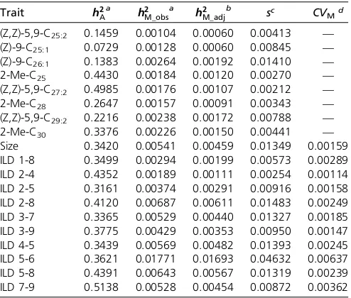
Table 1 Median additive and mutational heritability, the selection coefficient, and the coefficient of mutational variance for each trait (defined in Figure 1)
Trait h2
Aa h2M_obs a h2
M_adj
b sc CV
Md
(Z,Z)-5,9-C25:2 0.1459 0.00104 0.00060 0.00413 —
(Z)-9-C25:1 0.0729 0.00128 0.00060 0.00845 —
(Z)-9-C26:1 0.1383 0.00264 0.00192 0.01410 —
2-Me-C25 0.4430 0.00184 0.00120 0.00270 —
(Z,Z)-5,9-C27:2 0.4985 0.00176 0.00107 0.00212 —
2-Me-C28 0.2647 0.00157 0.00091 0.00343 —
(Z,Z)-5,9-C29:2 0.2216 0.00238 0.00172 0.00788 —
2-Me-C30 0.3376 0.00226 0.00150 0.00441 —
Size 0.3420 0.00541 0.00459 0.01349 0.00159
ILD 1-8 0.3499 0.00294 0.00199 0.00573 0.00289
ILD 2-4 0.4352 0.00189 0.00111 0.00254 0.00114
ILD 2-5 0.3161 0.00374 0.00291 0.00916 0.00158
ILD 2-8 0.4120 0.00687 0.00611 0.01483 0.00249
ILD 3-7 0.3365 0.00529 0.00440 0.01327 0.00185
ILD 3-9 0.3775 0.00429 0.00353 0.00950 0.00147
ILD 4-5 0.3439 0.00569 0.00482 0.01393 0.00245
ILD 5-6 0.3621 0.01771 0.01693 0.04632 0.00637
ILD 5-8 0.4391 0.00643 0.00567 0.01319 0.00239
ILD 7-9 0.5138 0.00528 0.00454 0.00872 0.00362
aMedian heritability (h2
A¼VA=VP;h2M¼VM=VP) estimated by applying the relevant
equation to each of the 1000 posterior estimates and then determining the me-dian of those values.
bMedianh2
M_adj¼medianh2M_observed2medianh2M_null.
cs= (medianV
M_obs2medianVM_null)/VA, where estimates ofVMcan be found in Table S2.
dCV
M=
ffiffiffiffiffiffiffiffiffiffiffiffiffiffiffiffiffiffiffiffiffiffiffiffiffiffiffiffiffiffiffiffiffiffiffiffiffiffiffiffiffiffiffiffiffiffiffiffiffiffiffiffiffiffiffiffiffiffiffiffiffiffiffiffiffiffiffiffiffiffiffiffiffiffiffi median VM_observed2medianVM_null
p
=X, whereXis the trait mean.CVM
is the same for both) (Table S2), the posterior samples are not paired. Therefore, we cannot apply the bias correction to the 1000 posterior samples but rather apply it to the summary statistic of that distribution, the median. Thus, we deter-mined the medianh2
Mfrom each distribution and from these medians calculated h2
M_adj¼h2M_observed2h2M_null (Table 1). We similarly corrected estimates ofVMscaled byVA(s) or trait mean CVM by first correcting the median estimate of VM (VM_adj¼median VM_observed2median VM_null) and then di-viding by median VA(s) or taking the square root and then dividing by the median trait meanCVM(Table 1). In the next section, we compare these adjusted estimates of mutational variance scaled by the total phenotypic variance, additive genetic variance, or the trait mean with published estimates.
Comparison of magnitudes of mutational variance
We compared our adjusted estimates of mutation with those reported for a range of morphological and life-history traits in other plant and animal taxa (Figure 4). Wing traits closely matched the observed median mutational heritability for morphological traits in other taxa, while CHCs were more similar in median heritability to life-history traits (Figure 4A). To our knowledge, we present thefirst estimate of mu-tational variation in CHCs or similar pheromone traits. Mu-tational variation in wing shape and size has been estimated previously from MA experiments inD. melanogaster(Santiago
et al. 1992; Houleet al.1996; Houle and Fierst 2013). The averageh2
MforD. melanogasterwing dimensions [in Table 1 of Houleet al.(1996)] was 0.00202 (CVM= 0.00136) compared with the slightly higher estimates in this study for D. serrata
wing centroid size of 0.00459 (0.00159) and median estimate of the 10 wing-shape traits of 0.00447 (0.00239) (Table 1). Houle and Fierst (2013) reported mutational heritability of
wing shape from estimates in both heterozygote (0.001) and homozygote (0.0024) form, both again slightly lower than our estimates.
When mutational variance is scaled by the standing genetic variance, one can calculate the average selection against a mutant heterozygote (s=VM/VA) (Barton 1990). Following the pattern for mutational heritability, medianswas typically higher for wing traits (0.0132) than for CHCs (0.0043) (Ta-ble 1 and Figure 4B). For both types of traits, the medians
was comparable to that reported previously for morphologi-cal traits and slightly below that reported for life-history traits (Figure 4B). Notably, there was a single wing trait (distance between landmarks 5 and 6) (Figure 1B) with s markedly higher than for other traits (Table 1). This was the only trait with a median selection coefficient above 0.021, which rep-resents the median level of selection against viability muta-tions (Houleet al.1996).
Tests of mutation-selection balance theory
With estimates of standing genetic and mutational variance from the same outbred population, we can begin to make direct quantitative assessments of the theoretical models of mutation-selection balance that attempt to explain the levels ofVAmaintained in the presence of stabilizing selection and mutation. For our traits, a positive relationship exists between the magnitudes ofVAand ofVM(Figure 5), and we now de-termine whether this relationship is consistent with drift alone or direct stabilizing selection on individual traits. The trait ILD 5-6, with the outlying estimate ofh2
M, has not been included in the following analyses because it would have had a highly disproportionate influence on the model-fitting ap-proach employed; we note, however, that the pattern for this trait was consistent with the predicted pattern under the house-of-cards model generated from the other 18 traits.
Figure 2 Distribution of posterior estimates for additive genetic and mutational variance (both multiplied by 1000) in the CHC (Z,Z)-5,9-C29:2.
As afirst step, the equilibrium genetic variance under a neutral model is given byVA= 2NeVM(Lynch and Hill 1986). For our experiment, where Ne = 958 and the median ad-justedVM= 4.5231026(Table S2), this equation predicts an additive genetic variance of 8.65 31023, twenty times greater than the observed medianVAof these traits (0.3973 1023) (Table S2). This neutral expectation is plotted in Fig-ure 5 on the heritability scale and clearly demonstrates that assuming no selection acting against mutations affecting these traits results in substantial overestimation of the stand-ing genetic variance given the observed mutational variance. The failure of this model is not surprising given the evidence for selection acting on both wing and CHC traits in this and relatedDrosophilaspecies (Hineet al.2011; McGuiganet al.
2011; McGuigan and Blows 2013).
Next, we considered two competing models of drift-mutation-selection balance for a single trait under direct stabilizing selection. First, assuming that the variance in heterozygous effects of mutations at each locus follows a Gaussian distri-bution, the Gaussian allelic approximation for mutation-selection equilibrium is given by Lynch and Lande (1993) as
VA¼
ffiffiffiffiffiffiffiffiffiffiffiffiffiffiffiffiffiffiffiffiffiffiffiffiffiffiffiffiffiffiffiffiffiffiffiffiffiffiffi
ℓVs
2Ne !2
þ2ℓVsVM v
u u
t 2ℓVs
2Ne
(5)
whereℓis the number of loci that contribute to the trait,Vsis the strength of stabilizing selection on the trait (scaled byVP), and h2
A and h2Mare substituted for VA andVMto place the prediction on the heritability scale. Although most theoretical work assumesVs$20, empirical estimates of this parameter are lower (median = 5) (Kingsolveret al.2001, 2012; Johnson
and Barton 2005), so wefixedVs= 5 tofit Equation (5) to the data. Maximum-likelihood optimization was conducted using the NLMIXED procedure in SAS (v. 9.3) (SAS Institute 2011). Figure 5 shows the fit to the data of this model (22LL =
223.9, AIC =219.9) when the maximum-likelihood esti-mate of ℓ= 4.2 is used. It is important to note that this model-fitting approach is not employed to give biologically interpretable estimates of the parameterℓbecause it is com-pletely confounded with Vs, which we fix atVs = 5 tofit model (5).
Using an alternative set of assumptions known as the
house-of-cards mutational scheme, the distribution of mutational effects at each locus is assumed to be highly leptokurtic, with most VM contributed by rare alleles of larger effect (Johnson and Barton 2005). The stochastic house-of-cards approximation for a single trait under direct stabilizing selection is given by (Bürger 2000, equation 2.15)
VA¼
2VM
VM
2þ 1
U Vs
þN21 e
(6)
whereUis genomic per-trait mutation rate, which is thought to be on the order ofU= 0.1 (Lynch and Walsh 1998). Again
fixingVs= 5 and substitutingh2Aandh2MforVAandVM, wefit this model to the data (22LL =228.6, AIC =224.6), and Figure 5 shows the result when the maximum-likelihood es-timate ofU= 0.061 is used. As withℓ, this analysis cannot provide a biologically interpretable estimate ofUbecause it is confounded withVs, which wefix [see model (6)]. Compar-ison of the Akaike information criterion (AIC) suggests that the house-of-cards model is a betterfit to the observed data than the Gaussian allelic approximation. However, as we dis-cuss later, both models tend to overestimate the predicted genetic variance when more biologically plausible parameter values are used.
Discussion
The generation of new mutational variance in natural pop-ulations has widespread evolutionary implications, and a key goal is to understand the consequences of mutation in pop-ulations evolving in the vicinity of their adaptive optimum under natural levels of recombination and outcrossing (Lynch
et al. 1999). The mutational numerator relationship matrix developed by Wray (1990), when used within an animal model, has the potential to change our approach to this
dif-ficult task. This approach allows the estimation of mutational parameters from a wide array of taxa and traits in the same way that the widespread adoption of the animal model itself expanded the study of genetic variance beyond the labora-tory or captive bred populations.
Mutational variance in an outbred population
The estimated mutational heritability in wing shape and CHCs for D. serrata males was very similar in magnitude to that reported from inbred-line experimental designs applied to
D. melanogaster. Lynchet al.(1999) reported the range of pub-lished estimates ofh2
Mto be 0.0005–0.005 forD. melanogaster, matching the range found here forD. serrataof 0.0006–0.006 with one exception. The similarity in the magnitude of h2
M between estimates derived from inbred and outbred experi-mental populations is surprising because there are two rea-sons that could causeh2
Mmeasured in an MCN experimental design to be downwardly biased in comparison to an inbred population. First, in MCN experimental designs, the high (relative to inbred lines) within-family variance provides the opportunity for selection to act (Lynch et al. 1999; Moorad and Hall 2009), under our experimental design, via competition among full siblings within each family vial. Selection against new deleterious mutations then could re-sult in an underestimation of the mutational variance. It is worth noting that selection likely operates on inbred MA di-vergence lines to an underappreciated extent (Keightleyet al.
1993; Lynch et al.1999; McGuigan and Blows 2013), sug-gesting that the comparison of estimates from the different methods is not simply one between the presence and absence of selection.
Second, in the MCN design, mutational effects are char-acterized in a heterozygous genetic background in contrast to studies of inbred MA lines, where effects are typically de-termined in homozygous form. If many mutations are re-cessive, heterozygous effects of mutations on the phenotype will be smaller than homozygous effects, consequently re-ducing the level of mutational heritability detected under the MCN design. This question of dominance has been explicitly addressed in inbred-line MA studies by crossing among MA lines to estimate mutational effects in heterozygotes. For instance, Houle and Fierst (2013) reported two to three times higher mutational heritability of wing shape when estimated from crosses within vs. among MA lines. Although crosses among MA lines assess dominance effects of mutations, the genetic background within which these mutations are assessed
is still relatively genetically depauperate. There are few esti-mates of heterozygous mutational heritability in outbred populations (see Shabalina et al. 1997; Roles and Conner 2008). The only other estimate that we are aware of to come from application of Wray’s method (Wray 1990) in an out-bred population ish2
M= 0.006 for litter size in a domesticated sheep population (Casellaset al. 2010). That estimate is at the upper end of reported estimates of mutational heritability in life-history traits (Houleet al.1996) and at the upper range of our estimates here for morphological traits. Overall, it ap-pears that neither source of potential downward bias (within family selection or heterozygous effects) has had a discern-ible impact onh2
Mestimated in our outbred population. The magnitude of the mutational variance estimated from inbred populations therefore may be broadly representative of the variance generated by the effects of heterozygous mutations, although further studies in other taxa and traits are needed to confirm this.
It follows that estimates of selection coefficients derived from inbred lines also may reflect the magnitude of selection against heterozygous mutations, of particular interest in models of mutation-selection balance. To the best of our knowledge, our estimates of selection coefficients (Table 1) represent thefirst in which both the numerator and the de-nominator have been estimated in the same outbred popula-tion; previous estimates of selection coefficients of new mutations were the product of combining estimates of VM andVA(orVG) from different experiments on distinct popu-lations (e.g., outbred forVAand inbred forVM) (Houleet al. 1996). The ratioVM/VAestimated from the same data in an outbred population reflects the heterozygous effects of new mutations in an outbred genetic background, which closely resembles how mutations would affect the phenotype when theyfirst arise in a natural population. Our estimates have a median of 0.008, comparable to the median estimate for mor-phologic traits reported for a range of taxa (Houleet al.1996),
Figure 4 Mutational heritability and selection coefficients of traits in this study (“CHC”and“Wing”
suggesting an average persistence time of mutations affecting such traits of about 125 generations.
Limitations of the experimental design
Despite several lines of evidence that suggested we success-fully captured the effects of mutation in an outbred popula-tion, we were unable to provide evidence for statistically significant mutational variance in any single trait. Similar problems have been encountered when applying the animal model to estimate additive genetic variation in wild popula-tions; when estimating quantitative genetic parameters under natural conditions, data will be more variable and larger sample sizes are required to provide sufficient statistical power (Kruuk 2004). In our experiment, greater variability was introduced not by the environment (as in wild popula-tions) but because we were focused on mutational variance while allowing standing genetic variation to persist in our experimental population, a key feature that allowed us to estimate mutational effects in the heterozygous state.
In general, and ignoring biases introduced by maternal and environmental effects (Clémentet al.2001; Kruuk and Hadfield 2007), in an animal model analysis of genetic var-iation, statistical power is determined by the size of the base population, accuracy is determined by the number of pedi-gree links between levels of thefixed effects (i.e., generations in our case) (Kennedy and Trus 1993; Hanocq et al.1996; Clémentet al.2001; Quinnet al.2006), and precision is de-termined by the number of phenotypes per family (Quinn
et al.2006). All these properties of the experimental design are captured by the T-matrix and hence should apply to both additive genetic [Equation (2)] and mutational [Equation (4)] effects. For our particular experimental design, consist-ing of 120 base-population males with a pedigree maintained
for a further 21 generations and one individual measured per family, we favored accuracy, likely at the expense of power and precision. We expect that increasing the number of indi-viduals sampled in the base population and measuring the phenotypes of multiple individuals from each family would result in greater power to detect effects and more precise estimates of mutational variance.
Mutation-selection balance in an outbred population
The processes maintaining genetic variation in natural pop-ulations remain one of the unresolved questions in evolution (Johnson and Barton 2005). Genetic variation might be main-tained by balancing selection, favoring alternate alleles or phe-notypes, or through the balance between the input of new mutations and their elimination via selection. Mutation is not an explicit parameter of balancing selection models, although it is the ultimate source of the genetic variance maintained under this mode of selection. Here we explored the implications of the observed magnitudes of standing and mutational variance for models of mutation-selection balance. Mutation-selection balance models of the maintenance of genetic variation have struggled to reconcile the general observations of strong stabi-lizing selection, high heritability, and high mutation in natural populations (Johnson and Barton 2005). Consistent with this view, both the Gaussian and house-of-cards models tended to overestimate the standing level ofVAin this population when compared to the data. Notably, we assumed strong selection (Vs= 5) compared toVs$20 that is used in most theoretical treatments (Johnson and Barton 2005) of mutation-selection balance. Weakening the strength of selection increases the equilibrium VApredicted by these models, further worsening theirfit to the observed data. Similarly, forcing the other two parameters that were free to vary, ℓandU, to possibly more realistic values, say,ℓ.10 orU= 0.1 (Lynch and Walsh 1998), also increases the equilibrium level ofVA.
Johnson and Barton (2005) identified three different clas-ses of mutation-selection balance models: direct stabilizing selection on individual traits, direct selection on multiple traits, and pure pleiotropy models (see also Zhang and Hill 2005). Having shown that direct selection on single traits is unlikely to adequately explain the estimated levels of addi-tive and mutational genetic variance in this outbred popula-tion of D. serrata, we highlight two points concerning the other two classes of mutation-selection balance models. First, we can exclude the pure pleiotropy model as a good fit to these data based on our current estimates. Under the pure pleiotropy class of model, observed mutational heritability on the order of 0.001 implies that standardized stabilizing selec-tion gradients on traits must be20.001 (Vs= 500) or weaker to maintain any level of heritability (Johnson and Barton 2005, equation A25). While this strength of stabilizing selec-tion has been observed on the genetic variance of some indi-vidual CHC traits, it varies considerably among traits and has been reported to be up to 100 times stronger on one CHC expressed in males of our study species (Delcourtet al.2012). A pure pleiotropy model of mutation-selection balance is
therefore unable to explain the levels of heritability in this outbred population given the strength of stabilizing selection that has been observed on some of these traits.
Second, it is well known that the morphological traits analyzed here are not genetically independent of one another (Blows et al.2004; Mezey and Houle 2005; McGuigan and Blows 2007; Houle and Fierst 2013; Hineet al.2014), and such pleiotropy will tend to reduce the level of heritability that can be maintained under mutation-selection balance (Bürger 2000, p. 298). This suggests that a multivariate assessment of mutation-selection balance might be infor-mative given that single-trait models generally overestimated the predicted heritability. An assessment of the multivariate extension of the direct selection model requires estimation of the additive and mutational variance-covariance matrices (Lande 1980), which we are currently pursuing for these traits. How genetic variation is maintained in the presence of selection remains one of the fundamental unresolved issues in evolutionary biology and a key question given that mutation and stabilizing selection are ubiquitous evolutionary forces (Turelli 1984; Johnson and Barton 2005; Walsh and Blows 2009). Mutation-selection balance is one of the two leading explanations (along with balancing selection) for the levels of standing variance in natural populations (Barton 1990; Johnson and Barton 2005; Zhang and Hill 2005), but the data available on key mutation parameters are sparse and of low quality (Houle et al. 1996). Wray’s insight (Wray 1990) has provided us with a way of estimating key muta-tional parameters in an outbred population. By combining these estimates of mutation genetic variance with estimates of standing genetic variance derived from the same popula-tion and statistical model, more detailed and internally con-sistent investigations of mutation-selection balance in outbred populations become feasible.
Acknowledgments
We thank D. Petfield, A. Denton, and M. E. Vidgen for main-taining this experiment over 18 months; N. Wray, H. S. Lee, and J. Hadfield for discussions on the implementation of the M-matrix animal model; and D. Houle and an anonymous reviewer for comments on a previous version of the manu-script. This research was funded by the Australian Research Council.
Literature Cited
Aguirre, J. D., M. W. Blows, and D. J. Marshall, 2014 The genetic covariance between life cycle stages separated by metamorpho-sis. Proc. Biol. Sci. 281: 20141091.
Aitchison, J., 1986 The Statistical Analysis of Composition Data. Chapman & Hall, London.
Barton, N. H., 1990 Pleiotropic models of quantitative variation. Genetics 124: 773–782.
Blows, M. W., and R. A. Allan, 1998 Levels of mate recognition within and between two Drosophilaspecies and their hybrids. Am. Nat. 152: 826–837.
Blows, M. W., S. F. Chenoweth, and E. Hine, 2004 Orientation of the genetic variance-covariance matrix and the fitness surface for multiple male sexually selected traits. Am. Nat. 163: E329– E340.
Bürger, R., 2000 The Mathematical Theory of Selection, Recombi-nation,and Mutation. Wiley, Chichester, UK.
Casellas, J., and J. R. Medrano, 2008 Within-generation mutation variance for litter size in inbred mice. Genetics 179: 2147–2155. Casellas, J., G. Caja, and J. Piedrafita, 2010 Accounting for addi-tive genetic mutations on litter size in Ripollesa sheep. J. Anim. Sci. 88: 1248–1255.
Chenoweth, S. F., H. D. Rundle, and M. W. Blows, 2010 The
contribution of selection and genetic constraints to phenotypic divergence. Am. Nat. 175: 186–196.
Clément, V., B. Bibé, É. Verrier, J. M. Elsen, E. Manfredi et al., 2001 Simulation analysis to test the influence of model ade-quacy and data structure on the estimation of genetic parame-ters for traits with direct and maternal effects. Genet. Sel. Evol. 33: 369–396.
Crow, J. F., and M. Kimura, 1970 An Introduction to Population Genetics Theory. Harper & Row, New York.
Delcourt, M., M. W. Blows, J. D. Aguirre, and H. D. Rundle, 2012 Evolutionary optimum for male sexual traits character-ized using the multivariate Robertson-Price Identity. Proc. Natl. Acad. Sci. USA 109: 10414–10419.
Denver, D. R., K. Morris, J. T. Streelman, S. K. Kim, M. Lynchet al., 2005 The transcriptional consequences of mutation and natu-ral selection inCaenorhabditis elegans. Nat. Genet. 37: 544–548. Frentiu, F. D., and S. F. Chenoweth, 2008 Polyandry and pater-nity skew in natural and experimental populations ofDrosophila serrata. Mol. Ecol. 17: 1589–1596.
Gelman, A., 2006 Prior distributions for variance parameters in hierarchical models. Bayesian Anal. 1: 515–533.
Gelman, A., and D. B. Rubin, 1992 Inference from iterative sim-ulation using multiple sequences. Stat. Sci. 7: 457–472. Gosden, T. P., K. L. Shastri, P. Innocenti, and S. F. Chenoweth,
2012 The B-matrix harbors significant and sex-specific con-straints on the evolution of multicharacter sexual dimporphism. Evolution 66: 2106–2116.
Haag-Liautard, C., M. Dorris, X. Maside, S. Macaskill, D. L. Halligan et al., 2007 Direct estimation of per nucleotide and genomic deleterious mutation rates inDrosophila. Nature 445: 82–85. Hadfield, J. D., 2010 MCMC methods for multi-response
general-ized linear mixed models: the MCMCglmm R package. J. Stat. Softw. 33: 1–22.
Hadfield, J. D., 2014 MCMCglmm course notes; available at:
cran.r-project.org/web/packages/MCMCglmm/vignettes/Cour-seNotes.pdf.
Hadfield, J. D., A. J. Wilson, D. Garant, B. C. Sheldon, and L. E. B.
Kruuk, 2010 The misuse of BLUP in ecology and evolution.
Am. Nat. 175: 116–125.
Halligan, D. L., and P. D. Keightley, 2009 Spontaneous mutation accumulation studies in evolutionary genetics. Annu. Rev. Ecol. Evol. Syst. 40: 151–172.
Hanocq, E., D. Boichard, and J. L. Foulley, 1996 A simulation study of the effect of connectedness on genetic trend. Genet. Sel. Evol. 28: 67–82.
Hansen, T. F., C. Pelabon, and D. Houle, 2011 Heritability is not evolvability. Evol. Biol. 38: 258–277.
Henderson, C. R., 1976 A simple method for computing the in-verse of a numerator relationship matrix used in prediction of breeding values. Biometrics 32: 69–83.
Hine, E., K. McGuigan, and M. W. Blows, 2011 Natural selection stops the evolution of male attractiveness. Proc. Natl. Acad. Sci. USA 108: 3659–3664.
Hine, E., K. McGuigan, and M. W. Blows, 2014 Evolutionary con-straints in high-dimensional trait sets. Am. Nat. 184: 119–131. Houle, D., and J. Fierst, 2013 Properties of spontaneous muta-tional variance and covariance for wing size and shape in Dro-sophila melanogaster. Evolution 67: 1116–1130.
Houle, D., B. Morikawa, and M. Lynch, 1996 Comparing
muta-tional variabilities. Genetics 143: 1467–1483.
Houle, D., C. Pelabon, G. P. Wagner, and T. F. Hansen,
2011 Measurement and meaning in biology. Q. Rev. Biol.
86: 3–34.
Johnson, T., and N. Barton, 2005 Theoretical models of selection and mutation on quantitative traits. Philos. Trans. R. Soc. Lond. B Biol. Sci. 360: 1411–1425.
Keightley, P. D., and W. G. Hill, 1992 Quantitative genetic varia-tion in body size of mice from new mutavaria-tions. Genetics 131: 693–700.
Keightley, P. D., T. F. C. Mackay, and A. Caballero,
1993 Accounting for bias in estimates of the rate of polygenic mutation. Proc. Biol. Sci. 253: 291–296.
Keightley, P. D., A. Caballero, and A. Garcia-Dorado,
1998 Population genetics: surviving under mutation pressure. Curr. Biol. 8: R235–R237.
Keightley, P. D., U. Trivedi, M. Thomson, F. Oliver, S. Kumaret al., 2009 Analysis of the genome sequences of three Drosophila melanogasterspontaneous mutation accumulation lines. Genome Res. 19: 1195–1201.
Keightley, P. D., R. W. Ness, D. L. Halligan, and P. R. Haddrill, 2014 Estimation of the spontaneous mutation rate per nucle-otide site in aDrosophila melanogasterfull-sib family. Genetics 196: 313–320.
Keightley, P. D., A. Pinharanda, R. W. Ness, F. Simpson, K. K.
Dasmahapatra et al., 2015 Estimation of the spontaneous
mutation rate in Heliconius melpomene. Mol. Biol. Evol. 32: 239–243.
Kennedy, B. W., and D. Trus, 1993 Considerations on genetic
connectedness between management units under an animal model. J. Anim. Sci. 71: 2341–2352.
Kingsolver, J. G., H. E. Hoekstra, J. M. Hoekstra, D. Berrigan, S. N. Vignieri et al., 2001 The strength of phenotypic se-lection in natural populations. Am. Nat. 157: 245–261. Kingsolver, J. G., S. E. Diamond, A. M. Siepielski, and S. M. Carlson,
2012 Synthetic analyses of phenotypic selection in natural populations: lessons, limitations and future directions. Evol. Ecol. 26: 1101–1118.
Kondrashov, A. S., and M. Turelli, 1992 Deleterious mutations, apparent stabilizing selection and the maintenance of quantita-tive variation. Genetics 132: 603–618.
Kruuk, L. E. B., 2004 Estimating genetic parameters in natural populations using the “animal model.” Philos. Trans. R. Soc. Lond. B Biol. Sci. 359: 873–890.
Kruuk, L. E. B., and J. D. Hadfield, 2007 How to separate genetic and environmental causes of similarity between relatives. J. Evol. Biol. 20: 1890–1903.
Lande, R., 1975 Maintenance of genetic variability by mutation in polygenic character with linked loci. Genet. Res. 26: 221–235.
Lande, R., 1980 The genetic covariances between characters
maintained by pleiotropic mutations. Genetics 94: 203–215. Lande, R., 1995 Mutation and conservation. Conserv. Biol. 9:
782–791.
Lynch, M., and W. G. Hill, 1986 Phentoypic evolution by neutral mutation. Evolution 40: 915–935.
Lynch, M., and R. Lande, 1993 Evolution and extinction in
response to environmental change, pp. 234–250 in Biotic Inter-actions and Global Climate Change, edited by P. M. Kareiva,
J. G. Kingsolver, and R. B. Huey. Sinauer Associates, Sunderland, MA.
Lynch, M., and B. Walsh, 1998 Genetics and Analysis of Quantita-tive Traits. Sinauer Associates, Sunderland, MA.
Lynch, M., J. Blanchard, D. Houle, T. Kibota, S. Schultz et al., 1999 Spontaneous deleterious mutation. Evolution 53: 645– 663.
Mack, P. D., V. K. Lester, and D. E. L. Promislow, 2001 Age-specific effects of novel mutations inDrosophila melanogaster. II. Fecun-dity and male mating ability. Genetica 110: 31–41.
McGuigan, K., and M. W. Blows, 2007 The phenotypic and genet-ic covariance structure of Drosophilid wings. Evolution 61: 902– 911.
McGuigan, K., and M. W. Blows, 2013 Joint allelic effects on
fitness and metric traits. Evolution 67: 1131–1142.
McGuigan, K., L. Rowe, and M. W. Blows, 2011 Pleiotropy, appar-ent stabilizing selection and uncoveringfitness optima. Trends Ecol. Evol. 26: 22–29.
McGuigan, K., J. M. Collet, S. L. Allen, S. F. Chenoweth, and M. W. Blows, 2014 Pleiotropic mutations are subject to strong stabi-lizing selection. Genetics 197: 1051–1062.
Mezey, J. G., and D. Houle, 2005 The dimensionality of genetic variation for wing shape inDrosophila melanogaster. Evolution 59: 1027–1038.
Moorad, J. A., and D. W. Hall, 2009 Mutation accumulation, soft selection and the middle-class neighborhood. Genetics 182: 1387–1389.
Mousseau, T. A., and D. A. Roff, 1987 Natural selection and the heritability offitness components. Heredity 59: 181–197. Partridge, L., A. Hoffmann, and J. S. Jones, 1987 Male size and
mating success inDrosophila melanogasterandD. pseudoobscura underfield conditions. Anim. Behav. 35: 468–476.
Quinn, J. L., A. Charmantier, D. Garant, and B. C. Sheldon, 2006 Data depth, data completeness, and their influence on quantitative genetic estimation in two contrasting bird popula-tions. J. Evol. Biol. 19: 994–1002.
Robertson, F. W., and E. Reeve, 1952 Studies in quantitative in-heritance. I. The effects of selection of wing and thorax length in Drosophila melanogaster. J. Genet. 50: 414–448.
Roff, D. A., and T. A. Mousseau, 1987 Quantitative genetics and
fitness: lessons fromDrosophila. Heredity 58: 103–118. Rohlf, F. J., 1999 Shape statistics: procrustes superimpositions
and tangent spaces. J. Classif. 16: 197–223.
Roles, A. J., and J. K. Conner, 2008 Fitness effects of mutation accumulation in a natural outbred population of wild radish (Raphanus raphanistrum): comparison offield and greenhouse environments. Evolution 62: 1066–1075.
Rundle, H. D., S. F. Chenoweth, P. Doughty, and M. W. Blows, 2005 Divergent selection and the evolution of signal traits and mating preferences. PLoS Biol. 3: 1988–1995.
Santiago, E., J. Albornoz, A. Dominguez, M. A. Toro, and C. Lopez-Fanjul, 1992 The distribution of spontaneous mutations on quantitative traits andfitness inDrosophila melanogaster. Genet-ics 132: 771–781.
SAS Institute, 2011 SAS 9.3. Cary, NC.
Schultz, S. T., and M. Lynch, 1997 Mutation and extinction: the role of variable mutational effects, synergistic epistasis, benefi -cial mutations, and degree of outcrossing. Evolution 51: 1363– 1371.
Shabalina, S. A., L. Y. Yampolsky, and A. S. Kondrashov, 1997 Rapid decline offitness in panmictic populations of Dro-sophila melanogaster maintained under relaxed natural selec-tion. Proc. Natl. Acad. Sci. USA 94: 13034–13039.
Turelli, M., 1984 Heritable genetic variation via mutation selec-tion balance: Lerch’s zeta meets the abdominal bristle. Theor. Popul. Biol. 25: 138–193.
Walsh, B., and M. W. Blows, 2009 Abundant genetic variation
+ strong selection = multivariate genetic constraints: a geometric view of adaptation. Annu. Rev. Ecol. Evol. Syst. 40: 41–59.
Whitlock, M. C., 2000 Fixation of new alleles and the extinction of small populations: drift load, beneficial alleles, and sexual selection. Evolution 54: 1855–1861.
Wilson, A. J., D. Reale, M. N. Clements, M. M. Morrissey, E. Postma et al., 2010 An ecologist’s guide to the animal model. J. Anim. Ecol. 79: 13–26.
Wray, N. R., 1990 Accounting for mutation effects in the additive genetic variance covariance matrix and its inverse. Biometrics 46: 177–186.
Yampolsky, L. Y., L. E. Pearse, and D. E. L. Promislow, 2001 Age-specific effects of novel mutations inDrosophila melanogaster. I. Mortality. Genetica 110: 11–29.
Zhang, X. S., and W. G. Hill, 2002 Joint effects of pleiotropic selection and stabilizing selection on the maintenance of quantitative genetic variation at mutation-selection balance. Genetics 162: 459–471. Zhang, X. S., and W. G. Hill, 2005 Genetic variability under
mu-tation selection balance. Trends Ecol. Evol. 20: 468–470.
GENETICS
Supporting Information
www.genetics.org/lookup/suppl/doi:10.1534/genetics.115.178632/-/DC1
Simultaneous Estimation of Additive and
Mutational Genetic Variance in an Outbred
Population of
Drosophila serrata
Katrina McGuigan, J. David Aguirre, and Mark W. Blows
!
1!
Table S1. Correlation between
estimates!of!V
A!and!V
M!
from the observed data, and the null
model in which the pedigree was randomized. Traits are defined in Figure 1.
Trait!
Observed!Data!
Null!Model!
Z,Z–5,9–C
25:2!
A0.288!
A0.001!
Z–9–C
25:1!
A0.238!
0.026!
Z–9–C
26:1!
A0.590!
A0.035!
2–Me–C
25!
A0.612!
A0.028!
Z,Z–5,9–C
27:2!
A0.487!
A0.045!
2–Me–C
28!
A0.483!
0.011!
Z,Z–5,9–C
29:2!
A0.661!
A0.059!
2–Me–C
30!
A0.652!
A0.043!
Centroid!Size!
A0.868!
A0.040!
ILD!1–8!
A0.742!
0.011!
ILD!2–4!
A0.500!
A0.062!
ILD!2–5!
A0.741!
A0.029!
ILD!2–8!
A0.908!
A0.029!
ILD!3–7!
A0.864!
A0.046!
ILD!3–9!
A0.855!
A0.037!
ILD!4–5!
A0.871!
0.008!
ILD!5–6!
A0.943!
A0.100!
ILD!5–8!
A0.905!
A0.090!
Table&S2.
!Median!estimates!(and!95%!confidence!intervals)!(x1000)!of!variance!components!for!additive!genetic!(V
A),!mutational!(V
M)!and!
total!phenotypic!(V
P)!variance!from!the!null!model!and!the!observed!data.!Note,!the!phenotypic!data!was!identical!between!the!two!datasets,!
but!pedigree!information!was!randomised!in!the!null!data.!As!V
P!is!therefore!the!same!in!the!two!datasets,!only!the!median!of!the!1000!
iterations!of!the!observed!data!is!shown.!
Trait! VA!Null! VA!Observed! VM!Null! VM!Observed! VP!
Z,Z–5,9–C25:2! 0.2555! 0.7754*! 0.00232! 0.00553! 5.3260!
! (0.1266!R!0.5050)! (0.5052!–!1.0846)! (0.00000!R!0.02410)! (0.00001!R!0.06242)! (5.0993!–!5.5363)!
Z–9–C25:1! 0.0007278! 1.1119! 0.01035! 0.01974! 15.3449!
! (0.3591!–!1.4126)! (0.5841!–!1.9374)! (0.00001!R!0.11958)! (0.00004!R!0.22260)! (14.6847!–!15.9783)!
Z–9–C26:1! 0.6397! 1.8605! 0.00974! 0.03597! 13.4905!
! (0.3322!–!1.2223)! (0.!9100!R!0.0026449)! (0.00002!R!0.10169)! (0.00007!R!0.42070)! (12.7015!–!14.0730)!
2–Me–C25! 0.9402! 8.7760*! 0.01277! 0.03648! 19.8280!
! (0.4639!R!0.0018208)! (6.6495!R!10.2711)! (0.00002!R!0.13630)! (0.00007!R!0.67487)! (18.6527!–!20.8207)!
Z,Z–5,9–C27:2! 0.6328! 6.3428*! 0.00898! 0.02244! 12.7681!
! (0.3187!–!1.2930)! (5.3029!R!0.0073773)! (0.00002!R!0.08130)! (0.00005!R!0.31425)! (12.0653!–!13.3346)!
2–Me–C28! 0.6967! 3.7755*! 0.00934! 0.02231! 14.1896!
Z,Z–5,9–C29:2! 0.8973! 4.1439*! 0.01226! 0.04492! 18.7076!
! (0.4322!–!1.6235)! (2.1588!–!5.4126)! (0.00003!R!0.13952)! (0.00008!R!0.68827)! (17.3659!–!19.5281)! 2–Me–C30! 0.9045! 6.1084*! 0.01380! 0.04073! 18.0120!
! (0.4500!–!1.7195)! (4.2395!–!7.3787)! (0.00002!R!0.17019)! (0.00010!R!0.61536)! (16.8318!–!18.7980)! Centroid!Size! 0.0776! 0.5113*! 0.00124! 0.00814! 1.4891!
! (0.0385!R!0.1536)! (0.1836!R!0.6582)! (0.00000!R!0.01450)! (0.00001!R!0.12860)! (1.2636!–!1.5714)! ILD!1–8! 0.0127! 0.0849*! 0.00023! 0.00072! 0.2420!
! (0.0065!R!0.0259)! (0.0506!R!0.1045)! (0.00000!R!0.00232)! (0.00000!R!0.01245)! (0.2198!R!0.2535)! ILD!2–4! 0.0178! 0.1516*! 0.00027! 0.00066! 0.3489!
! (0.0083!R!0.0341)! (0.1185!R!0.1798)! (0.00000!R!0.00313)! (0.00000!R!0.00932)! (0.3281!R!0.3649)! ILD!2–5! 0.0321! 0.1949*! 0.00051! 0.00230! 0.6137!
! (0.0153!R!0.0631)! (0.0965!R!0.2475)! (0.00000!R!0.00567)! (0.00001!R!0.03507)! (0.5532!R!0.6458)! ILD!2–8! 0.0502! 0.3970*! 0.00074! 0.00663! 0.9600!
! (0.0257!R!0.1036)! (0.1171!R!0.4934)! (0.00000!R!0.01020)! (0.0002!R!0.10964)! (0.7714!–!1.0141)! ILD!3–7! 0.0364! 0.2368*! 0.00063! 0.00377! 0.7018!
! (0.0179!R!0.0707)! (0.0863!R!0.3049)! (0.00000!R!0.00728)! (0.00000!R!0.05793)! (0.6005!R!0.7422)! ILD!3–9! 0.0492! 0.3681*! 0.00075! 0.00425! 0.9764!
ILD!4–5! 0.0333! 0.2252*! 0.00058! 0.00371! 0.6529!
! (0.0162!R!0.0664)! (0.0769!R!0.2855)! (0.00000!R!0.00659)! (0.00001!R!0.05762)! (0.5560!R!0.6877)!
ILD!5–6! 0.0137! 0.0975! 0.00022! 0.00473! 0.2670!
! (0.0068!R!0.0275)! (0.0183!R!0.1301)! (0.00000!R!0.00277)! (0.00001!R!0.03404)! (0.2118!R!0.2872)!
ILD!5–8! 0.0243! 0.2179*! 0.00038! 0.00325! 0.4940!
! (0.0118!R!0.0492)! (0.0697!R!0.2631)! (0.00000!R!0.00451)! (0.00001!R!0.05439)! (0.3947!R!0.5214)!
ILD!7–9! 0.0182! 0.1897*! 0.00028! 0.00193! 0.3677!
! (0.0089!R!0.0365)! (0.0740!R!0.2261)! (0.00000!R!0.00368)! (0.00000!R!0.04332)! (0.2881!R!0.3890)!