ABSTRACT
QUINTANILLA BERJON, VERONICA. Fuel Loads, Prescribed Fire and Fire Effects in Longleaf Ecosystems: Analysis of Fuel Consumption and Mortality. A Case Study in the Calloway Forest Preserve, NC. (Under the direction of Dr. Joseph Roise, Dr. Glenn Catts and Dr. Heather Cheshire).
Land managers involved in longleaf restoration are increasingly using fire as
management tool to restore and maintain this highly diverse and endangered fire dependent
ecosystem. However, to achieve restoration goals it is necessary to better understand the
relationships between stand conditions, fuel loadings, fire behavior, fire effects and
ecosystem responses. This information would help to plan accordingly to reach short and
long term management goals and avoid undesired fire effects (longleaf mortality).
In this case study, detailed analysis of pre, during and post burn conditions were
conducted in a mature longleaf-wiregrass stand in the Calloway Forest Preserve (NC). Before
burning a fuel loading inventory was conducted using two different fuel sampling methods,
planar intersect (PI) and biomass collection destructive sampling. Estimates from both
methods were compared for five different fuel types. Fire conditions and fire behavior were
recorded and related with fire intensities and fire effects. Fuel consumption turned out to be
higher than expected in the burn plan and an equation to predict forest floor depth removal
was developed for future prediction. Fire intensity was found highly variable and hotter than
expected. Fire severity effects analyzed in the overstory pointed to no direct association
between percentage of crown scorched and tree mortality. Longleaf seedling mortality was
found to be related with fire temperature and height; especially in seedlings between 0.3 and
© Copyright 2015 Veronica Quintanilla Berjon
Fuel Loads, Prescribed Fire and Fire Effects in Longleaf Ecosystems: Analysis of Fuel Consumption and Mortality. A Case Study in the Calloway Forest Preserve, NC
by
Veronica Quintanilla Berjon
A thesis submitted to the Graduate Faculty of North Carolina State University
in partial fulfillment of the requirements for the degree of
Master of Science
Forestry and Environmental Resources
Raleigh, North Carolina
2015
APPROVED BY:
_______________________________ Dr. Joseph Roise
DEDICATION
I dedicate this thesis to my husband and close friends, who provided me with nothing but
support and encouragement throughout this journey into the scientific word in a second
BIOGRAPHY
Veronica Quintanilla Berjon was born in a small town in Leon, Spain. She completed a
Technical Engineering Degree in Forestry at the University of Leon (Spain) and a Forest
Engineering Degree at the University of Lleida (Spain). As part of her B.S. thesis project,
Veronica made an academic exchange with the University of Chapingo (Mexico), where she
started developing her interest in wildland fire topics and focused her thesis research in the
Evaluation of Forest Fuels through Geographic Information Systems (GIS).
Throughout her career Veronica has been closely involved with numerous Non-Profit
Organizations focused in natural conservation and rural development and she loves working
in sustainable community development. She is passionate about wildland fire and before
moving to the United States to pursue her M.S. at North Carolina State University, she
worked as a firefighter in a helitack crew in the North of Spain. She is planning to keep
travelling and discovering new countries, cultures and languages while she continues
ACKNOWLEDGMENTS
I would like to express my sincerest appreciation to the members of my advisory committee
and all faculty members (at NCSU and other institutions) that have shared with me their time,
knowledge, and expert opinion. Special thanks to my major advisor, Dr. Joseph Roise, for
allowing me the opportunity to be a graduate student and conduct this research with no
creative limitations and with his endless support and enthusiasm. I express my great gratitude
towards Dr. Glenn Catts, Dr. Heather Cheshire and Robert Mickler for providing technical
guidance and priceless advice; and to Dr. Jorge Montero, Dr. Fikret Isik and Nasir Shalizi for
sharing their invaluable statistical support.
I express my great gratitude towards The Nature Conservancy and its incredible staff, who
have been an essential part in the development of this thesis; thanks for being open to discuss
current management concerns and practical research questions, support me with the study
area and provide funding for the project. Special thanks are owed to Margit Bucher and
Gretchen Coll for sharing their time and knowledge, providing their invaluable support and
helping me to develop my scientific insight and fire career. I also would like to thank Mike
Norris for being open to conduct this research and providing the study area; and Ryan
Bollinger, Tag Merchant, Katie Sauerbrey, Eden Friedrich, Natasha Whetzel, Julia Bartley,
Katelynn Jenkins, Coleman Minney and Anthony Moore for their hard work and support, I
would not have been able to complete the field work without their help.
Finally, I would like to thank to my husband, friends, and NCSU mates for their support
TABLE OF CONTENTS
LIST OF TABLES ... viii
LIST OF FIGURES ... x
CHAPTER 1: EVALUATION OF TWO FUEL SAMPLING TECHNIQUES FOR ESTIMATING SURFACE FUEL LOADING IN LONGLEAF ECOSYSTEMS... 1
ABSTRACT ... 1
INTRODUCTION ... 2
MATERIALS AND METHODS ... 4
Study Area ... 4
Calloway Forest ... 4
Burn Unit fuels general description ... 6
Analysis procedures ... 8
Fuel load definitions ... 8
Fuel load measurements ... 10
Fuel loading calculations ... 12
Data Analysis ... 18
Fuel loading distribution ... 18
Fuel loading: comparison between estimation methods ... 18
RESULTS ... 20
Fuel loading estimations and distributions ... 20
Fuel loading: comparison between estimation methods ... 26
DISCUSSION ... 30
CONCLUSIONS AND MANAGEMENT RECOMENDATIONS ... 35
CHAPTER 2: PRESCRIBED FIRE AND FIRE EFFECTS IN LONGLEAF ECOSYSTEMS: FUEL CONSUMPTION AND MORTALITY. A CASE STUDY IN THE CALLOWAY FOREST ... 38
ABSTRACT ... 38
INTRODUCTION ... 39
MATERIALS AND METHODS ... 44
Study Area ... 44
Calloway Forest: management goals ... 44
Field data collection and analysis procedures ... 46
Plot Establishment ... 46
Pre burn sampling inventory ... 46
Fuel load measurements ... 47
Understory measurements ... 48
Overstory measurements ... 48
Regeneration measurements ... 48
Fire behavior observations and data collection (ROS, weather, moisture)... 49
Fuel moisture measurements... 49
Fire Weather... 50
Maximum fire temperature ... 51
Fire rate of spread (ROS), flame height (FH) and flame length (FL) ... 52
Post burn sampling ... 54
Fire severity assessment (categorical) ... 54
Fuel load measurements ... 54
Understory measurements ... 55
Overstory measurements ... 55
Regeneration measurements ... 56
Data analysis ... 57
Fuel loads and fire effects in the forest floor: fuel consumption ... 57
Fuel loading estimations ... 57
Fuel loading distribution vs. tree density ... 57
Fuel consumption and forest floor depth removal ... 58
Fire behavior and fire effects in overstory and regeneration ... 59
Fire intensity and fire severity in the overstory ... 59
Fire effects in regeneration: seedlings mortality ... 60
Longleaf seedlings mortality, fuel consumption and maximum temperature at the unit level... 60
Analysis of longleaf seedlings mortality by height class and max. temperature at each height ... 60
RESULTS ... 63
Fuel loading estimations ... 63
Fuel loading distribution vs. Basal Area (BA)... 63
Fire weather ... 66
Fire behavior, fire intensity and maximum temperature ... 69
Fire effects: fuel consumption and mortality ... 72
Fire effects in the forest floor: fuel consumption and forest floor depth removal ... 72
Fire behavior and fire effects in overstory ... 76
Char height, maximum bole scorch height and percentage of crown scorched ... 76
Fireline intensity and fire severity in the overstory ... 79
Fire severity in the overstory and tree mortality ... 80
Fire severity in regeneration: seedlings mortality ... 81
Longleaf seedlings mortality and fuel consumption at the unit level ... 81
Longleaf seedlings/saplings mortality by height class and Temperature ... 84
DISCUSSION AND CONCLUSIONS ... 89
GENERAL BURN OBJECTIVES ACCOMPLISHMENT REVIEW... 95
MANAGEMENT RECOMMENDATIONS ... 96
REFERENCES ... 98
APPENDICES ... 111
Appendix A: Monitoring protocols for Study area ... 112
Appendix B: Pre burn fuel loads in Unit 27 at Calloway Forest Preserve. ... 114
Appendix C: Post burn fuel loads in Unit 27 at Calloway Forest Preserve ... 116
LIST OF TABLES
Table 1: Canadian and U.S soil taxonomy description correspondent to litter and duff. ... 9
Table 2: Longleaf bulk density conversion factors (tons/acre/inch) (Parresol 2005). ... 14
Table 3: Values used to transform inventory values (counts and volumes) to biomass (weight) following Brown's (1974) equations. ... 15
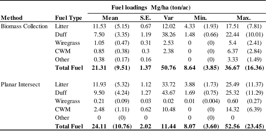
Table 4: Estimated fuel loadings for fuel type and sampling method before the burn. ... 21
Table 5: Estimated fuel loadings for fuel type and sampling method after the burn. ... 21
Table 6: Bootstrap summary statistics for all fuel types present before the burn ... 28
Table 7: Bootstrap summary statistics for all fuel types present after the burn. ... 29
Table 8: Wilcoxon-Mann-Whitney U test for significant difference between fuel types collected with two different methods ... 30
Table 9: Height class codes for seedling trees (National Park Service 2003) ... 49
Table 10: Correspondence between seedling height class, seedling height and height were maximum temperature was recorded. ... 61
Table 11: Summary table for fuel loading depths and tree density across the study unit. ... 63
Table 12: Spearman correlation coefficients between tree density and pre burn forest floor fuel loads by estimation method. ... 66
Table 13: Average rates of spread (ROS), flame heights (FH) and flame lengths (FL) observed and recorded at different locations during the burn ... 69
Table 14: Fireline intensity calculations based on Byram's equations ... 70
Table 15: Maximum temperature vertical profile recorded at the center of each plot ... 71
Table 16: Summary Statistics of fuel consumption at the Unit level by sampling method ... 73
Table 17: Parameter estimates and ANOVA table of forest floor depth removal model. ... 75
Table 18: Fire severity in the overstory. Summary statistics by tree ... 76
Table 19: Spearman correlation coefficients and probabilities between fire severity variables in the overstory. ... 79
Table 20: Summary statistics of longleaf seedlings mortality, maximum temperature and fuel consumption at the unit level. ... 82
Table 21: Longleaf regeneration mortality and mean maximum temperature at each height.85 Table 22: SAS output from GLIMMIX procedure. Model information and parameter estimates for negative binomial regression model to predict seedlings mortality ... 87
Table 24: Odds ratio estimates for seedlings mortality based on variations in height... 89
Appendix B
Table B 1: Pre burn fuel loads collected with the Biomass sample method ... 114
Table B 2: Pre burn fuel loads collected with the Planar Intersect method ... 115
Appendix C
Table C 1: Post burn fuel loads collected with the Biomass sample method. ... 116
Table C 2: Post burn fuel loads collected with the Planar Intersect method ... 117
Appendix D
LIST OF FIGURES
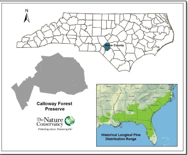
Figure 1: Calloway Forest Preserve location (Hoke County, NC). ... 6
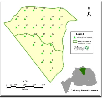
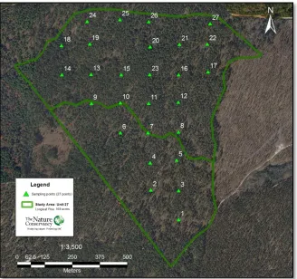
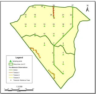
Figure 2: Study area (Burn Unit 27) with sampling points at Calloway Forest Preserve. ... 7
Figure 3: Overview of general fuel types and distributions in burn Unit 27 ... 8
Figure 4: Pre-burn fuel loads (Mg/ha) and SE by fuel type and method of estimation. ... 22
Figure 5: Post-burn fuel load (Mg/ha) and SE by fuel type and method of estimation ... 23
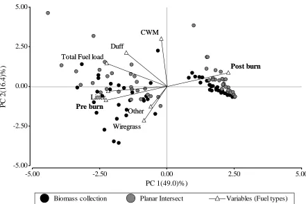
Figure 6: Principal Component Analysis (PCA) of fuel loading observations ... 24
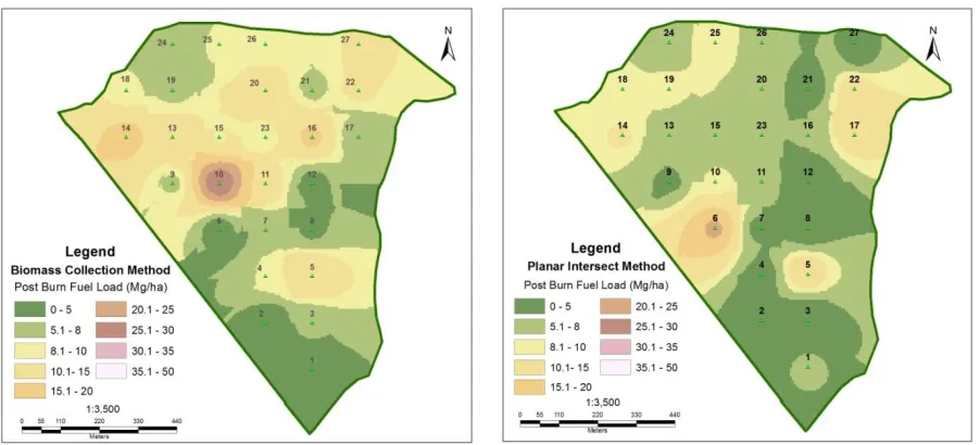
Figure 7: Maps of pre-burn fuel load estimates (Mg/ha) using biomass collection (left) and planar intersect (right) methods. ... 26
Figure 8: Maps of post-burn fuel load estimates (Mg/ha) using biomass collection (left) and planar intersect (right) methods ... 26
Figure 9: Comparison of mean total fuel load estimations and SD by collection method and fuel type before and after burning. ... 27
Figure 10: Study area limits with sampling points and vegetation cover overview. ... 46
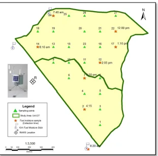
Figure 11: RAWS station and fuel moisture samples location. ... 50
Figure 12: Picture of rebar with tags painted with heat sensitive paints ... 52
Figure 13: Rate of spread (ROS), flame height (FH) and flame length (FL) observations ... 53
Figure 14: Live and dead longleaf seedlings observed in the unit 3 months after burning ... 56
Figure 15: Maps of Basal Area (BA) (m²/ha) (left) and pre-burn litter + duff depth (mm) (right) distribution across the study area. ... 64
Figure 16: Maps of pre-burn litter depth (mm) (right) and pre-burn duff depth (mm) (left) distribution across the study area. ... 64
Figure 17: Atmospheric & fuel temperatures (°C) and RH (%) recorded by RAWS ... 67
Figure 18: Temperature (°C) and wind speed (Km/h) collected with portable weather kit and RAWS during prescribed burn... 68
Figure 19: RH (%) and fine dead fuels moisture (FDM) (%) collected with portable weather kit and RAWS during prescribed burn. ... 68
Figure 20: Maximum temperature (°C) recorded at each plot ... 72
Figure 21: Fuel consumption mean estimates (Mg/ha) and SE by fuel type and method of estimation ... 73
Figure 23: Mean percentage of crown scorched and maximum scorch height (m) displayed at each plot in the burn unit... 77
Figure 24: Maps of fuel consumption (Mg/ha) (left) and char height (m) (right) distribution across the unit. ... 78
Figure 25: Maps of maximum scorch height (m) (left) and percentage of crown scorched (right) across the unit. ... 78
Figure 26: Scatter plot of tree bole scorch height (m) and % of crown scorched ... 79
Figure 27: Bole scorch height (m) and % of scorched crown with fireline intensity (kW/m) estimated from fire behavior observations ... 80
Figure 28: Longleaf seedlings distribution by plot, including number of seedlings before burning, dead seedlings (mortality) and new regeneration after burning ... 83
Figure 29: Longleaf seedlings total mortality and percentage mortality by plot vs. mean fuel consumption (Mg/ha) ... 84
Figure 30: Seedling mortality (%) and maximum temperature (°C) by height (m) ... 86
CHAPTER 1: EVALUATION OF TWO FUEL SAMPLING TECHNIQUES FOR ESTIMATING SURFACE FUEL LOADING IN LONGLEAF ECOSYSTEMS.
ABSTRACT
Land managers are increasingly applying fire as a management tool and using fuel
models as baselines for developing their fire prescriptions. However, fuel models do not
capture the particularities of the stand being burned and therefore specific fuel sampling
programs should be used to more accurately estimate fuel loads. This information would help
to plan accordingly to reach short and long term management goals and avoid undesired fire
effects (mortality). In this study, I tested two different fuel sampling methods, planar
intersect (PI) and biomass collection destructive sampling, to obtain loading values for five
different fuel types (litter, duff, wiregrass, fine woody debris (FWD) and course woody
debris (CWD)) in a mature longleaf-wiregrass stand in the Calloway Forest Preserve, North
Carolina. For each fuel type and total fuel load, I compared the differences in loads and the
precision and limitations between methods. Results showed that total load estimates by the
two methods were not significantly different before and after the burn; however, the
individual estimations by fuel type had significant differences when computing coarse woody
materials (CWM) before the burn and for all fuel types after the burn. The biomass collection
sampling was rated as the more precise for horizontally continuous fuels (litter and duff)
while the planar intersect had better estimates for fuels with patchy or irregular distribution
(wiregrass and CWM).
INTRODUCTION
In an effort to restore fire-dependent ecosystems and reduce hazardous fuel loads,
forest managers are increasingly applying prescribed burning as management tool. Analysis,
diagnosis and detailed planning are needed for every area where burning is contemplated.
The fire prescription should include the amount of fuel, weather conditions and desired
intensity of the burn, what will determine the firing technique and ignition pattern to use to
meet the burn’s objectives (Waldrop and Goodrick 2012). Fire weather conditions can be
accurately monitored and fire techniques selected; however, fuel loadings cannot be chosen.
Therefore, the ultimate management goals success depends on the appropriateness of the
inventory and the knowledge and precision of the fuel loadings (Laverty and Williams 2000).
Although the forest floor may contain a large proportion of a site’s biomass in many
Southeastern ecosystems(Ottmar et al. 2007; Riccardi et al. 2007), generally there is no time
or resources to adequately perform field work to characterize this mass. Several fire
practitioners use their expertise or seek guidance in wildland fuel classifications (models) to
help predict fire behavior and model fire severity effects (Anderson 1982; Lutes et al. 2009).
However, these types of models, although useful, cannot capture the particularities and
conditions of the stand being burned. Even under the same vegetation conditions, fuel loads
can be highly variable in their distribution (within a plot or across the forest) due to the burn
history and management activities of the forest (raking, treatments with herbicides,
conservation of endangered species, etc). Due to this variability and the important role of
important to evaluate the fire effects and ecosystem’s response, as well as the success of the
short and long term specific management goals.
Designing an appropriate inventory, sample size and fuel-sampling protocol that
accurately and efficiently assesses fuel loads is complicated. It requires a good knowledge of
the different sampling methods as well as of the variables needed to meet monitoring goals
(Keane and Gray 2013; Sikkink and Keane 2008). Sikkink and Keane (2008) and Catchpole
and Wheeler (1992) conducted extensive comparisons between different sampling techniques
to estimate fuel loadings and concluded that every method has strengths and weaknesses and
therefore the selection of the most appropriate one is going to be a tradeoff between accurate
results, resources and management objectives.
In this study, considering the resources available and the management objectives of
the Calloway Forest, I conducted a fuel loading inventory using 2 sampling techniques: the
planar intersect method (Brown 1971; 1974) and a biomass destructive sampling method.
The overall objectives were (a) to compare both sampling techniques’ precision in estimating
fuel loadings, (b) to determine if their load estimations were significantly different, (c) to
discuss their application benefits and limitations; and (d) to make recommendations for
possible fuel sampling inventories to help monitoring fire effects and ecosystem responses in
MATERIALS AND METHODS Study Area
Calloway Forest
The study area is part of the Calloway Forest Preserve (2,837 acres), which is located
within the threatened longleaf pine-wiregrass (Pinus palustris - Aristida stricta) ecosystem of the Sandhills region in Hoke County, North Carolina (Figure 1). Its northeastern portion is
adjacent to Fort Bragg and is considered a critical area for the recovery of the Sandhills
Red-cockaded woodpecker (Picoides borealis) (RCW) population. Since 2002, this forest has been owned and managed by The Nature Conservancy (TNC), a non-profit organization
working around the world to protect ecologically important lands and waters for nature and
people.
From the late 1980s to 2001 the Calloway Forest was primarily managed for pine
straw production. In order to increase and facilitate straw harvest, oaks were cleared and
herbicides (aerial application of Velpar ULW) were used extensively to prevent
stump-sprouting. In addition, some timber was harvested in 50-100 acre clear cuts and fire activities
were suppressed throughout the property. These greatly disrupted the structure of the
longleaf pine-wiregrass ecosystem and reduced understory species’ diversity (Calloway
Forest Management Plan, unpublished 2012).
The area has a temperate climate with warm summers and cool winters. It receives an
average yearly rainfall of 120 cm (47 inches) fairly well-distributed throughout the year
ranging from 43 m (200 ft) to 150 m (500 ft) and predominantly porous sandy soils (Hudson
1984).
The Calloway Preserve includes 7 natural communities (Schafale and Weakley 1990).
The upland portions of the forest contain a mosaic of Longleaf pine-Scrub Oak communities.
Most of the area has an intact canopy of mature longleaf pine (Pinus palustris), established around 1920 with smaller pockets of younger stands replanted during the last 25 years.
Turkey oak (Quercus laevis), is present in varying densities across the property, but is most prevalent at higher locations. At other locations dominant shrub species include bluejack oak
(Q. incana), dwarf post oak (Q. margaretta) and blackjack oak (Q. marilandica). In the northeastern part of the property there are fewer scrub oaks and a higher density of legumes,
which are indicative of Mesic Pine Savannas. Sandhills Streamhead Swamp and Streamhead
Pocosin communities intermingle along the edges of the creeks and drainages that dissect the
uplands. Pockets of Atlantic White Cedar (Chamaecyparis thyoides) are also present within the swamps and pocosins although they are not dominant and occupy the understory.
Throughout side slopes of the uplands, there are also patches of fire suppressed, overgrown
Sandhill Seeps.
These natural communities support a diverse array of wildlife, including rare and
endangered species as red-cockaded woodpecker (Picoides borealis), bachman’s Sparrow
Figure 1: Calloway Forest Preserve location (Hoke County, NC) accompanied by historical longleaf pine distribution range.
Burn Unit fuels general description
The experimental burn was conducted in the natural longleaf portion of Burn Unit 27
(169 acres) (Figure 2). The area is a relatively uniform, open even-aged stand of mature
longleaf pine savanna, established in 1921 (Calloway Forest Management Plan, 2012). The
density of the stand varies in basal area from 40-110 ft²/acre, with trees ranging in size from
25 – 56 cm (10”- 22”) diameter-at-breast-height (DBH). Due to management history of the
forest, there was little hardwood understory. Groundcover was also sparse; however, native
Figure 2: Study area (Burn Unit 27) with sampling points at Calloway Forest Preserve (grey), forest owned by The Nature Conservancy (TNC).
The majority of the surface fuels (main carrier of the fire) were longleaf pine litter
(1-h fuels) and wiregrass (bot(1-h live and cured). In general, duff accumulations were not big but
still larger than expected due to the unit fire regime and type of soil. Some 10-h and 100-h
fine woody debris was present; however, they were few and sparse. Snags and 1000-h coarse
woody debris in different decompositions stages were also scattered. Some live shrubs and
leaves. For the same reason, small quantity of herbaceous cover was observed. Neither the
CWM nor the shrubs or herbaceous were active components carrying the fire.
Figure 3: Overview of general fuel types and distributions in burn Unit 27 at Calloway Forest.
In the last 11 years, the unit has been managed with frequent low intensity prescribed
burns (every 2-3 years). Burn History: April 2003, April 2006, February 2008, March 2011
and March 2014 (TNC, personal communication 2015).
Analysis procedures Fuel load definitions
In this study, 5 fuel types were sampled for estimating fuel loads: litter, duff,
wiregrass, fine woody debris (FWD) and coarse woody debris (CWD). There is some
2009); therefore, to avoid confusion while collecting the samples and interpreting the results,
the fuel types in this study are defined as:
Litter: top layer of the forest floor composed of loose debris of small diameter dead
twigs, fruits, bark, recently fallen needles, dead matted grass and leaves that are little
altered by decomposition. It is referred to as the L (litter) layer or as the Oi horizon in
U.S. soil taxonomy (Ottmar and Andreu 2007; Reardon 2007) (Table 1).
Duff: partially decomposed material above the mineral soil and beneath the litter layer. It
is often referred to as the F (fermentation) and H (humus) layer or as the Oe (upper duff)
and Oa (lower duff) horizons in U.S. soil taxonomy (Ottmar and Andreu 2007; Reardon
2007). In this study, both duff layers were collected together as one unique duff layer.
Table 1: Canadian and U.S soil taxonomy description correspondent to litter and duff definitions (lower & upper) (Reardon 2007).
FWD: woody pieces, not attached to live trees, with a diameter smaller than 7.62 cm (3
inches) at the point of intersection with the sampling transect (Woodall and Monleon
2008). They are divided in 3 time lag or diameter classes, which are related with the C anadian Syste m of
Soil C lassification (1998)
U.S. Soil Surve y
(1975)
U.S. Soil Surve y
(2006)
C haracte ristics of organic mate rial
L O1 Oi Slightly decomposed and the original plant structure is recognizable
F O1 or O2 Oe Increasingly decomposed but the original plant structure is recognizable
number of hours needed to dry enough to reach 63% of the difference between the initial
moisture content and the equilibrium moisture content. (Pyne et al. 1996).
o 1-h time lag fuels – particles with diameters <0.64 cm (<0.25 inches) in diameter.
o 10-h fuels – particles between 0.64 and 2.54 cm (0.25–1.00 inches) in diameter.
o 100-h fuels – particles between 2.54 and 7.62 cm (1–3 inches) in diameter.
CWD: downed pieces of wood with a minimum small-end diameter of at least 7.62 cm
(>3 inches). This class includes all logs and is also known as 1000-h time lag fuels.
*CWM: The sum of the FWD and CWD will be named coarse woody material (CWM) in future references in this study.
Wiregrass (Aristida stricta): Grass from the Poaceae family, common in this kind of
longleaf ecosystem.
*Other live: Other live fuels, including nonwoody herbaceous plants and woody shrubs were collected and separated from the rest when clipping vegetation in the biomass sampling.
Fuel load measurements
Surface and ground fuels were sampled before (January and February, 2014) and
within one week from the prescribed burn (April, 2014). In the interim between the first
inventory, the burn accomplishment and the post burn inventory, a couple of bad weather
episodes happened resulting in increased amounts of branches (FWD) on the ground than
those accounted for in the first inventory.
1. Planar Intersect (PI) method (Brown 1971; 1974).
The planar intersect method is a variation of the line transect method that uses
sampling planes instead of lines. It was originally introduced by Warren and Olsen (1964),
made applicable to measure CWD by Van Wagner (1968) and adapted for sampling fine and
coarse woody debris in forests by Brown (1971; 1974). It estimates volume rather than
weight and biomass is calculated based on geometry and density characteristics. This method
is commonly used in many inventories, research and monitoring programs because it is
relatively fast, simple and cheap (Catchpole and Wheeler 1992; Chojnacky et al. 2004;
Sikkink and Keane 2008; Woodall and Monleon 2006).
In this inventory, three 15.24 m (50 feet) transects were established and sampled at
each plot. The first transect was located at a random azimuth and the other two were
established 120° apart from each other. A total of 81 fuels transects were installed and
marked for easy location in post-burn re-measurements. Total duff and litter depths (in
inches) were measured at 4 points along each transect. FWD and CWD were sampled at
different levels based on their time lag or fuel size class. 1-h and 10-h fuels were sampled
(count) from 0 to 1.83 m (6 ft) along the transect, 100-h fuels from 0 to 3.66 m (12 ft);
1000-h fuels were separated into solid (S) and rotten (R) categories and sampled (measuring
individual diameter) in the whole transect length. Wiregrass was measured as inches of grass
intercepting the transect and afterwards computed to percentage coverage. The same
2. Biomass samples collection.
Destructive sampling is the most accurate method to estimate biomass at a specific
sampling point (Catchpole and Wheeler 1992). However, to collect and process biomass
samples requires significant amounts of time and money; therefore, this type of technique is
not normally used when monitoring for management purposes.
In this study, one biomass sample was collected at each of the 27 plots using a 0.63 x
0.63 m (2.06 x 2.06 ft) plastic PVC pipe frame. The frame was randomly located at 7.6 m (25
ft) from the center of the plot (bearing recorded) and all the dead and live fuels from duff to 2
m (6.5 ft) above ground were clipped and collected separately by fuel type. Samples were
weighed wet, placed in paper bags and oven-dried 5-7 days to a constant weight in a
forced-air oven at 60-70°C (140-160°F). While drying, 3-5 bags were randomly selected and
weighed every day to monitor changes in mass characteristics. When the dry weight was
constant, samples were removed one-by-one from the oven and weighed as fast as possible to
avoid changes in mass due to ambient humidity.
Because these were destructive samples, they were collected at 2 different random
locations before and after the burn.
Fuel loading calculations
1. Planar Intersect (PI) method (Brown 1971; 1974).
Litter and Duff
To estimate the litter and duff loadings, measures of the depth of the layers were
taken and published bulk density values were used to convert depth measurements to mass
( 1 )
Where D is the material depth (inches), ρ is the material bulk density (tons/acre/inch)
and F is a conversion factor from tons/acre to Mg/ha (2.24170231).
Depth (D): measurements (inches) were taken at four points per transect, 3 transects per plot; therefore, mean depth plot values were based on 12 samples.
Bulk density (ρ): The PI method is simple to apply; however, there are some difficulties related with the bulk density of the fuels that are important to consider. First of
all, bulk densities are not constant among forest types, age classes or locations; and are
highly variable depending on weather conditions and time of the year. Secondly, values of
the bulk densities of litter and duff are not available for all forest types. Many of the litter and
duff density values published for North American species were limited to western forest
types or species (Woodall and Williams 2005). Woodall and Monleon (2008) provided
density values for Forest Inventory and Analysis (FIA) by forest type groups, including
longleaf, based on the FIA’s phase 3 inventory (O'Neill et al. 2005); however, these constants
are subject to revisions and the authors strongly recommend using local or regional values if
available. After an experimental study conducted at the Savannah River Site (SC) (Maier et
al. 2004), Parresol et al. (2005; 2006) published some bulk density conversion factors
(tons/acre/inch) for Atlantic Coastal Plain forest, including mean bulk density conversion
factors for longleaf (age > 20 years). The influence of stand age, basal area, site index and
fire history were integrated when analyzing fuel components to develop the conversion
factors; and therefore, they were considered the most appropriate to calculate litter and duff
Table 2: Atlantic Coastal Plain Longleaf bulk density conversion factors (tons/acre/inch) (Parresol et al. 2005).
Fine woody debris (FWD) and coarse woody debris (CWD)
The coarse woody debris subcomponents were converted to biomass using formulas
from Brown (1974). These formulas are design to compute biomass in tons/acre so the values
were transformed a posteriori to Mg/ha (2.24170231).
( 2 )
( 3 )
Where 11.64 is a conversion factor used to transform inch-ft to tons/acre (Van
Wagner 1968), n is number of particles tallied in each size class along a line transect, d is the squared average quadratic mean diameter for the FWD size classes and the sum of squared
measured diameter for CWD, s is wood specific gravity, a is the non horizontal angle correction factor included to adjust the probability of selection (because not all small
branches lie flat on the ground), c is the “slope correction factor for converting weight/ac on a slope basis to a horizontal basis”, and L is the transect length in ft.
In his handbook publication, Brown (1974) proposed values for all these variables;
however, they were estimated for western species and it would be inappropriate to use all of
them for longleaf estimates. This is especially true for mean quadratic diameters and wood
density. Previous research has shown that there are significant differences between the mean
Mean Std Dev Std Error Mean Std Dev Std Error
Longleaf (> 20 years) 2.4723 1.4165 0.151 7.531 3.4158 0.441
diameter in different species and time lag classes; therefore, appropriate specie values should
be used (Anderson 1978; Harmon et al. 2008; Woodall and Monleon 2006; Woodall and
Monleon 2010). This is also true in fuel wood density between different species, rot classes,
and size classes (Van Wagtendonk et al. 1996). Woodall and Lutes (2005) showed that using
inadequate density values can cause 5 % variation in biomass estimates. On the other hand,
although decomposition is almost absent on western ecosystems, it plays an important role in
the south, reducing wood density and accelerating the availability of the fuels (Harmon et al.
2008). Therefore, an adequate combination of initial density and decay factors should be
chosen when determining specific gravity for each time lag class.
Table 3: Values used to transform inventory values (counts and volumes) to biomass (weight) following Brown's (1974) equations.
For this study, the values shown in Table 3 were used. Longleaf average quadratic
mean diameter values for 10-h and 100- hours were taken from the Woodall and Monleon
(2010) and had a value of 1.22 cm and 4.30 cm respectively. After personal communications
with Woodall, the 1-h value was established as 0.36 cm (Woodall and Monleon 2008).
Appropriate, specific density values were found in Harmon et al. (2008). For FWDs, specific
densities were obtained as a combination of wood density for each size class and an
Size class (cm) s a c
0 - 0.64 -0.05 (0.020) 0.648 1.13 1 1.83 (6)
0.64 - 2.54 -0.58 (0.230) 0.680 1.13 1 1.83 (6)
2.54 - 7.62 -7.28 (2.866) 0.646 1.13 1 3.66 (12)
> 7.62 + sound NA NA 0.346 1.00 1 15.24 (50)
> 7.62 + rotten NA NA 0.204 1.00 1 15.24 (50)
d² L
appropriate density reduction factor. For CWD, density reduction factors where estimated as
mean values of decay class 1 & 2 (for solid = 0.346 g/cm3) and 3, 4 &5 for rotten (0.204
g/cm3) (Harmon et al. 2008). Average slope was below 5% for all 27 plots and therefore, the
slope correction factor was 1 for all calculations ). The only values
found in the literature for non-horizontal correction factors were those proposed for Brown
(1974) for western species (FWD= 1.13, CWD= 1).
Wiregrass
Wiregrass estimates were based on regression equations for Western species developed by
Mitchell et al. (1987) to transform grass percentage cover into fuel loading:
( 4 )
Where Pct cover is the horizontal projection of live or dead wiregrass cover intercepting the line transect (%).
2. Biomass samples collection
The individual oven dry mass of litter, duff, wiregrass, FWD, CWD and other live
fuels collected at each plot was divided by the area of the sampling square and multiplied by
a conversion factor to transform them to the landscape scale (Mg/ha).
( 5 )
Where dry weight (g) is the weight of the dry sample minus the bag weight (g),
Ash content estimation (subsample)
Because upper (Oe) and lower (Oa) duff layers were collected together, while
processing the duff samples, large amounts of sand were observed mixed with the organic
material and this significantly increased the weight of the sample. To separate them and
account for the extra weight added by ash content, a sub-experiment was performed in the
duff samples. All dry duff samples were sieved (4 mm size), and divided in two categories:
1. Duff > 4 mm: bigger materials, decomposing but with a more recognizable plant structure. This layer was a mixed of upper duff (Oe) and what some researchers are
beginning to call “residual fuel” (old fuel that was not consumed in the last fire, but
might not be necessarily duff yet) (Robertson, personal correspondence 2014).
2. Duff < 4 mm: materials that hypothetically should be part of the lower duff layer (Oa) where the majority of the ash content is normally concentrated.
Samples < 4mm were re-dried to a constant weight, then a subsample was collected,
placed in a previously weighed porcelain dish, re-weighed and placed in a Lindberg muffle
furnace at 440 °C ( 40°C) until the specimen was completely ashed (around 24 hours). At
that point, the dish was allowed to cool in a desiccator for 2 minutes and weighed. The
mineral/ash content was determined as:
Ash content (%) = (Ash mass x 100) / dry sample weight (g) ( 6 )
Then, ash content percentage was subtracted from the < 4mm duff sample to estimate
the new weight. Total duff loading was calculated as:
Data Analysis
Statistical analyses were performed using InfoStat version 2014p, Jump Pro 11.2, R
2.15.3 and SAS Enterprise Guide 6.1. For all analyses, the confidence level was 95%.
Fuel loading distribution
To understand the characteristics and distribution of fuel loadings at the unit level,
some basic graphics and analysis were performed for each collection method. In addition, to
better visualize the relationships between the different fuel loading types (variables) before
and after the burn and the 27 sampling plots, a principal components analysis (PCA) (biplot)
was carried out to find a new set of linear variables not correlated that would help explain the
structure of variation and to analyze the join relations between observations and variables.
The analysis was conducted with InfoStat version 2014p (free statistical software).
To complement the analysis, maps of the spatial fuel load distributions for both
methods were developed using Inverse Distance Weighting (IDW) interpolation in Arc Map
10.2. Since the data available were not enough to make reliable correlations, this procedure
was conducted only to help visualize distributions of the variables (high/low) and may not
adequately represent values at any unmeasured locations. The 3 nearest sample points were
used to perform interpolations at unmeasured locations, and output cell size was 5 meters.
Fuel loading: comparison between estimation methods
Preliminary statistical analysis showed that the majority of fuel types did not follow a
normal distribution for either of the collection methods. In addition, an F test of homogeneity
of variances was conducted to compare the variability between both methods. The test
and results showed that variances were not equal in four (out of 6) fuel types. Due to the
non-normal distribution of the data, the heterogeneous variances and the small sample size
(n=27), it was decided that a non-parametric approach would be the most appropriate to
analyze the data. Therefore, a bootstrapping (with replacement) was conducted to determine
if the two methods were significantly different in their mean estimations, independently of
their distribution characteristics.
Bootstrap is a fast method to overcome limitations due to small sample sizes or
unknown distributions. It was introduced by Efron (1979) as a way for approximating the
sampling distribution of a statistic using data from the sample study as a “surrogate
population” (Singh and Xie 2008). The procedure consists in taking a “bootstrap” sample
from the original sample and calculate the bootstrap statistics (mean, SD, etc). These steps
are repeated many times to create a bootstrap distribution; then, after defining a confidence
level (usually 95%), the bootstrap confidence interval is estimated by the cutoff values for
the middle 95% of the bootstrap distribution. This method has been widely used to construct
confidence intervals and, although still controversial, also to conduct hypothesis testing
(Martin 2007).
Using Jump Pro 11.2, a bootstrap with replacement of the mean values (n=1,000) was
performed for each fuel type. Then, a summary statistics of bootstrapping was generated as
well as the bootstrapping Confidence Limits (percentile method, α=0.05). To determine if the
mean values of both methods were significantly different for each fuel type, the bootstrap
confidence limits at 95% were compared. If they overlapped, the methods were not
calculated. Although, it is possible to estimate them following a simple bootstrap procedure,
it was decided to perform a Mann-Whitney U-test instead, to compare results obtained with
both approaches.
The Mann-Whitney U-test is the non-parametric counterpart of the t-test for two
samples, so it does not assume normality or equal variances. It is used to test whether two
independent samples of observations are drawn from the same distributions based on the
ranked distributions. The analysis was conducted with InfoStat version 2014p (α=0.05).
When both methods disagreed in their results (post burn duff load), a more traditional
approach was followed. First, a log transformation was performed to correct for
non-normality and then a t-test was conducted to test the significance.
RESULTS Fuel loading estimations and distributions
Fuel load estimates were calculated by fuel type for both sampling inventory methods
at the plot level (detailed information in appendices B & C). Then, values were extrapolated
at the landscape level (Mg/ha) to compute basic summary statistics for the unit and to
visualize the spatial fuel load distribution.
At the unit level, pre-burn average total fuel loadings for the biomass sampling
ranged from 8.64 to 36.67 Mg/ha with a mean value of 21.31 Mg/ha (9.51 ton/ac), while
average values from the PI method ranged between 8.07 and 52.56 Mg/ha with an mean
Table 4: Estimated fuel loadings in Mg/ha (values in tons/acre in parenthesis) for fuel type and sampling method (n=27) before the prescribed burn.
Table 5: Estimated fuel loadings in Mg/ha (values in tons/acre in parenthesis) for fuel type and sampling method (n=27) after the prescribed burn.
Burn Status: Pre Burn
Fuel loadings Mg/ha (ton/ac)
Method Fuel Type S.E. Var
Biomass Collection Litter 11.53 (5.15) 0.67 12.02 4.33 (1.93) 17.51 (7.81) Duff 7.50 (3.35) 1.19 38.26 1.48 (0.66) 22.44 (10.01) Wiregrass 1.05 (0.47) 0.31 2.53 0 (0) 5.4 (2.41) CWM 0.85 (0.38) 0.3 2.38 0 (0) 6.37 (2.84)
Other 0.38 (0.17) 0.16 0 (0) 3.33 (1.49)
Total Fuel 21.31 (9.51) 1.37 50.76 8.64 (3.85) 36.67 (16.36)
Planar Intersect Litter 11.93 (5.32) 1.12 33.72 3.88 (1.73) 25.49 (11.37) Duff 9.50 (4.24) 1.27 43.67 1.69 (0.75) 25.32 (11.29) Wiregrass 0.21 (0.09) 0.03 0.02 0.01 (0.004) 0.60 (0.27) CWM 2.48 (1.11) 0.62 10.48 0 (0) 14.32 (6.39)
Other 0 (0) 0 0 (0) 0
Total Fuel 24.11 (10.76) 2.02 11.44 8.07 (3.60) 52.56 (23.45)
Mean Min. Max.
Burn Status: Post Burn
Fuel loadings Mg/ha (ton/ac)
Sampling Method Fuel Type S.E. Var
Biomass Collection Litter 3.32 (1.48) 0.28 2.15 1.23 (0.55) 7.17 (3.20) Duff 5.4 (2.41) 0.9 21.73 0 (0) 22.72 (10.14)
Wiregrass 0 (0) 0 - 0 (0) 0 (0)
CWM 0.48 (0.21) 0.09 0.2 0 (0) 1.65 (0.74)
Other 0 (0) 0 - 0 (0) 0 (0)
Total Fuel 9.2 (4.10) 1.11 33.07 1.29 (0.58) 29.12 (12.99)
Planar Intersect Litter 0.73 (0.33) 0.07 0.15 0.14 (0.06) 1.52 (0.68) Duff 3.27 (1.46) 0.49 6.49 0 (0) 8.02 (3.58)
Wiregrass 0 (0) 0 - 0 (0) 0 (0)
CWM 2.77 (1.24) 0.55 8.27 0 (0) 13.65 (6.09)
Other 0 (0) 0 - 0 (0) 0 (0)
Total Fuel 6.79 (3.03) 0.89 21.36 0.57 (0.25) 20.99 (9.36)
Post-burn fuel loadings range values were 1.29 to 29.12 Mg/ha with a mean value of
9.2 Mg/ha (4.10 ton/ac) for the biomass sampling and 0.57 to 20.99 Mg/ha with a mean value
of 6.79 Mg/ha (3.03 ton/ac) for the PI (Table 5). Pre and post total fuel load mean estimations
were very similar in the two methods. A larger range was detected in the PI method which
reported slightly higher values for the pre-burn loadings (2.8 Mg/ha) and slightly lower with
the post-burn estimates.
When breaking total fuel loading into individual fuel types, larger variations in the
estimations and distribution of the components were observed.Before the burn, the major
fuel load components were litter (approximately 50% of the total) and duff. CWM
estimations were very different between methods ranging from 0 to 6.37 Mg/ha in the
biomass sampling to 0-14.32 Mg/ha in the PI method. A similar but reverse situation
happened with the wiregrass with values ranging from 0-5.4 Mg/ha (2.41 ton/ac) in the
biomass sampling method and from 0-0.6 Mg/ha (0.27 ton/ac) in the PI (Figure 4).
Figure 4: Pre burn mean fuel loads (Mg/ha) and SE by fuel type and method of estimation. 0 5 10 15 20 25 30
Litter Duff Wiregrass CWM Other Total
Pre b u rn -Fu el lo a d (M g /h a ) Fuel type
After the burn, larger variations between estimates by method were observed with
consistent smaller consumptions reported by the biomass collection method. Although both
agreed that duff was the higher fuel type left, the estimates reported were very different. The
biomass method reported a smaller consumption with 5.4 Mg/ha (2.4 ton/ac) left while the PI
estimated 3.27 Mg/ha (1.46 ton/ac). A similar situation was observed in litter values but with
even bigger differences. According to the biomass method, CWM were reduced to half after
the burn, while PI reported an increase of 0.3 Mg/ha (0.13 ton/ac) after the event. This big
discrepancy between methods might be due to the sample size of the biomass collection (too
small to capture a representative fraction of the CWM distribution across the landscape) and
the fact that biomass samples were collected at different spots before and after burning, while
PI measurements were performed at the same locations. Wiregrass was reported as totally
consumed in both methods (Figure 5).
Figure 5: Post burn mean fuel load (Mg/ha) and SE divided by fuel type and method of estimation. 0
2 4 6 8 10 12
Litter Duff CWM Total
Po
st b
u
rn
-Fu
el
lo
a
d
(M
g
/h
a
)
Fuel type
The biplot graphic (Figure 6)obtained from the Principal Component Analysis (PCA)
was able to explain 65% of the total variability in the observations with two axes or
components (PC1-PC2).
Figure 6: Biplot obtained from Principal Component Analysis (PCA) of fuel loading observations and variables in the 27 sampling plots before and after the burn. Principal components 1 and 2 are able to represent 65.4% of the variation between samples.
As expected, both methods had less dispersion in estimations after the burn and their
values were lower than pre burn measurements. The first component (PC1) separated pre and
post values from the other variables (180° angle, strongly negatively correlated) showing that
the greater variability between loads was found when comparing estimations before and after Biomass collection Planar Intersect Variables (Fuel types)
-5.00 -2.50 0.00 2.50 5.00
PC 1(49.0)%) -5.00 -2.50 0.00 2.50 5.00 P C 2( 16.4) % ) Litter Duff Wiregrass CWM Other Total Fuel load
Post burn Pre burn Litter Duff Wiregrass CWM Other Total Fuel load
Post burn
Pre burn
the burn. Although all pre burn observations for both methods showed a larger dispersion, the
PI method seems to have a bigger variability and some outliers that are also evident in the
post burn observations (plots 4 and 5). The biplot confirmed a strong positive relationship
between total fuel load and litter/duff and a small correlation with the other fuel types before
the burn, especially with the CWM. This corresponds with a good representation of the
observed fuel distribution and abundances in the unit.
In general, pre burn fuel load distribution maps showed that both collection methods
yield higher average loads in the center and northwest portions of the unit; however, several
differences arose between them (Figure 7). The biomass collection method suggested larger
fuel loads in plots 7, 11, 12, 14 & 23, while PI pointed to plots 5, 6, 8, 12, 14, 18 & 23 as the
plots with higher accumulations. In the case of plot 6 differences were due to CWM loads,
with 14.32 Mg/ha (6.4 ton/acre) estimated by the PI and 0.17 Mg/ha (90.07 ton/acre) by the
biomass collection. In plot 8 the discrepancy was observed in duff loads (PI 25.3 Mg/ha (11.3
ton/acre), biomass collection 4.36 Mg/ha (1.9 ton/acre)) and in plot 12 in wiregrass (PI0.4
Mg/ha (0.2 ton/acre) and biomass collection 2.75 Mg/ha (1.2 ton/acre)).
Post burn spatial fuel load distributions for the two methods showed higher fuel loads
after burning in the same places where accumulations were larger before the burn, with the
exception of the northeast area (plots 17, 22 & 27) (Figure 8). In this portion consumption
seemed to be lower, maybe because that was the point where ignition started in the morning
(with lower temperatures and higher RH %) and fire intensity was lower. Due to the variable
fire behavior, consumption patterns are different across the unit and particularities can be
Figure 7: Maps of pre-burn fuel load estimates (Mg/ha) using biomass collection (left) and planar intersect (right) methods.
Figure 8: Maps of post-burn fuel load estimates (Mg/ha) using biomass collection (left) and planar intersect (right) methods
Fuel loading: comparison between estimation methods
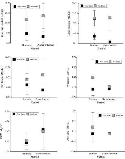
Figure 9: Comparison of mean total fuel load estimations and SD by collection method and fuel type before and after burning.
Post Burn Pre Burn
Biomass Planar Intersect Method 1.53 9.90 18.27 26.63 35.00 T o ta l F u el L o ad in g (M g /h a)
Post Burn Pre Burn Post Burn Pre Burn
Biomass Planar Intersect
Method 0.11 4.66 9.21 13.76 18.31 Li tt er l o ad in g ( M g /h a)
Post Burn Pre Burn
Post Burn Pre Burn
Biomass Planar Intersect
Method 0.25 4.40 8.55 12.70 16.85 D u ff lo ad in g (M g /h a)
Post Burn Pre Burn
Post Burn Pre Burn
Biomass Planar Intersect
Method -0.70 0.17 1.05 1.92 2.79 W ire g ra ss (M g /H a)
Post Burn Pre Burn
Post Burn Pre Burn
Biomass Planar Intersect
Method -1.09 0.69 2.47 4.26 6.04 CW M (M g /h a)
Post Burn Pre Burn
Post Burn Pre Burn
Biomass Planar Intersect
Method -1.00 -0.43 0.15 0.72 1.29 O the r L ive ( M g/ H a)
These graphs help visualizing mean estimations and SD for both methods and all fuel
types; however, conclusions cannot be drawn directly from their interpretation due to the
non-normal distribution of the data and the small sample size.
Bootstrapping was conducted to overcome the small sample size and unknown
distribution. The bootstrapping confidence intervals for the fuel types collected before the
burn overlapped in litter, duff, wiregrass and total fuel estimates; therefore, I concluded that
with a 95% confidence level, both PI and biomass estimates were not significantly different
for pre burn estimations of these fuels (Table 6). However, CWM confidence intervals did
not overlap and therefore the techniques were significantly different in this case. A
comparison was not possible for other live fuels since none were collected with the Planar
Intercept method.
Table 6: Bootstrap summary statistics for all fuel types present before the burn. CL=95% Bootstrap Confidence intervals (α=0.05), n=27, re-sampling size=1,000 Samples marked in red are significantly different.
Confidence intervals of the fuel loading values collected after the burn overlapped in
duff and total load estimations but neither in litter or CWM (Table 7). Therefore, with a 95% Burn status: Pre burn
Fuel Type Mean Std Dev CL Lower CL Upper Mean Std Dev CL Lower CL Upper
Litter 11.510 0.666 10.203 12.803 11.916 1.075 9.874 14.040
Duff 7.506 1.189 5.374 10.116 9.492 1.244 7.316 12.068
Wiregrass 1.049 0.293 0.514 1.644 0.208 0.026 0.158 0.262
CWM 0.844 0.289 0.336 1.379 2.488 0.612 1.469 3.781
Other 0.387 0.155 0.125 0.732 - - -
-Total Fuel 21.313 1.314 18.722 24.137 24.108 2.022 20.286 28.143
Planar Intersect Biomass collection
total fuel loading post burn estimations while they were significantly different for the rest of
the fuel type’s estimations.
On the other hand, the difference in size between confidence intervals by method
(before the burn) were systematically larger in the PI method, suggesting that the variance of
estimating using this method was larger than that resulting from using the Biomass method.
That was not true for estimations after the burn, but it is possible this is due to the small
amount of fuels left after the burn.
Table 7: Bootstrap summary statistics for all fuel types present after the burn. CL=95% Bootstrap Confidence intervals (α=0.05), n=27, re-sampling size=1,000. Samples marked in red are significantly different.
The Wilcoxon-Mann-Whitney test results agreed with all the conclusions obtained in
the previous analysis except post burn duff. Total fuel loads did not show any significant
difference when comparing the loads before and after the burn (pre-burn p-value= 0.5856,
post-burn p-value=0.0933) (Table 8). However, when analyzing the different fuel
components individually before the burn, the test confirmed that litter, duff and wiregrass
load estimates were not significantly different while CWM estimations were significantly
different in both methods (p-value= 0.0103). In this case, duff estimations after the burn were
significantly different between methods (p-value= 0.0475). These results differed with the Burn status: Post burn
Fuel Type Mean Std Dev CL Lower CL Upper Mean Std Dev CL Lower CL Upper
Litter 3.320 0.273 2.817 3.884 0.723 0.073 0.585 0.869
Duff 5.371 0.867 3.894 7.205 3.303 0.479 2.449 4.231
CWM 0.475 0.084 0.317 0.640 2.766 0.546 1.799 3.921
Total Fuel 9.228 1.109 7.179 11.621 6.804 0.881 5.004 8.632
Estimation Method
conclusion obtained with the bootstrapping confidence limits; therefore a third testing (t-test)
was performed following a more traditional approach. The t-test results (p-value= 0.0267)
agreed with the Wilcoxon-Mann-Whitney and I concluded that both methods were
significantly different for post burn duff observations.
Table 8: Wilcoxon-Mann-Whitney U test for significant difference between fuel types collected with two different methods. Methods: Biomass collection=1, Planar Intersect=2, n=27. W=standardized version of the statistic W based on the asymptotic distribution of the same.
Variance values for both methods were also included in the summary statistics. The
high values of the mean variances suggested an over dispersion in all scenarios and pointed
to PI as the method with more variability and therefore less precise.
DISCUSSION
This study indicates that pre bun total fuel loading estimates at burn unit 27 in the
Calloway Forest have a mean value between 21.31 and 24.11 Mg/ha (9.51-10.76 ton/acre)
depending on the estimation method. At a first glance, these values appeared to be high Wilcoxon-Mann-Whitney U test
Burn Status Variable Mean(1) Mean(2) SD(1) SD(2) Var(1) Var(2) W p(2 tails)
Pre Burn Litter 11.53 11.93 3.47 5.81 12.02 33.72 774 0.5856
Duff 7.5 9.5 6.19 6.61 38.26 43.67 639 0.0730
Wiregrass 1.05 0.21 1.59 0.15 2.53 0.02 701 0.4679
CWM 0.85 2.48 1.54 3.24 2.38 10.48 595 0.0103
Other 0.38 0 0.83 0 0.68 0 877.5 0.0006
Total Fuel 21.31 24.11 7.12 10.51 50.76 110.44 691 0.3729
Pos Burn Litter 3.32 0.73 1.47 0.39 2.15 0.15 1097 <0.0001
Duff 5.4 3.27 4.66 2.55 21.73 6.49 857 0.0475
CWM 0.48 2.77 0.45 2.88 0.2 8.27 469 <0.0001
compared with a recent fuel study conducted in the same area (Strand et al. 2013). However,
a deeper analysis of the differences revealed that inventory design, fuel definitions and
measurements were different between studies, especially in duff loadings, and therefore, the
outputs are not comparable. Additional literature reviewed showed that estimations were not
inconsistent with other values found in similar ecosystems with the higher loadings coming
from the litter and duff components (Evans 2012; Lashley 2014; Robertson 2014; Scholl and
Waldrop 1999); 54-49 % and 39-39%, respectively in this study.
Annual litterfall in longleaf pine stands older than 20 years has been estimated to be
about 4.8 Mg/ha (2.14 ton /acre) (Gresham 1982; Roise et al 1991), which corresponds with
litter loads found after 3 years in the study area (11.5 Mg/ha (5.1 ton/acre)). In addition to
this load, it is important to consider the litter decay rates and presence of unburned litter from
the last burn (Bale 2009). When modeling litter accumulation rates after a fire (Olson 1963),
fire behavior (Behave plus software) or fire effects (FOFEM & Consume software), total
combustion of the litter mass is assumed, but this only occurs in the most intensive fires. The
burn management of this unit during the last 11 years has been based on frequent low
intensity fires and therefore, it is expected to have litter left unburned from the last fire. On
the other hand, burns had been conducted in the dormant season, with relative high moisture
and ash content in the duff layer, especially in the lower duff, that would translate in low
smoldering consumption rates of the organic matter (Garlough and Keyes 2011). This is
congruent with the results observed, where around half of the available duff was left
unburned (3 to 5 Mg/ha (1.5-2.5 ton/acre)). Hence, amount of duff in the unit, although not
accumulations, decay conditions, variable relative humidity and ash content of the proper
duff layer. Considering these factors, previous research and that both methods yielded close
estimates; I consider the overall fuel loadings estimates in this study to be a representation of
the fuel mass, with some errors and limitations due to sampling mistakes and personal bias.
However, I recommend treating the duff load estimations with caution, since measurements
related to them have higher uncertainty and inaccuracy.
Comparison between biomass collection and planar intersect (PI) estimates showed
that the two methods were not significantly different when estimating total fuel loadings
before (p-value = 0.3729) and after burning (p-value = 0.0933) but they had significant
differences in estimations of individual fuel types. Previous research has showed that the
biomass collection method is the most precise when estimating continuous fuel loads;
however, its precision decreases as the spatial variation of the fuels increases (Catchpole and
Wheeler 1992). This is consistent with the results of this comparison, with the biomass
estimates being more precise (smaller variance) when estimating continuous fuels.
When analyzing litter loads, pre burn results showed that the two methods’ mean
values were close, what suggests that they have similar estimation capabilities when
measuring horizontally continuous fuels. However, ultimately, the precision of the PI
estimation is going to depend on how appropriate the bulk density is for transforming the
field data into mass estimations (Harmon et al. 2008; Keane and Gray 2013; Parresol et al.
2006; Woodall and Monleon 2006). In this case, the similarity between results points to the
Differences between duff load estimations before and after burning were 2 Mg/ha
(0.89 ton/acre), with the highest value reported by the PI method. This difference almost
corresponds with the amount of ash content subtracted from the biomass samples in the
laboratory. When measuring duff depths in the field following PI method, it was observed
that at some point lower duff and sand were mixed; however, to mark that limit in a
consistent way was complicated and ultimately depended on the field technicians. Similarly
than with litter, total depth was transformed to biomass by multiplying the value by a bulk
density conversion factor (Parresol et al. 2006); which means that a minimum depth
overestimation can yield a huge increase of the load at the landscape level. For example,
knowing that the duff bulk density conversion factor is 7.5310 tons/acre/inch, 1 tenth of an
inch mistake (0.1”) will result in 0.75 ton/acre or 1.69 Mg/ha overestimation at the landscape
level. Therefore, when considering duff load estimates, some level of uncertainty should be
taken into account due to inaccuracy in depth measurements and % of ash content.
Wiregrass estimates before the burn were not significantly different between
methods; however, both sampling methods had significant limitations and it is suggested to
review these values in future work. Some authors have pointed out that when collecting
biomass samples, the precision of the estimates obtained from the sampling decreases as the
spatial variation of the vegetation increases (Catchpole and Wheeler 1992). Wiregrass
naturally distributes in a patchy pattern and giving the sampling size and limitations of the
method, it is probable that the error in generalizing to a large area could have been
substantial. The line intersect areal percentage coverage measured in the 3 transects from the
measured, it was not possible to find adequate equations to transform those percentages into
mass. Equations developed for western species were used (Mitchell et al. 1987) and
therefore, estimations might not reflect the reality of the unit.
A similar problem might be reflected in the CWM estimations of the biomass
method. The distribution and abundance of these types of fuels was better captured with the
sampling design of the PI. In fact, Brown’s method is used in many established fuel sampling
protocols as the most appropriate for sampling CWM (Lutes et al. 2006; National Park
Service 2003; Sikkink and Keane 2008; Woodall and Monleon 2008; Woodall and Williams
2005). An extensive literature review was conducted to find the appropriate quadratic
diameters (Woodall and Monleon 2010), density and decay classes (Woodall and Monleon
2008; Woodall and Williams 2005) to convert the field data into mass values and therefore, I
recommend their use for future work related with longleaf.
Post burn fuel load estimates for both methods corroborated previous statements and
pointed to some interesting variability due to the natural dynamics of the ecosystem. Between
inventories and after the fire, several bad weather episodes (snow, wind and rain) happened,
altering the amount and distribution of the fuels. This was observed in the post burn
inventory where unburned litter had been washed away by a storm the night after the burn.
Both methods estimates reflect this episode but in a different way. The biomass sample was
able to capture a bigger representation of the floor and therefore areas where fuels had been
washed away were complemented with “extra” accumulations of litter. On the contrary, the
PI method is based on measurements at specific points that, if affected by the water, might
3.32 Mg/ha reported for the biomass collection and 0.73 Mg/ha by the PI. Evidence of
alterations due to weather were also evident in the CWM (PI method), which estimates were
higher after the burn than before (2.7 vs. 2.4 Mg/ha).
A deeper analysis of both sampling techniques and estimates has shown that even
though total fuel loading estimates with both methods might not be significantly different;
each method has different precision, strengths and weaknesses. It is important to consider
that every method requires a different amount of money, time, equipment and training; these
considerations might be the ultimate constraint when making a decision from a management
point of view. In general the biomass sampling method is more precise, but it is more
expensive and requires more time and training. Conversely, the PI method is less precise, but
more economical and faster. To choose one method over the other in a fuel sampling
monitoring program, will involve important tradeoffs between precision, time, money,
training, scale, and effectiveness (Sikkink and Keane 2008) and the decision should be driven
by the management goals and resources.
CONCLUSIONS AND MANAGEMENT RECOMENDATIONS
Differences in total fuel load found among the two methods tested in this study are not
large enough to say that they are significantly different; but, there are significant
differences in terms of individual fuel types estimations, adequacy of the method and
sampling efficiency related with cost, time and resources. Agreeing with Sikkink and
Keane (2008) recommendations, I suggest land managers establish an acceptable