SLiM: Simulating Evolution with Selection and Linkage

(1)

NOTE

SLiM: Simulating Evolution with Selection

and Linkage

Philipp W. Messer1 Department of Biology, Stanford University, Stanford, California 94305

ABSTRACTSLiM is an efﬁcient forward population genetic simulation designed for studying the effects of linkage and selection on a chromosome-wide scale. The program can incorporate complex scenarios of demography and population substructure, various models for selection and dominance of new mutations, arbitrary gene structure, and user-deﬁned recombination maps.

R

ECENT studies suggest that linkage effects such as genetic draft and background selection can profoundly alter the patterns of genetic variation in many species (Sella et al.

2009; Lohmueller et al.2011; Weissman and Barton 2012; Messer and Petrov 2013). Understanding the potential im-pact of these linkage effects on population genetic methods requires efﬁcient forward simulations that can model the evo-lution of whole chromosomes with realistic gene structure.

Forward simulations have a long-standing tradition in population genetics and many programs have been developed (Carvajal-Rodriguez 2010; Hobanet al.2011). For any such program, there is typically a trade-off between efﬁciency and

ﬂexibility. Simulations based on combined forward-backward approaches, such as MSMS (Ewing and Hermisson 2010), can be very fast but remain limited to scenarios with only a single selected locus. Current programs that can model scenarios with multiple linked selected polymorphisms, such as FRE-GENE (Chadeau-Hyamet al.2008), GENOMEPOP (Carvajal-Rodriguez 2008), simuPOP (Peng and Kimmel, 2005), forwsim (Padhukasahasram et al. 2008), or SFS_CODE (Hernandez 2008), either lack the ability to model realistic gene structure or are not efﬁcient enough to allow for simulations on the scale of a whole chromosome in reasonably large populations.

Here I present SLiM, a population genetic simulation tar-geted at bridging the gap between efﬁciency andﬂexibility for the simulation of linkage and selection on a chromosome-wide scale. The program can incorporate complex scenarios

of demography and population substructure, various models for selection and dominance, realistic gene structure, and user-deﬁned recombination maps. Special emphasis was further placed on the ability to model and track individual selective sweeps—both complete and partial. While retain-ing all capabilities of a forward simulation, SLiM utilizes sophisticated algorithms and optimized data structures that enable simulations in reasonably large populations. All these features are implemented in an easy-to-use C++ command line program. The source code is freely available under the GNU General Public License and can be downloaded from http://www.stanford.edu/~messer/software.

SLiM simulates the evolution of diploid genomes in a population of hermaphrodites under an extended Wright– Fisher model with selection (Figure 1A). In each generation, a new set of offspring is created, descending from the indi-viduals in the previous generation. The probability of becom-ing a parent is proportional to an individual’sﬁtness, which is determined by the selection and dominance effects of the mutations present in its diploid genome. Gametes are gener-ated by recombining parental chromosomes (both crossing over and gene conversion can be modeled) and adding new mutations.

Mutations can be of different user-defined mutation types, specified by their dominance coefficients and distributions of

fitness effects (DFE); examples could be synonymous, adaptive, and lethal mutations. The possibility to specify arbitrary dominance effects allows for the simulation of a variety of evolutionary scenarios, including balancing selection and re-cessive deleterious mutations. Genomic regions can be of dif-ferent user-defined genomic element types, specified by the particular mutation types that can occur in such elements and their relative proportions; examples could be exons and introns.

Manuscript received April 11, 2013; accepted for publication May 20, 2013 Supporting information is available online athttp://www.genetics.org/lookup/suppl/ doi:10.1534/genetics.113.152181/-/DC1.

1_{Address for correspondence: Department of Biology, Stanford University, 371 Serra}

(2)

Each mutation has a speciﬁed position along the chro-mosome but remains abstract in the sense that the simula-tion does not specify the particular nucleotide states of ancestral and derived alleles. Note, however, that the user has the freedom to associate abstract mutation types with speciﬁc classes of events. There are no back mutations in the simulations. Fixed mutations are removed from the popula-tion and recorded as substitupopula-tions.

SLiM is capable of modeling complex scenarios of de-mography and population substructure. The simulation can include arbitrary numbers of subpopulations that can be added at user-deﬁned times, initialized either with new individuals or with individuals drawn from another sub-population to model a sub-population split or colonization event. Subpopulation sizes, migration rates, and selﬁng rates can be changed over time.

To establish genetic diversity, simulationsﬁrst have to go through a burn-in. Alternatively, simulations can be initialized with a set of predeﬁned genomes provided by the user or with the output of a previous simulation run. The user can further specify predetermined mutations to be introduced at certain time points. Such mutations can be used, for example, to investigate individual selective sweeps or to track the frequency trajectories of particular mutations in the population. Predeter-mined adaptive mutations can also be limited to partial selective sweeps, where positive selection ceases once the mutation has reached a particular population frequency.

SLiM provides a variety of output options, including (i) the complete state of the population at speciﬁed time points,

in terms of all mutations and genomes present in the population; (ii) random samples of specific sizes drawn from a subpopulation at given time points; (iii) lists of all mutations that have becomefixed, together with the times when each mutation became fixed; and (iv) frequency trajectories of particular mutations over time.

I ran SLiM under various test scenarios to check whether its output agrees with theoretical predictions. Speciﬁcally, I analyzed levels of neutral heterozygosity under different scenarios of demography, population substructure, and self-ing, theﬁxation probabilities of new mutations of different selective effects, and the reduction in neutral diversity around adaptive substitutions. Simulation results conformed with the respective theoretical predictions in all tests (Supporting Information,File S1, section 6).

SLiM utilizes sophisticated algorithms and optimized data structures to achieve its high computational efﬁciency (File S1, section 7.1). The simulation is based on a hierarchi-cal data architecture that minimizes the amount of informa-tion stored redundantly. At many stages of the program, large quantities of random numbers have to be drawn from general probability distributions. To do this efﬁciently, SLiM uses lookup tables that are precomputed only once per gen-eration and then allow one to draw random numbers inO

(1) time. Most algorithms are implemented using fast rou-tines provided in the GNU scientiﬁc library (Galassi et al.

2009).

To evaluate SLiM’s performance I compared its runtime and memory requirements with those of SFS_CODE, a popular

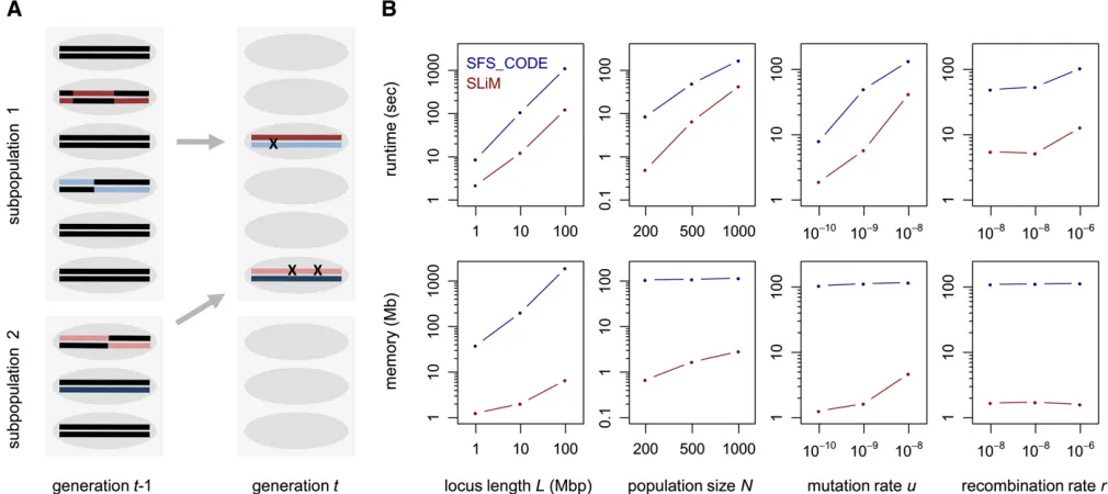
Figure 1 (A) Illustration of SLiM’s core algorithm for a scenario with two subpopulations. In each generation, a new set of offspring is created from the

(3)

forward simulation of similar scope (Hernandez 2008). For these tests, a chromosome of lengthL was simulated with uniform mutation rateuand recombination raterin a pop-ulation of sizeNover the course of 10Ngenerations, assum-ing an exponential DFE with 2Ns ¼ 25 (File S1, section 7.3). The base scenario used values L= 5 Mbp,N= 500,

u = 1029_{, and} _r _{= 10}28 _{per site per generation. I then} varied these four parameters independently to analyze how each individually affects the performance of either pro-gram. Simulations were conducted on a standard iMac desk-top with a 2.8-Ghz Intel core 2 Duo CPU and 4 GB of memory. Figure 1B shows that in all analyzed scenarios SLiM outcompetes SFS_CODE by a substantial margin, typ-ically running 5–10 times faster and requiring 20–100 times less memory. The large discrepancy in memory consumption between the two programs reﬂects the fact that SFS_CODE simulates the sequence of the whole chromosome, whereas SLiM simulates only the actual mutations.

Its computational performance enables SLiM to simulate entire eukaryotic chromosomes in reasonably large popula-tions. For instance, simulating the functional regions in a typical human chromosome of lengthL= 100 Mbp over 105_{generations in a population of size} _N_{= 10}4_with _u₌ 1028_and_r_{= 10}29_{per site per generation, assuming a} func-tional density of 5% and 2Ns ¼ 210, takes 4 days on a single core.

SLiM has already been successfully applied in several projects that required efficient forward simulations on large genomic scales. For example, Kousathanas and Keightley (2013) used the program to examine how linked selection can affect their method for inferring the DFE from polymor-phism data in fruit flies and mice. In Messer and Petrov (2013), SLiM was used to investigate the effects of linked selection on the MK test, and it was shown that such effects can severely bias the test. These studies highlight the need for efficient forward simulations that can model chromo-somes with realistic gene structure.

Most of the current machinery of population genetics is still deeply rooted in the mindset of neutral theory, which assumes that adaptation is rare and that linkage effects from recurrent selective sweeps can thus be neglected. However, this assumption may be violated in many species. It is hence essential to verify with forward simulations under realistic scenarios of selection and linkage whether population genetics methods, and our estimates of key evolutionary parameters obtained from them, are robust to linkage effects. SLiM is speciﬁcally designed for this purpose and I believe that it will become an important tool for future population genetic studies.

Acknowledgments

The author thanks Dmitri Petrov for continuous support throughout the project; members of the Petrov lab, espe-cially Zoe Assaf, David Enard, and Nandita Garud for testing the program; and three anonymous reviewers for their valuable comments on program and documentation. Part of this research was funded by the National Institutes of Health (grants GM089926 and HG002568 to Dmitri Petrov).

Literature Cited

Carvajal-Rodriguez, A., 2008 GENOMEPOP: a program to simu-late genomes in populations. BMC Bioinformatics 9: 223. Carvajal-Rodriguez, A., 2010 Simulation of genes and genomes

forward in time. Curr. Genomics 11: 58–61.

Chadeau-Hyam, M., C. J. Hoggart, P. F. O’Reilly, J. C. Whittaker, M. De Iorioet al., 2008 Fregene: simulation of realistic sequence-level data in populations and ascertained samples. BMC Bioin-formatics 9: 364.

Ewing, G., and J. Hermisson, 2010 MSMS: a coalescent simula-tion program including recombinasimula-tion, demographic structure and selection at a single locus. Bioinformatics 26: 2064_–2065. Galassi, M., J. Davies, J. Theiler, B. Gough, G. Jungman et al.,

2009 GNU Scienti_ﬁc Library: Reference Manual, Ed. 3. Network Theory, Bristol, UK.

Hernandez, R. D., 2008 Aﬂexible forward simulator for popula-tions subject to selection and demography. Bioinformatics 24: 2786–2787.

Hoban, S., G. Bertorelle, and O. E. Gaggiotti, 2011 Computer simulations: tools for population and evolutionary genetics. Nat. Rev. Genet. 13: 110–122.

Kousathanas, A., and P. D. Keightley, 2013 A comparison of mod-els to infer the distribution ofﬁtness effects of new mutations. Genetics 193: 1197–1208.

Lohmueller, K. E., A. Albrechtsen, Y. Li, S. Y. Kim, T. Korneliussen

et al., 2011 Natural selection affects multiple aspects of netic variation at putatively neutral sites across the human ge-nome. PLoS Genet. 7: e1002326.

Messer, P. W., and D. A. Petrov, 2013 Frequent adaptation and the McDonald-Kreitman test. Proc. Natl. Acad. Sci. USA 110: 8615_– 8620.

Padhukasahasram, B., P. Marjoram, J. D. Wall, C. D. Bustamante, and M. Nordborg, 2008 Exploring population genetic models with recombination using efﬁcient forward-time simulations. Genetics 178: 2417–2427.

Peng, B., and M. Kimmel, 2005 simuPOP: a forward-time popu-lation genetics simupopu-lation environment. Bioinformatics 21: 3686–3687.

Sella, G., D. A. Petrov, M. Przeworski, and P. Andolfatto, 2009 Pervasive natural selection in the Drosophila genome? PLoS Genet. 5: e1000495.

Weissman, D. B., and N. H. Barton, 2012 Limits to the rate of adaptive substitution in sexual populations. PLoS Genet. 8: e1002740.

(4)

GENETICS

Supporting Information

http://www.genetics.org/lookup/suppl/doi:10.1534/genetics.113.152181/-/DC1

SLiM: Simulating Evolution with Selection

and Linkage

Philipp W. Messer

(5)

File S1: Supporting Information

Overview

SLiM (Selection on Linked Mutations) is a forward population genetic simulation for studying linkage effects such as hitchhiking under recurrent selective sweeps, background selection, and Hill-Robertson interference. The program can incorporate complex scenarios of demography and population substructure, various models for selection and dominance of new mutations, realistic gene and chromosome structure, and user-defined recombination maps. Special emphasis was further placed on the ability to model and track individual selective sweeps – both complete and partial. While retaining all capabilities of a forward simulation, SLiM utilizes sophisticated algorithms and optimized data structures that enable simulations on the scale of entire eukaryotic chromosomes in reasonably large populations. All these features are implemented in an easy-to-use C++ command line program.

In a forward simulation, every individual in the population is followed explicitly. While this is computationally more intensive than coalescent approaches, it remains a prerequisite for modeling scenarios with multiple linked polymorphisms of different selective effects. Forward simulations have a long-standing tradition in population genetics and many programs have been developed, see [1–3]. For any such program, there is typically a trade-off between efficiency, flexibility, and ease of use. For example, simulations such as msms [4] use a combined forward-backward approach, making them very efficient, yet at the cost that they remain limited to scenarios with only a single selected locus. Other simulations, such as SFS CODE [5], FREGENE [6], forwsim [7], and GENOMEPOP [8] provide high flexibility, but these programs are typically less efficient. Yet other programs such as simuPOP [9] require the user to specify evolutionary scenarios by writing their own scripts in Python. These approaches can provide high flexibility but are complicated to use. SLiM is targeted at bridging the gap between efficiency, flexibility, and ease of use for studying the effects of linked selection.

1 Simulation features

SLiM simulates the evolution of diploid genomes in a population of hermaphrodites. The simulation is based on an extended Wright-Fisher model with selection [10], resembling one of the standard frameworks in population genetics theory [11]. The Wright-Fisher model assumes discrete generations, where the two parents of each child are drawn from the population in the previous generation with probabilities proportional to their fitnesses. Fitness is a function of the mutations present in an individual. Gametes are generated by recombining parental chromosomes and adding new

mutations. Once all offspring are created, they become the parents for the next generation (Figure 1). The fitness

model implemented in SLiM assigns fitnesswi = 1 + 2hisi to individuals heterozygous for the particular mutation i

with selection coefficient si and dominance coefficient hi. Homozygotes for the mutation have fitnesswi = 1 + 2s. A

dominance coefficienth= 0.5, for instance, specifies a codominant mutation,h= 0.1a partially recessive mutation, and

h= 1.2an overdominant mutation. The fitness of an individual is assumed to be multiplicative over all sites: w=Q

iwi.

c

generation t-1 generation t P1

P2

1. 2.

3.

• Calculate the fitnesses of all parents according to the mutations present in their genomes.

• In each subpopulation:

1. For every child, draw two individuals from the parent generation. The probability for an individual to be drawn is proportional to its fitness.

2. Generate gametes by recombining parental chromosomes and add new mutations according to the specified mutational parameters.

3. For the fraction of children that are supposed to be made up by migrants from other subpopulations, draw the parents from the respective subpopulations.

• Make children the new parents for the next generation.

(8)

Mutations can be of different abstract mutation types to be defined by the user. Examples could be synonymous mutations, adaptive mutations, and lethal mutations. A mutation type is specified by the distribution of fitness effects

(DFE) and the dominance coefficient. Genomic regions can be assigned to different user-defined genomic element

types. Examples could be exon, intron, and UTR. A specific genomic element type is defined by the different mutation

types and their relative proportions that can occur in these elements. Thechromosome organizationis finally defined

by the locations of specific genomic elements along the chromosome.

Each mutation has a specified position along the chromosome. SLiM allows more than one mutation to be present in one individual at the same site and there are no back-mutations. Mutations remain abstract entities in the sense that the simulation does not specify the actual nature of a mutation, such as the particular nucleotide states of ancestral and derived alleles or whether the mutation is a single nucleotide mutation, an insertion or deletion, an inversion, etc. Note, however, that the user always has the freedom to associate abstract mutation types with specific classes of events.

As an illustration of the concept of mutation types and genomic element types, consider the following example: Suppose one intends to model the evolution of exons under recurrent selective sweeps and background selection. In this case, one could define three different mutation types: ‘synonymous’, ‘deleterious’, and ‘adaptive’. The synonymous mutations

would all be assigned a fixed selection coefficients= 0. The selection coefficient of the deleterious mutations could be

drawn from a gamma distribution with means=−0.05, shape parameterα= 0.2, and dominance coefficient h= 0.2.

The adaptive mutations would be modeled with fixed selection and dominance coefficients, says= 0.001 andh= 0.5.

The single genomic element type in this example would be ‘exon’, defined by the presence of all three mutation types with relative proportions 0.25 for synonymous mutations, 0.74 for deleterious mutations, and 0.01 for adaptive mutations. The chromosome organization would finally be specified by the locations of exons along the chromosome.

Therecombination modelimplemented in SLiM can incorporate both crossing-over and gene-conversion. Recombination events during meiosis are drawn from a user-specified recombination map. The ratio between gene conversion and crossing over can be specified by the user, as can be the average length of gene conversion tracts.

SLiM can model complex scenarios ofdemographyandpopulation substructure. The simulation allows for arbitrary

numbers of subpopulations to be added at user-defined times, either initialized with new individuals, or from the individuals drawn from another subpopulation to model a population split or colonization event. The size of each subpopulation can be changed at any time to model demographic events such as population bottlenecks or expansions. The rates of

migration between any two subpopulations can be specified or changed by the user at any time. The simulation also

allows to modelselfingby specifying selfing rates that can vary over time and between subpopulations.

The simulation keeps track of all mutations that become fixed in the population over the course of a run. Once fixed,

such mutations are removed and recorded as substitutions, as they can no longer cause fitness differences between

individuals. However, in scenarios with more than one subpopulation, only the mutations that have become fixed in all subpopulations are removed.

A simulation run starts with empty genomes. In order to establish genetic diversity, simulations first have to undergo a burn-in period. Alternatively, SLiM can be initialized from a set of pre-defined genomes provided by the user. This can also be the output from a previous simulation run.

The user can specify predetermined mutations to be introduced at specific time points in a simulation run. Such

mutations can be used, for example, to investigate individual selective sweeps or to track the frequency trajectories of

specific mutations in the population. Predetermined adaptive mutations can further be assigned to undergo onlypartial

selective sweeps, where positive selection ceases once the mutation has reached a predefined population frequency.

SLiM provides several options for theoutputof its simulation results: (i) Output of the complete state of the population

(9)

2 Installation

SLiM is a command line program written in the C++ programming language. The source code ‘slim.cpp’ can be downloaded from http://www.stanford.edu/∼messer/software. To compile the program, it is recommended to use the GNU gcc compiler, which should be installed on most Unix-type operating systems. On Mac OS X, the gcc compiler is not installed by default but is freely available in the xcode suite of development tools. To install the gcc compiler on Mac OS X, first download and then install the xcode package from http://connect.apple.com. SLiM also requires the GNU scientific library (GSL) [12], which provides essential routines for the algorithms implemented in the simulation. GSL should already be installed on many systems, but may need to be installed manually on some systems. To check whether GSL is already installed on your system, type in your command-line terminal (Windows users should download and install Cygwin from http://www.cygwin.com or another such application):

$ gsl-config

This command should return a usage description and a list of options if GSL is properly installed. A quick tutorial for installing GSL on Linux, Mac OS X, or Windows is provided at http://www.brianomeara.info/tutorials/brownie/gsl. To compile SLiM, change into the directory where the source code is located and type:

$ g++ -O3 ./slim.cpp -lgsl -lgslcblas -o slim

On Mac OS X, the option-O3, which specifies the optimization level applied by the compiler, should be replaced with

-fast. The options-lgsland-lgslcblaslink the program with the GSL library.

3 Running SLiM

SLiM is a command line program. The parameters for a simulation run have to be provided to the program in the form of a standardized parameter file (we chose to use a parameter file instead of command line arguments for reasons of comprehensibility when complex evolutionary scenarios with many parameters are simulated). To run the simulation with

the parameter file<filename>, type:

$ ./slim <filename>

The parameter file is a standard text file. Each line preceded by ‘#’ in this file indicates that in the following section,

until either the next occurrence of a line preceded with ‘#’ or the end of the file, a specific parameter will be defined.

The following parameters can be specified:

#MUTATION TYPES

#MUTATION RATE

#GENOMIC ELEMENT TYPES

#CHROMOSOME ORGANIZATION

#RECOMBINATION RATE

#GENERATIONS

#DEMOGRAPHY AND STRUCTURE

#OUTPUT (optional)

#GENE CONVERSION (optional)

#PREDETERMINED MUTATIONS (optional)

#INITIALIZATION (otional)

#SEED (optional)

Comments can be added throughout the parameter file by preceding a comment with ‘/’, in which case all subsequent

(10)

4 Simulation parameters

4.1 Mutation types and mutation rate

Mutation types are specified by the DFE from which the selection coefficients of mutations of this type are drawn and their dominance coefficient. The syntax for defining mutation types is:

#MUTATION TYPES

<mutation-type-id> <h> <DFE-type> [DFE parameters]

...

The<mutation-type-id>is used to identify the mutations of this type and can be any number preceded by the letter ‘m’,

for examplem4. This id will be used to specify the mutation types that are present in a particular genomic element type.

The value of<h>specifies the dominance coefficient assigned to mutations of this type, for example0.5for codominant

mutations or0.1for partially recessive mutations.

<DFE-type>specifies the DFE from which the selection coefficients of mutations of this type are drawn, followed by the

specific parameters needed to define the particular DFE. Possible DFE types are:

1. fixed selection coefficient: f <s>

2. exponential distribution: e <mean-s>

3. gamma distribution: g <mean-s> <shape-alpha>

Under the exponential DFE, selection coefficients are drawn from a probability density P(s|s) = s−1_{exp (}_−s/s₎_{. An}

exponential DFE is often used to model advantageous mutations [13]. Under the gamma DFE, selection coefficients are

drawn from a gamma distribution with probability density P(s|α, β) = [Γ(α)βα_]−1_exp(_−s/β₎_{. The shape parameter}

αspecifies the kurtosis of the distribution. The mean of the distribution is given by s =αβ. A gamma DFE is often

used to model deleterious mutations at functional sites [13]. Note that selection coefficients are always defined in terms of their absolute values and not multiplied by an effective population size.

The simulation assumes a uniform mutation rate<u>per nucleotide per generation along the chromosome that is set by

the parameter:

#MUTATION RATE

<u>

The mutation rate can be specified in either decimal or scientific e-notation (for example2.5e-8).

4.2 Genomic element types

A genomic element type is specified by a list of mutation types and their relative proportions in the elements of this type. An example of a genomic element type would be ‘exon’, defined by the presence of ‘synonymous’ and ‘nonsynonymous’ mutations and their respective proportions. The syntax for defining genomic element types is:

<element-type-id> <mut-type> <x> [<mut-type> <x> ...]

...

The<element-type-id>can be any number preceded by the letter ‘g’, for exampleg2. This id will be used for specifying

the chromosome organization in terms of the locations where genomic elements of a specific type are located along the chromosome.

Each following pair of numbers specifies a particular mutation type <mut-type> and its relative proportion <x> among

the mutations in this genomic element type. The proportions do not actually have to add up to one and are interpreted

relative to each other (mutations always occur at the per-site rate specified in#MUTATION RATE). For example, the genomic

(11)

g1 m4 0.5 m3 1.0

comprises mutations of types m4andm3, with the mutations of typem3 occurring twice as often as those of typem4.

4.3 Chromosome organization

The organization of the chromosome is specified by the locations of genomic elements along the chromosome. The syntax for defining the chromosomal organization is:

<element-type> <start> <end>

...

Each line represent a genomic element, specified by its<element-type> and followed by its<start>and<end>position

on the chromosome in base pairs. The specified genomic regions do not have to cover the entire chromosome, but mutations will only occur in the regions that have been specified. Thus, one can easily model the evolution of only a subset of regions on a chromosome. Genomic elements do not need to be specified in the same order as they are located along the chromosome. However, overlap between genomic regions is not permitted.

4.4 Recombination

SLiM allows the user to specify arbitrary recombination rates that are also allowed vary along the chromosome. Recom-bination rates are specified by the syntax:

#RECOMBINATION RATE

<interval-end> <r>

...

The first row specifies the recombination rate from the start of the chromosome up to the position specified by

<interval-end>. In subsequent rows, the recombination rates for consecutive intervals can be specified. The

recombi-nation rate <r> for a particular interval is defined in terms of recombination events per nucleotide per generation and

can be specified in either decimal or scientific e-notation. Note that the commonly used unit of 1 cM/Mb corresponds

to a per nucleotide recombination rate of 1e-8. Intervals have to be defined in ascending order and the end of the last

interval should extend up to the end of last genomic element defined in the chromosome organization, as recombination rate will automatically be set to zero to the right of the last specified interval. Recombination rates can be specified in

either decimal or scientific e-notation (for example1.5e-7).

4.4.1 Crossing over and gene conversion

By default, every recombination event results in a crossing over of the two parental chromosomes during meiosis (Figure 1). Optionally, a fraction of recombination events can be specified to result in gene conversion. Gene conversion is modeled by excising a genomic conversion stretch of a particular length to the right of the recombination breakpoint. The length of the conversion stretch is drawn from a geometric distribution. The syntax for modeling gene conversion is:

#GENE CONVERSION

The parameter <fraction> specifies the probability that a recombination event results in gene conversion rather than

crossing over. In the remainder of events, recombination still leads to crossing-over. <stretch-length> specifies the

(12)

4.5 Demography and population structure

The number of generations<t>for which the simulation is to be run is set by the parameter:

#GENERATIONS

<t>

Time is specified in actual generations and not rescaled by any sort of effective population size. In contrast to many coalescent simulations, time is also specified in the forward direction; that is, a simulation run starts in generation one

and ends after generation<t>.

By default, at the start of a simulation run all genomes in the population are empty since no mutations have yet occurred. Therefore, simulations have to undergo a burn-in period in order to establish the required levels of genetic diversity. For

neutral mutations, as a rule of thumb, evolution typically needs to be simulated for10Ne generations in order to obtain

stationary levels of neutral polymorphism, whereNe is the variance effective population size over the initial time period

in the specific evolutionary scenario. Stationary levels of polymorphism for deleterious and advantageous mutations can be approached considerably faster.

Demography and population structure is modeled by specifying events such as the introduction of a new subpopulation or the change of a subpopulation’s size at specific time points. The general syntax for specifying such events is:

<time> <event-type> [event parameters]

...

The first parameter,<time>, specifies the particular generation in which<event-type>will be executed, followed by a list

of parameters for the particular event. Events do not have to be specified in the same order as they occur; they will be sorted automatically by the program. Events are always executed at the beginning of a generation. For example, changing

the size of a subpopulation from N1 toN2 in generationt implies that N2 children will be generated in generationt.

Events can be of three different types, which will be discussed in order below:

adding new subpopulation: <time> P <pop> <N> [<source-pop>]

changing population size: <time> N <pop> <N>

changing migration rate: <time> M <target-pop> <source-pop> <m>

changing selfing rate: <time> S <pop> <σ>

4.5.1 Adding new subpopulations and modeling population splits

An event of type ‘P’ adds a new subpopulation of size <N> with identifier <pop> in generation<time>. The syntax for

introducing a new subpopulation is:

<time> P <pop> <N> [<source-pop>]

The identifier<pop>of the new subpopulation can be any number preceded by the letter ‘p’, for examplep3. The identifier

values for different subpopulations do not need to be in any particular order. By default, the new subpopulation consists of individuals with empty genomes; that is, no mutations are yet present. Alternatively, the new subpopulation can be

initialized with individuals drawn from an already existing subpopulation <source-pop>, allowing to model population

splits and colonization events. In this case, the probability of being chosen as a migrant is proportional to an individual’s fitnesses in the source population. Note that migrants are not actually removed from the source population, they will rather be used as parents when generating the children in the new subpopulation (Figure 1).

Importantly, all simulations should start with an event of the form ‘1 P <pop> <N>’, unless an initialization file is provided

(see section 4.9). This introduces an initial population of size<N>in the first generation. Figure 2 shows an illustration

(13)

N1

N3 N2

t1 t2 t3

<t3> P p3 <N3> p1

Figure 2. Illustration of the ‘P’ event type. Subpopulation p1 of size <N1> is created in generation<t1>and subpopulationp2of size<N2>in generation<t2>. In generation<t3>, subpopulationp3splits off fromp1.

4.5.2 Changing population sizes and deleting subpopulations

An event of type ‘N’ sets the size of subpopulation<pop>to<N>in generation<time>. The syntax for setting population

size is:

If the size of a particular subpopulation is set to zero, this subpopulation is deleted and all migration rates from or to this subpopulation are also reset to zero. Population size changes are always executed at the beginning of a generation. In the Wright-Fisher model, population size changes are treated as ‘instantaneous’ events by adjusting the number of

N1 N2 N3

t1 t2 t3

Figure 3. Illustration of the ‘N’ event type. Subpopulationp1of size<N1>is created in generation<t1>. In generation <t2>, its population size is reduced to <N2> but recovers in generation<t3>to size<N3>.

children that are generated in subsequent generations. If a continuously changing population size is to be modeled, the population sizes have to be specified explicitly for each generation.

Note that when population sizes are changed, selection coefficients are not rescaled, as sometimes done in other forward simulations. Thus, an increase in population size can lead to stronger effective selection and vice versa. Figure 3 shows

an illustration for the usage of the ‘N’ event type to simulate a simple bottleneck scenario.

4.5.3 Migration and admixture

An event of type ‘M’ sets the migration rate from the source population<source-pop>to the target population<target-pop>

to the value<m>in generation<time>. The syntax for this event type is:

The value of<m>specifies the fraction of individuals of the target population that will be made up of migrants from the

(14)

Note that in the Wright-Fisher model, migrating individuals are not actually removed from the source population, they will rather be used as parents when generating the children in the target population (Figure 1). Migration has therefore no effect on actual population sizes. However, when setting migration rates, it needs to be assured that for any subpopulation

the sum of the overall fractions of migrants from other subpopulations, Mi =Pjmij, never exceeds one. Events of

type ‘M’ can also be used to model population admixture, as shown in Figure 4.

N1

N3 N2

t1 t2 t3

m31 m21 m12

<t2> P p3 <N3> p1

<t3> M p1 p2 0.5

<t3+1> N p2 0

Figure 4. Illustration of the ‘M’ event type. In gen-eration <t1> two subpopulations p1 and p2 are cre-ated. The migration rate is set to <m21> from p1 to p2 and <m12> in the other direction. In gener-ation <t2>, subpopulation p3 splits off from p1 and migration fromp1top3is set to rate<m31>. In gen-eration<t3>, subpopulationp2admixes with subpop-ulation p1, implemented by setting the fraction ofp1 made up by migrants fromp2to0.5for that particu-lar generation, and then eliminatingp2by setting its size to0in the following generation.

4.5.4 Self-fertilization

SLiM assumes random mating by default. However, some species, such as certain plants, can also reproduce through selfing. This can be simulated in SLiM by specifying the probability that a child results from self-fertilization rather than

from random mating. To do this, one has to specify an event of type ‘S’, which sets the selfing rate in population<pop>

to the value<σ>in generation<time>. The syntax for this event type is:

<time> S <pop> <σ>.

A value<σ>=1specifies a subpopulation that reproduces exclusively through selfing, whereas<σ>=0.5specifies a scenario

where both selfing and outcrossing occur equally likely. The default selfing rate, if not otherwise specified, is <σ>=0.

Note that this implementation allows the user to change the selfing rate over time and also to have different selfing rates in different subpopulations.

4.5.5 Remarks on complex demographic scenarios

While SLiM is designed to allow for arbitrarily complex scenarios of demography and population substructure, one needs to be aware that the directives required for specifying such scenarios can quickly become difficult to follow. This raises the potential for inconsistent directives, for instance, changing the size of a subpopulation that is not actually present. In most of the situations where inconsistent directives are encountered, SLiM will exit with an error message reporting the particular type of problem. However, it is important to keep in mind that some of these problems might only show up during the simulation. The list of directives is not checked for consistency prior to the simulation. Thus, computation time might be lost if the problem is encountered only after the program has already been running for some time. To prevent this from happening, it is strongly recommended that prior to running long simulations, initial test runs are conducted to check the list of directives for consistency. The mutation rates, recombination rates, and population sizes in these test runs can be set to small values so that the simulation finishes quickly.

4.6 Output

Specifying the output of simulation results is handled in a similar fashion to the specification of demographic events

described in the previous section. For each requested output, the user has to specify the <time> at which the output

should be returned, the particular <output-type>, and the required parameters for this type of output in the #OUTPUT

(15)

#OUTPUT

<time> <output-type> [output parameters]

...

The following types of output can be requested from the simulation and each type will be discussed in detail with the help of examples in a subsequent section:

Output state of entire population: <time> A [<filename>]

Output random sample from subpopulation: <time> R <pop> <size>

Output list of all fixed mutations: <time> F

Track mutations of particular type: <time> T <mut-type>

Before any such user-specified output is provided, the simulation first prints the input parameters of the particular run, including the value of the seed used for the random number generator (see section 4.10). For instance, the initial output for the simple neutral scenario from section 5.1 will look as follows:

#INPUT PARAMETER FILE

./input example 1.txt

#MUTATION TYPES

m1 0.5 f 0.0

#MUTATION RATE

1e-8

g1 m1 1.0

g1 1 100000

#RECOMBINATION RATE

100000 1e-8

#GENERATIONS

10000

1 P p1 500

#OUTPUT

10000 R p1 10

10000 F

#SEED

1346284673

Note that from this initial output it is possible to reproduce the particular simulation run exactly, since all simulation runs with the same simulation parameters starting with the same seed will yield exactly the same simulation output (see section 4.10).

User-requested output will be printed whenever the simulation run has reached the specific time point for which the

output is requested. Each such output starts with a line ‘#OUT: <time> <output-type> [output parameters]’, followed

by the particular output in the subsequent lines.

4.6.1 Output entire population

The output type ‘A’ returns the complete state of the population at the end of generation<time>. Optionally the output

will not be printed on the screen but instead written into the file<filename>. The syntax is:

<time> A [<filename>]

(16)

output obtained using the ‘A’ option after generation 20 in a simulation run with two small subpopulations, consisting of two individuals each. On the right, short explanations for the particular output lines are given:

#OUT: 20 A

Populations:

p1 2

p2 2

Mutations:

1 m2 7149 -0.00364166 0.2 3

2 m2 6181 -0.00715424 0.2 4

3 m2 8179 -0.009072 0.2 2

4 m1 5636 0 0.5 1

Genomes:

p1:1 1

p1:2 1

p1:3

p1:4 1

p2:1 4 2 3

p2:2 2

p2:3 2 3

p2:4 2

Header:

List of all populations: <pop> <N>

...

List of all mutations:

<id> <type> <x> <s> <h> <n> ...

... ...

List of all genomes:

<pop:genome> <id> ...

... ... ... ... ... ... ...

The sectionPopulations lists all subpopulations. Each subpopulation is denoted by its population identifier<pop>and

size<N>in terms of numbers of diploid individuals.

The following section,Mutations, lists all mutations that are polymorphic in the population. Each mutation is assigned

a unique<id>in ascending order that is used to identify this particular mutation in the genomes that carry it. Note that

mutation ids are not necessarily kept constant between generations; the same mutation will likely be assigned a different

id in another generation. Each mutation is further described, in order, by its mutation type <type>, position <x> on

the chromosome, selection coefficient<s>, dominance coefficient<h>, and the overall number<n>of genomes carrying

this mutation. Note that the output of the mutation prevalences for each mutation provides an easy way to calculate polymorphism frequency distributions.

The last list,Genomes, specifies all genomes in the population. Each line is a genome. The starting string<pop:genome>

specifies the subpopulation identifier<pop>, followed by a number used to enumerate the genomes of this subpopulation

in ascending order. Genomes can easily be mapped onto individuals as individuali has the two genomes2i−1and2i.

The subsequent numbers list the<id>values of the different mutations present in the particular genome. For example,

the line ‘<p2:1> 4 2 3’ specifies genome 1in subpopulationp2and this genome carries the mutations 4,2, and3.

4.6.2 Output random sample from a subpopulation

The output type ‘R’ returns a sample of <size> genomes drawn randomly from subpopulation <pop> at the end of

generation<time>. The syntax is:

All genomes present in the population have equal probability of being drawn and the same genome can be drawn several

times. The following is an example for the output obtained with the ‘R’ option when requesting a random sample of4

(17)

#OUT: 10 R p1 4

Mutations:

1 m1 2383 0 0.5 3

2 m1 9828 0 0.5 3

3 m1 211 0 0.5 1

4 m2 7576 -0.0186089 0.2 1

Genomes:

p1:3 1 2

p1:4 3 4

p1:2 1 2

p1:1 1 2

Header:

List of all mutations:

<id> <type> <x> <s> <h> <n> ...

... ...

List of all genomes:

<pop:genome> <id> ...

... ... ...

Note that the output style is very similar to the output under the option ‘A’, with the primary difference that only the

mutations and genomes present in the sample are shown. Here, the values of<n>denote prevalences of the mutations in

the sample, not in the whole population.

4.6.3 Output list of all fixed mutations

The program records all mutations that have become fixed over the course of a simulation run and removes these mutations from the populations. This is reasonable because fixed mutations can no longer generate fitness differences

between individuals and back mutations do not occur. The output type ‘F’ returns the list of all mutations that have

become fixed until the end of generation<time>. The syntax is:

<time> F

The following is an example for output obtained with the ‘F’ option in a simulation after 1000 generations:

#OUT: 1000 F

Mutations:

1 m1 6281 0 0.5 23

2 m1 4693 0 0.5 552

3 m1 1261 0 0.5 675

4 m2 2531 -0.002165 0.2 683

5 m1 9458 0 0.5 719

Header:

List of all fixed mutations: <id> <type> <x> <s> <h> <t> ...

... ... ...

The last number in each mutation row,<t>, denotes the generation in which the particular mutation has become fixed.

Note that in scenarios with several supopulations, a mutation has to be fixed in all subpopulations to be recorded and removed. This can slow down scenarios with population substructure and low migration rates if subpopulations accumulate many private mutations.

4.6.4 Track mutations of particular types

SLiM allows to track the frequency trajectories of particular mutations in the population using the output type ‘T’. For

this purpose, one needs to specify the particular mutation type<mut-type>of the mutations that are to be tracked and

the generation<time>at which the tracking is supposed to start. The syntax for the ‘T’ output type is:

In every generation after <time>, the population will then be screened for all mutations of type<mut-type>and every

such mutation will be reported with an output line of the form:

(18)

The value of <n> specifies the prevalence of the particular mutation in the population in <generation>. Note that if

several mutations of the specified<mut-type>are present in the population, a separate output line is provided for each of

those mutations. Thus, if a single mutation is to be tracked, this mutation should be given a unique <mut-type>. This

can easily be attained for predetermined mutations, as described in section 4.7. In scenarios with several subpopulations

<n> specifies the abundance of the mutation in the overall population, not just a particular subpopulation.

4.7 Introducing predetermined mutations

SLiM provides the option to introduce predetermined mutations into the population at user-defined time points and

positions on the chromosome. This option can be used, for example, to investigate selective sweeps or track the

trajectories of specific mutations in the population. There is no limit on the possible number of predetermined mutations. The syntax for introducing predetermined mutations is:

#PREDETERMINED MUTATIONS

<time> <mut-type> <x> <s> <h> <pop> <nAA> <nAa> [P <f>]

...

This directive introduces a mutation of type <mut-type> at genomic position <x> with selection coefficient <s> and

dominance coefficient <h> at the end of generation<time>. The mutation will be added in homozygous form to<nAA>

random individuals and in heterozygous form to another <nAa> random individuals in the subpopulation <pop>. The

optional parameterP <f>can be used to model partial selective sweeps and will be discussed in section 4.8.

Technically, SLiM introduces such mutations to both genomes of the first1,...,<nAA> individuals in the subpopulation

and then to only the first genome of the subsequent<nAA>+1,...,<nAA>+<nAa>individuals in the subpopulation. This is

effectively equivalent to introducing the mutation into random individuals. However, should more than one mutation be introduced in the same generation, they will end up in the same individuals. If full control is needed over which mutations are introduced into which genomes, it is recommended to start the simulation with a user-defined initialization file, where all mutations and genomes can be specified explicitly. This possibility is described in section 4.9.

Note that for predetermined mutation the mutation type does not play the same role it does for regular mutations, where it determines the DFE from which their selection coefficients are drawn and their dominance coefficient. Nevertheless, for predetermined mutations the mutation type can still play a crucial role for identifying a particular mutation in the simulation output and for tracking such mutations. For this purpose, one can assign a unique mutation type to a

predetermined mutation that has not been used already in the#MUTATION TYPESsection of the input parameter file. This

way the predetermined mutation can be tracked individually. Note that<mut-type>can be any number preceded by the

letter ‘m’, for examplem17.

4.8 Simulating complete and partial selective sweeps

One application for predetermined mutations is the possibility to model individual selective sweeps. Furthermore, SLiM

allows to simulate partial selective sweep by specifying the ‘P’ option for a predetermined mutation:

...

In this case, the selection coefficient of the mutation will be set to zero once the mutation has reached population

frequency<f>. Note that in scenarios with several subpopulations<f>refers to the overall frequency of the mutation in

all subpopulations.

When modeling selective sweeps using predetermined mutations, one always has to keep in mind that even a strongly advantageous mutation can still become lost from the population due to random genetic drift. A mutation with selection

coefficient sand dominance coefficient h, when present initially in only one copy, has probability ≈4hsof reaching its

establishment frequency(4hsN)−1 _{in the population, where selection outweighs drift and the mutation is thus unlikely}

(19)

0 500 1000 1500 2000

0.0

0.2

0.4

0.6

0.8

1.0

generation t

frequency

x

x(t ) = 1

1++x0−−

1_{exp(−2h st )} _{Figure 5.} _{Illustration of the trajectory of a partial selective}

sweeps (s= 0.01andh= 0.5) in a population of5×104 individuals with a destined frequency of0.5. The mutation was introduced into 100 heterozygous individuals in the first generation. No other mutations were present. The dashed red line shows the theoretically expected trajectory during the selected phase.

SLiM does not condition on the establishment of predetermined mutations. Thus, if a selective sweep is to be simulated, one has to verify from the simulation output that the mutation has not actually been lost. Since the establishment probability of a advantageous mutation is proportional to the product of its initial frequency, its selection coefficient, and its dominance coefficient, increasing any of these parameters can increase establishment probability.

However, for many analyses the selection and dominance coefficients will be fixed, possibly at values where loss of the mutation is still very common. And increasing the initial population frequency of an advantageous mutation via the

<nAA>and<nAa>parameters can raise the problem that the mutation might then be present on many different genomic

backgrounds, which can be unrealistic when modeling adaptation fromde novomutation.

One possible approach to this problem is to link the mutation to a second ‘booster mutation’ undergoing a partial selective sweep, which raises the first mutation to its establishment frequency but thereafter becomes selectively neutral. For example, consider the following scenario:

100 m1 5000 0.01 0.5 p1 0 1

100 m2 5000 0.25 1.0 p1 0 1 P 0.01

Here two advantageous mutations are introduced at position 5000 in one copy. Since the two mutations are also

introduced in the same generation100, both will actually end up in the same genome (remember that several mutations

can be present at the same site in one genome in SLiM). However, the first mutation has an establishment probability

of only4h1s1= 0.02, whereas the second mutation, which undergoes a partial sweep, has an establishment probability

of4h2s2= 0.5. Hence, in 50% of the runs the second mutation will drag the first mutation to population frequency of

1%, its establishment frequency in a population of sizeN = 500.

Figure 5 demonstrates the ability of SLiM to simulate and track a partial selective sweep with a destined population frequency of 0.5. The frequency trajectory of the mutation during its selected phase agrees with the theoretically expected trajectory for the given selection and dominance coefficients. Once the mutation has reached its destined population frequency, it drifts neutrally

4.9 Initializing the population from a file

By default, at the start of a simulation run all genomes in the population are empty since no mutations have yet occurred. Alternatively, SLiM can be initialized with the populations, mutations, and genomes specified in an initialization file. The format of this initialization file is the same format used for the output of the complete state of the population described in section 4.6.1, that is, a list of all subpopulations and their sizes, all mutations and their parameters, and all genomes present in the population. Any such output file can serve as an initialization file for another simulation run. Note,

however, that only the sections Populations, Mutations, andGenomes are required, while the evolutionary parameters

specified in the header will be ignored. Of course, one can also use a custom initialization file, as long as it contains valid

data in the sections Populations, Mutations, and Genomes. Every genome can then be defined by the user explicitly.

The syntax for initializing a simulation run from the data provided in the file<filename>is:

#INITIALIZATION

(20)

In this case, all populations, mutations, and genomes specified in this file will automatically be carried over into the new

simulation run at the start of generation one. The populations do not need to be added again in the section#DEMOGRAPHY

AND STRUCTUREof the parameter file (doing so would actually cause an error as the particular populations already exist). However, all other evolutionary parameters, such as mutation types, chromosome organization, recombination rate, migration rates, etc., still have to be specified in the parameter file if evolution is to proceed under these parameters. These parameters are intentionally not provided in the initialization file so that the simulation run can be started with different parameters. One should be particularly careful when specifying the parameter file to avoid inconsistencies with the data provided in the initialization file.

Starting a simulation run from an initialization file provides a straightforward way to split up a simulation into different stages. This can can be very useful, for example, when analyzing the reproducibility of evolution under specific scenarios, such as in the example described in section 5.4.

4.10 Random number generator seed

SLiM uses a maximally equidistributed combined Tausworthe random number generator [14]. By default, the seed is a combination of the starting time of the program and its process id. This procedure assures that every time the program is called, a different seed will be used, even if several instances of the program are started simultaneously. Alternatively, a user-defined value for the seed can be specified via:

#SEED

<seed>

The<seed>can be any 4-byte integer number (−231. . .231). Since all simulation runs starting with the same seed will

yield exactly the same output, this option can be very useful when simulation runs have to be reproduced.

5 Examples

5.1 Simple neutral scenario

This example simulates a 100 kbp long genomic region evolving under a uniform mutation rate of u= 10−7 per site

per generation and a uniform recombination rate ofr= 1 cM/Mbp. All mutations are neutral. The population of size

N = 500is simulated over104 _{generations. Samples of 10 random chromosomes are drawn every}₄_N _{generations. At} the end of the simulation, all fixed mutations are reported.

#MUTATION TYPES

m1 0.5 f 0.0 / neutral

#MUTATION RATE

1e-7

g1 m1 1.0 / only one type comprising the neutral mutations

g1 1 100000 / uniform chromosome of length 100 kbp

#RECOMBINATION RATE

100000 1e-8

#GENERATIONS

10000

1 P p1 500 / one population of 500 individuals

#OUTPUT

2000 R p1 10 / output sample of 10 genomes

4000 R p1 10

...

(21)

5.2 Hitchhiking of deleterious mutations under recurrent selective sweeps

In this example we want to analyze the complex dynamics resulting from the interactions between deleterious and beneficial mutations under recurrent selective sweeps. In particular, we are interested in the polymorphism frequency distributions and fixation probabilities of functional mutations.

For this purpose, we simulate the evolution of a chromosome of length 10 Mbp in a panmictic population of constant

size N = 103_{. Functional mutations should occur on each chromosome at a uniform rate of} _u_{= 2}_.₅_×₁₀−9 _{per site}

per generation. The selection coefficients of these functional mutations are drawn from an exponential distribution with

mean s =−0.01, and they are assumed to be partly recessive with a dominance coefficient h= 0.2. However, 1 out

of 2000 mutations is assumed to be adaptive with a selection coefficient s= 0.01 and dominance coefficienth= 0.5.

Recombination occurs uniformly along the chromosome at rater= 1cM/Mbp.

We simulate the evolution of this chromosome for 105 generations. Every 104 generations, a random sample of 50

genomes is drawn from the population. At the end of the simulation run we want to obtain a list of all the mutations that have become fixed. This parameter file for this scenario is:

#MUTATION TYPES

m1 0.2 e -0.01 / deleterious (exponential DFE, h=0.2)

m2 0.5 f 0.01 / advantageous (fixed s=0.01, h=0.5)

#MUTATION RATE

2.5e-9

g1 m1 0.9995 m2 0.0005 / 1 in 2000 mutations is adaptive

g1 1 10000000 / uniform chromosome of length 10 Mbp

#RECOMBINATION RATE

10000000 1e-8 / uniform recombination rate (1 cM/Mbp)

#GENERATIONS

100000

1 P p1 1000 / single population of 1000 individuals

#OUTPUT

20000 R p1 50

...

100000 F / output fixed mutations

5.3 Background selection with gene structure and varying recombination rate

In this third example we want to investigate how background selection affects the patterns of neutral and functional polymorphism under varying recombination rate along a gene. The gene of interest is supposed to resemble an ‘average’ human gene (Figure 6). Mutations in exons are assumed to be neutral (25%) or deleterious (75%), with the selection

coefficients of the deleterious mutations drawn from a gamma distribution with mean s=−0.05 and shape parameter

α= 0.2. The deleterious mutations are assumed to be recessive with dominance coefficient h= 0.1. In UTRs, half of

the mutations are assumed to be neutral, the remainder deleterious with the same selection parameters as used for exons.

exons (150 bp)

introns (1.5 kbp) UTRs (550 bp)

position

re

co

mb

in

at

io

n

ra

te

5.5 kbp 6.5 kbp

r = 1 cM/Mbp r = 2

r = 4

(22)

The mutations in introns are always neutral. We assume a mutation rate of u= 10−8 _{and a recombination profile as}

specified in Figure 6. The population of sizeN = 104 is simulated over 106 generations. To calculate polymorphism

statistics, samples of 100 random genomes are drawn every2N generations. The parameter file for this scenario is:

#MUTATION TYPES

m1 0.1 g -0.05 0.2 / deleterious (gamma DFE, h=0.1)

#MUTATION RATE

1e-8

g1 m1 0.75 m2 0.25 / exon (75% del, 25% neutral)

g2 m1 0.50 m2 0.50 / UTR (50% del, 50% neutral)

g3 m2 1.0 / intron (100% neutral)

g2 1 550 / UTR

g1 551 700 / first exon

g3 701 2200 / first intron

...

#RECOMBINATION RATE

5500 1e-9 / left region

6500 2e-8 / middle region

12800 5e-9 / right region

#GENERATIONS

1000000

1 P p1 10000 / single population of 10000 individuals

#OUTPUT

...

5.4 Adaptive introgression after a population split

In this fourth example we want to investigate the haplotype signatures in a model with adaptive introgression (Figure 7). At some point after population split an adaptive mutation arises in one subpopulation and sweeps to high frequency. Due to ongoing migration from this subpopulation into the other subpopulation, the adaptive mutation eventually migrates into the other subpopulation and sweeps there too. Population samples are taken from both subpopulations during different

phases of the sweep. Mutation rate isu= 10−9 _{and recombination rate is}_r_{= 5} _{cM/Mbp. The adaptive mutation has}

selection coefficients= 0.01and dominance coefficienth= 0.8. It is initially introduced into 10 heterozygous individuals

from the source population.

We are interested in the patterns of neutral polymorphisms in a 100 kbp region around the sweep locus. Furthermore, we want to estimate the variance of the time it takes until the adaptive mutation becomes prevalent in the new subpopulation and thus want to be able to repeat the simulation many times. It then makes sense to split the simulation into two

N=104

N=103

100000 100500

m21

101200 102500

(23)

stages: In the first stage, which ends right before the adaptive mutation is introduced, neutral diversity is established and the complete state of the population is then saved into a file. In the second stage, the simulation is initialized from this file. The adaptive mutation is then introduced and samples of 100 genomes are drawn from both subpopulations every 100 subsequent generations. For analyzing the variance in the sweep times the second stage can be run many

times, using the same initialization file. Since the second stage lasts for only 1300 generations, compared to the∼105

generations of the first stage, this will be vastly more efficient than starting the entire simulation anew each time.

/ First stage parameter file

#MUTATION TYPES

#MUTATION RATE

1e-9

g1 m1 1.0

g1 1 100000 / uniform chromosome structure (100 kbp)

#RECOMBINATION RATE

#GENERATIONS

101200

1 P p1 1e4 / population of 10000 individuals

100000 P p2 1e3 p1 / split off subpopulation p2 from p1

100000 M p2 p1 0.001 / set migration rate p1 to p2

100500 N p2 1e4 / expand subpopulation p2

#OUTPUT

101200 A outfile / save population in outfile

/ Second stage parameter file

#MUTATION TYPES

#MUTATION RATE

1e-9

g1 m1 1.0

m1 1 100000 / uniform chromosome structure (100 kbp)

#RECOMBINATION RATE

#GENERATIONS

1300

1 M p2 p1 0.001 / set migration rate p1 to p2

#OUTPUT

100 R p1 100 / output sample of 100 genomes from p1

100 R p2 100 / output sample of 100 genomes from p2

200 R p1 100

...

#INITIALIZATION

outfile / initialize using output from first stage

SLiM: Simulating Evolution with Selection and Linkage

SLiM: Simulating Evolution with Selection

and Linkage

R

GENETICS

SLiM: Simulating Evolution with Selection

and Linkage

File S1: Supporting Information

Contents

Overview

1

Simulation features

2

Installation

3

Running SLiM

4

Simulation parameters

4.1

Mutation types and mutation rate

4.2

Genomic element types

4.3

Chromosome organization

4.4

Recombination

4.5

Demography and population structure

4.6

Output

4.7

Introducing predetermined mutations

4.8

Simulating complete and partial selective sweeps

4.9

Initializing the population from a file

4.10

Random number generator seed

5

Examples

5.1

Simple neutral scenario

5.2

Hitchhiking of deleterious mutations under recurrent selective sweeps

5.3

Background selection with gene structure and varying recombination rate

5.4

Adaptive introgression after a population split