HIGHLIGHTED ARTICLE
| GENOMIC SELECTION
Improving Response in Genomic Selection with a
Population-Based Selection Strategy: Optimal
Population Value Selection
Matthew Goiffon,* Aaron Kusmec,†Lizhi Wang,*,1Guiping Hu,* and Patrick S. Schnable† *Department of Industrial and Manufacturing Systems Engineering and†Department of Agronomy, Iowa State University, Ames, Iowa 50011
ABSTRACT Genomic selection (GS) identifies individuals for inclusion in breeding programs based on the sum of their estimated marker effects or genomic estimated breeding values (GEBVs). Due to significant correlation between GEBVs and true breeding values, this has resulted in enhanced rates of genetic gain as compared to traditional methods of selection. Three extensions to GS, weighted genomic selection (WGS), optimal haploid value (OHV) selection, and genotype building (GB) selection have been proposed to improve long-term response, and to facilitate the efficient development of doubled haploids. In separate simulation studies, these methods were shown to outperform GS under various assumptions. However, further potential for improvement exists. In this paper, optimal population value (OPV) selection is introduced as selection based on the maximum possible haploid value in a subset of the population. Instead of evaluating the breeding merit of individuals as in GS, WGS, and OHV selection, the proposed method evaluates the breeding merit of a set of individuals as in GB. After testing these selection methods extensively, OPV and GB selection were found to achieve greater responses than GS, WGS, and OHV, with OPV outperforming GB across most percentiles. These results suggest a new paradigm for selection methods in which an individual’s value is dependent upon its complementarity with others.
KEYWORDSGenPred; shared data resource; genetic gain; genomic selection; optimal haploid value; optimal population value; population-based selection
I
N genomic selection (GS), genome-wide genetic markers and phenotypic observations are used to estimate marker effects that can subsequently be used to accurately predict breeding values of individuals that have only been genotyped (Meuwissenet al.2001). GS improves upon marker-assisted selection by more effectively capturing the effects of all quan-titative trait loci (QTL). Because GS typically more accurately identifies superior parents than traditional selection meth-ods, and decreases the amount of necessary phenotyping, it has been recognized as a way to increase the rate of genetic gain in cultivar improvement programs (Bernardo and Yu 2007), and to allow for more breeding cycles per unit time (Heffneret al.2010).Three extensions have been proposed to improve GS. The first extension, weighted genomic selection (WGS), was
pro-posed to increase the frequency of rare favorable alleles in the population to maximize long-term response (Goddard 2009). In a simulation study, WGS was shown to increase response relative to GS (Jannink 2010). The second extension, optimal haploid value (OHV) selection, calculates the best possible future breeding value of an individual when doubled hap-loids (DHs) are produced from it. This method was shown to improve response in a simulated wheat program using DHs (Daetwyleret al.2015). By taking the maximum haplotype GEBV at each segment, Daetwyleret al.(2015) demonstrated the utility of maintaining seemingly unfavorable genome seg-ments, because subsequent recombination can release favor-able alleles. Selecting only those individuals with the highest overall genomic estimated breeding values (GEBVs) can lead to the loss of rare favorable alleles in the population, but an individual whose GEBV falls below the truncation point may be more favorable in the long-term because it harbors rare favorable alleles.
GS, WGS, and OHV selection perform truncation selection on individual breeding values (of varying definitions). How-ever, the genetic merit of a single individual also depends on
Copyright © 2017 by the Genetics Society of America
doi:https://doi.org/10.1534/genetics.116.197103
Manuscript received October 22, 2016; accepted for publication May 15, 2017; published Early Online May 19, 2017.
1Corresponding author: Department of Industrial and Manufacturing Systems
the genetic merit of the individuals with which it may be mated. After several generations of crossing and recombina-tion, individuals will contain genetic material from multiple founder lines. Thus, the third extension, genotype building (GB) selection, uses the best two haplotype blocks of a subset of the founder population to derive a combinedfitness value for that subset (Kemperet al.2012). As such, it represents a shift from selecting superior individuals to selecting the set of individuals that are more likely to produce superior progeny when crossed with each other. Since plant breeders often seek to develop high performing inbred lines, a genotype building strategy can be applied without the constraints on coancestry used by Kemperet al.(2012).
In this article, we propose optimal population value (OPV) selection as a combination of GB and OHV selection. Like OHV selection, OPV considers the haploid values of individual selection candidates but evaluates the merit of potential progeny of a subset of selection candidates like GB selection. First, we mathematically defined the OPV, GS, WGS, OHV, and GB selection approaches. Then, a simulation study based on empir-ical data obtained from a set of maize inbreds was used to analyze OPV’s relative ability to improve response. The objectives of this paper were to (i) improve genetic gain, and (ii) investigate the efficacy of population-based selection methods.
Materials and Methods
In this section, we first present OPV selection. Then, four existing selection methods (GS, WGS, OHV, and GB selection) are mathematically defined. The following definitions will be used in subsequent sections to describe the five selection methods compared in this paper:
L: the number of marker loci. M: the ploidy of the plants.
N: the number of individuals in the population.
A2 f0;1gL3M3N: a binary matrix indicating whether the allele at locus l on the mth copy of a chromosome of individual n is the major (Al;m;n¼1) or minor
(Al;m;n¼0) allele.
el:the effect of having the major allele at locusl.
q: the number of individuals to be selected for reproduction in each generation.
Additionally, for OHV, GB, and OPV selection, adjacent markers are likely to segregate together, and may be grouped into representative haplotype blocks. For these three meth-ods, the following definitions will also be used:
B: the number of haplotype blocks per chromosome. HðbÞ;"b2 f1;. . .;Bg:the set of marker loci that belong to
haplotype blockb.
Optimal population value selection
OPV is defined as the GEBV of the best possible progeny produced by a breeding population after an unlimited number of generations, assuming markers segregate in the haplotype
blocks considered. This can be interpreted as a generalization of the upper selection limit (Cole and VanRaden 2011) to varying haplotype lengths, rather than just haplotypes with a length of one marker. For a given breeding population S4f1;. . .;Ngselected from the entire population, the OPV is defined as
OPVðSÞ ¼Mmax
n2S m2fmax1;...Mg
XB
b¼1 X
l2HðbÞ
Al;m;nel: (1)
The challenge is to select the optimal breeding populationSso that OPVðSÞis maximized.
Genomic selection
This method selects theqindividuals with the largest GEBVs (Meuwissenet al.2001). The GEBV of individualnis defined as:
GSðnÞ ¼X
L
l¼1
XM
m¼1
Al;m;nel: (2)
Weighted genomic selection
WGS has been proposed as a variation of GS (Goddard 2009; Jannink 2010):
WGSðnÞ ¼X
L
l¼1
XM
m¼1 Al;m;n
el
ffiffiffiffiffi wl
p : (3)
Here, the estimated marker effect was weighted using the frequency of the most beneficial allele in the population at that locus, denoted bywl:This procedure is outlined in detail in
Jannink (2010). Sinceð1= ffiffiffiffiffiwl p
Þis undefined whenwl¼0;a
rule was set to assumewl¼1 for these cases. It is important
to note that, whenwl¼0;every member in the population
has the same allele. Thus, assuming wl¼1 has an equal
effect on all lines.
Optimal haploid value selection
The OHV of individualnis the GEBV of the best possible DH individual derived from it (Daetwyleret al.2015):
OHVðnÞ ¼M max
m2f1;...Mg
XB
b¼1 X
l2HðbÞ
Al;m;nel: (4)
Qualitatively, OHV is the sum of the maximum GEBVs of predefined blocks along a chromosome. This method selects theqindividuals with the highest OHV.
Genotype building selection
maximize the sum of estimated allelic effects acrossM chro-mosomes at each block, which can be formulated as
maxy GBðSÞ ¼
X
n2S
max
m2f1;...;Mg
XB
b¼1 X
l2HðbÞ
yb;nAl;m;nel; (5)
such that
X
n2S
yb;n¼M;"b2 f1;. . .;Bg; (6)
and
yb;n2 f0;1g;"b2 f1;. . .;Bg;n2S: (7)
Optimization of OPV and GB selection metrics
Here, an integer programming model is formulated to select a breeding population ofqindividuals with maximal OPV or GB values. The decision variables arexn and yb;n for all blocks
b2 f1;. . .;Bgand individualsn2 f1;. . .;Ng;which are all binary. Variablexnindicates whether individualnis selected
(xn¼1) or not (xn¼0), and variableyb;nindicates whether
(yb;n¼1) or not (yb;n¼0) individual n makes the largest
contributions to blockbamong all selected individuals. The integer programming model can be formulated as follows.
maxy M
K
XN
n¼1 max
m2f1;...;Mg
XB
b¼1 X
l2HðbÞ
yb;nAl;m;nel; (8)
such that
XN
n¼1
xn¼q; (9)
XN
n¼1
yb;n¼K;"b2 f1;. . .;Bg; (10)
yb;n#xn;"b2 f1;. . .;Bg;n2 f1;. . .;Ng; (11)
and
xn;yb;n2 f0;1g;"b2 f1;. . .;Bg;n2 f1;. . .;Ng (12)
Here, the parameter Kdetermines the type of metric to be optimized. IfK¼1;Equation (8) represents the OPV metric; ifK¼M;it represents the GB metric. Constraint (11) defines the number of individuals to be selected. Constraint (11) limits the number of best chromosomes for each block to be used in the metric. Constraint (11) means that only selected individuals can be used for the calculation of the metrics. This model can be solved using standard integer programming solvers. However, the computation time could increase expo-nentially as the dimensions of the model grow (e.g., the num-bers of blocks,B, and individuals,N).
Alternatively, we propose a two-step heuristic algorithm to solve this model:
Step 1: Randomly select a breeding population withq indi-viduals, and calculate the desired metric.
Step 2: Propose pairwise swaps between a selected individ-ual and an unselected one, and calculate the resulting metric. Accept the proposed swap if the metric is im-proved. Repeat this step until no more swaps improve the metric.
The essence of this heuristic algorithm is to treat the breeding population selection problem as a complex multidi-mensional nonlinear optimization problem. The solution from this heuristic algorithm is guaranteed to be at least locally optimal.
Performance enhancement strategies for OHV, OPV, and GB
The performances of OHV, OPV, and GB are sensitive to two parameters, which can be optimized to enhance their effec-tiveness. Thefirst parameter,B, represents a tradeoff between short-term and long-term gains by changing the number of haplotype blocks considered on each chromosome. IfB¼1; then OHV, OPV, and GB consider one haplotype block per chromosome, and, therefore, focus on short-term gain similar to GS. IfBis a large number, then the algorithms focus on long-term gain by evaluating progeny with up toB recombi-nation events. The second parameter,F, specifies the removal of theF3100% of individuals with the lowest GEBVs before optimizing the selected population. If F¼n2q=n; then OHV, OPV, and GB selection are equivalent to GS, whereas a smaller value ofFwould put more emphasis on long-term gain through the potential selection of individuals with lower overall GEBVs that harbor rare favorable alleles.
Simulation
Data:SNPs from the 369 maize inbred lines used by Leiboff
et al.(2015) were merged with additional SNPs genotyped
using tGBS (Schnableet al.2013), and phased using Beagle (Browning and Browning 2008). This produced 1.4 mil-lion SNPs distributed across the 10 maize chromosomes. The 369 SAM volume phenotypes from Leiboffet al.(2015) were used to estimate marker effects, el;using the BayesB
model (Meuwissen et al. 2001) implemented in GenSel (Fernando and Garrick 2009). We assumed that marker ef-fects were known without error, and that inaccuracies in marker effect estimation affected all selection methods equally.
SNP. Once the genetic positions of the SNPs were estimated, recombination rates were calculated between adjacent SNPs using Haldane’s mapping function. This produced a genetic map of 1544 cM.
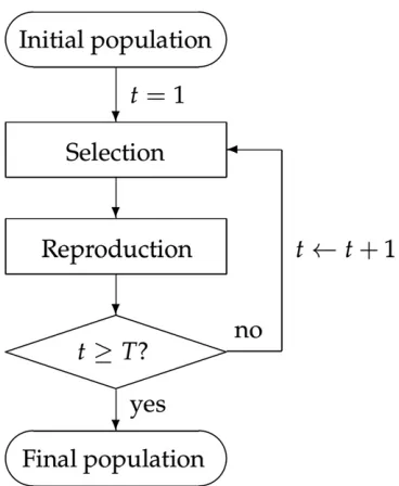
In silico breeding process model:The generic plant breeding
program considered in this paper is illustrated in Figure 1. Starting with an initial population, the program iterates over the selection, and reproduction steps ten times (T¼10) to simulate ten generations of breeding. In each simulation, 200 individuals were randomly selected from the 369 lines to form the initial population, and a breeding population of q¼20 individuals was selected in each generation. Each initial population was used once for all five selection approaches.
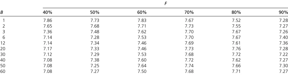
Five selection approaches were used in the selection step: GS, WGS, OHV, OPV, and GB. To determine appropri-ate parameter setting for the latter three approaches, 100 replicates of the generic plant breeding process were performed using 60 different combinations of the parameters: B2 f1;2;3;6;12;20;30;40;50;60g and F2 f40%;50%;60%;70%;80%;90%g For these three ap-proaches, the best combinations (B¼12; F¼70% for OHV; B¼60; F¼80% for GB; and B¼1; F¼40% for OPV) were used in 2000 additional simulation replicates of allfive approaches. Due to the large dimension of the data, the heuristic algorithm was used for OPV and GB in all simulations.
In the reproduction step, we use the following two substeps to simulate the next generation.
Substep 1: Pair the 20 selected individuals to make 10 crosses in descending order of their GEBVs, i.e., the individual with the highest GEBV is crossed with the sec-ond, the third highest with the fourth, etc.
Substep 2: Produce 20 progeny from each of the 10 crosses to maintain a population size of 200. Let r denote the vector of recombination frequencies and P2 f0;1gL32 the genotype matrix of a random offspring from crossing individualsn1 andn2:ThenPis determined as
Pi;j¼Ai;Jj
iþ1;nj;"i2 f1;. . .;Lg;j2 f1;2g:
Here, J1;J22 f0;1gL32
are two identical and independent random vectors following the inheritance distribution with recombination frequency vector r. The inheritance distribution was defined in Hanet al.(2017) as follows. Definition 0.1: Hanet al. (2017) We say that a random bi-nary vectorJ2 f0;1gLfollows aninheritance distribution with parameter vectorr2 ½0;0:5L21 if
J1¼
0; w:p: 0:5
1; w:p: 0:5; (13)
Ji¼
Ji21 w:p: 12ri21
12Ji21 w:p: ri21;"i2 f2;. . .;Lg: (14)
Here, “w.p.”stands for“with probability.”
This process was implementedin silicoin Octave (Eatonet al. 2015).
Results
Each selection approach was used in 2000 independent sim-ulation runs. Since each random initial popsim-ulation was used on allfive selection methods, the rankings of their population maximums in the 10th generations reveal their comparative effectiveness. Table 1 summarizes the frequencies of these rankings across the 2000 replications. These results suggest that OPV outperformed the other four approaches in achiev-ing genetic gains in thefirst 10 generations.
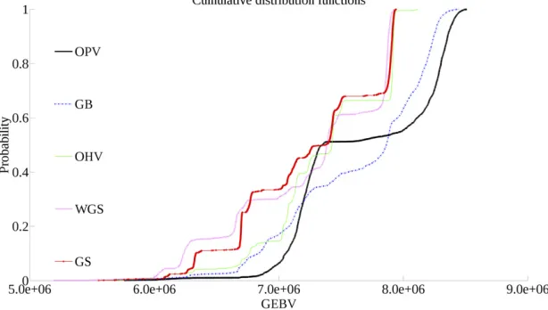
To provide a more insightful assessment of different selec-tion approaches, we also compared the cumulative distribu-tion funcdistribu-tions (CDFs) of the populadistribu-tion maximums in the 10th generation from each replicate (Figure 2). Since the vertical value of a point on a CDF curve indicates the percentage of random outcomes that have a lower GEBV than its horizontal value, the best performing selection approach at a given ver-tical point will be the farthest right. GS and WGS perform Figure 1 Diagram of the simulation process.
Table 1 Frequencies of relative rankings of the five selection approaches on the population maximum in the 10th generation across 2000 replications
GS (%) WGS (%) OHV (%) GB (%) OPV (%)
First 1.5 6.3 4.6 22.1 65.7
Second 11.6 6.4 27.6 46.8 7.7
Third 31.5 13.5 39.9 7.7 7.5
Fourth 33.9 19.5 25.5 14.1 7.2
similarly, although GS outperforms WGS below the 30th per-centile. Above the 40th percentile, OHV performs similarly to GS and WGS. Below this percentile, however, OHV out-performs both of these methods, matching the performance of GB. OPV outperforms GB below the 30th percentile and above the 50th percentile.
Figure 3 displays the means of population minimum, mean, and maximum of GEBV over 10 generations for all selection approaches. As expected, GS and WGS show quick and substantial improvement in GEBV before reaching a plateau at generation 4. OHV sacrifices short-term gain for long-term gain, exceeding the performance of GS and WGS by generation 9, 8, and 6 with respect to mean population minimum, mean, and maximum, respectively. GB demonstrates a similar growth pattern as OHV, with en-hanced performance across all three criteria. OPV has the slowest increases in mean population minimum; its mean population mean grows slowly in the firstfive generations butfinishes second to GB in generation 10; its mean popula-tion maximum initially improves more slowly than GS and WGS but eventually surpasses all other four approaches in generation 10.
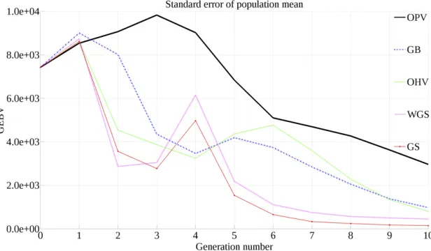
Figure 4 displays the SE of population mean over 10 gen-erations for all selection approaches. As expected, OHV, GB,
and OPV maintain genetic variance in the breeding popula-tion longer than either GS or WGS. However, OPV maintains substantially more genetic variance than either GB or OHV, indicating that there is greater room for population improve-ment after 10 generations.
Discussion
In this study, we have introduced a new selection approach, optimal population value selection (OPV), which evaluates the genetic merit of a set of selection candidates instead of performing truncation selection on an individual metric. OPV is similar to optimal haploid value (OHV) and genotype building (GB) in that all three methods consider the effects of recombination on the genetic merit of future individuals. By focusing on the GEBV of segments of the genome instead of total GEBV, these three methods can identify and select for segments that contain rare favorable alleles but whose favor-able effects would be discarded by truncation methods such as GS and WGS.
In our simulations, the primary advantage of OHV over GS and WGS is the decreased incidence of individuals with low GEBVs. The mean best individual over 10 generations is significantly better than the same individual from GS and Figure 2 Cumulative distribution functions of popula-tion maximums after 10 generapopula-tions of selecpopula-tion over 2000 replications for each selection approach.
WGS on average, although Figure 2 shows that there are rare cases where GS and WGS can match the performance of OHV. Daetwyleret al.(2015) reported that OHV maintained genetic variance longer than GS and hypothesized that this was due to the ability of OHV to maintain rare alleles in the population. OPV is similar to OHV with one important differ-ence. After calculation of optimal haploid values, OHV selection selects a fraction of individuals with the highest OHVs—a form of truncation selection. OPV selects a subset of individuals based on the maximum haploid value at individual segments across the selected individuals. Thus, there is still the possibility that OHV will discard individuals with rare favorable alleles that are masked by a large number of unfavorable alleles. OPV allows for the inclusion of individuals that have low genetic merit but contain favorable alleles that are rare in the rest of the selected individuals.
There are three principal differences between our imple-mentation of OHV and that of Daetwyleret al.(2015). First, the population sizes used in our study (200) are much smaller than those of Daetwyler et al. (2015) (55,000). One of the benefits of both OPV and OHV is their ability to maintain rare favorable alleles in breeding populations. Their ability to identify alleles is independent of population size, which increases the probability of obtaining favorable recombinants. Changes in population size are expected to affect both methods equally. Second, we have not imple-mented the use of DHs in our simulated breeding program as in Daetwyleret al.(2015). Despite this omission, we ob-serve that OHV outperforms GS. While a comparison of OPV and OHV when using DHs would be valuable, our results suggest that the advantage of OHV over GS is maintained without the use of DHs. Third, we removeF3100% of indi-viduals with the lowest GEBVs prior to selection, which is a strategy that has been shown to enhance the efficiency of OHV, OPV, and GB.
OPV is similar to GB, but it makes two improvements. First, the OPV metric exclusively measures the long-term potential of the most outstanding progeny in the population, whereas the GB metric also values the GEBV of the breeding parents like
GS does. Second, we presented an integer programming model and a heuristic algorithm for selecting an optimal subset of individuals to maximize the OPV or GB metric, which is an improvement over the algorithm presented in Kemper
et al.(2012). As Figure 3 shows, OPV and GB produce similar
response curves for the average of the best individuals. How-ever, when we consider the distributions of these best indi-viduals, we see that the worst of the best individuals produced by OPV are better than those of GB, and the best of the best individuals produced by OPV are better than those of GB. GB only outperforms OPV between the 30th and 50th percentiles. This indicates that while there is a chance that GB produces better individuals than OPV, in the best and worst cases, OPV is expected to be the superior method. One pos-sible explanation for this phenomenon is that OPV maintains genetic variance longer than all other methods (Figure 4).
Conclusions
In this paper, a new selection method, optimal population value (OPV) selection, was presented. Instead of using eval-uations of individual lines to select the breeding population, a candidate breeding population was selected as a unit. While this presents some computational challenges, such as solving a combinatorial optimization problem, it was shown to out-perform existing methods in a series of simulation experi-ments that spanned 10 generations, and used empirical data from an inbred maize population. Future research into geno-mic selection approaches should focus on selecting sets of individuals as a unit, rather than how to better evaluate individual breeding values prior to performing truncation selection.
Acknowledgments
This work was supported in part by the National Science Foundation grant IOS-1238142, the United States Depart-ment of Agriculture National Institute of Food and Agricul-ture (NIFA) Award 2017-67007-26175, and the Plant Sciences Institute at Iowa State University.
Literature Cited
Bernardo, R., and J. Yu, 2007 Prospects for genomewide selection for quantitative traits in maize. Crop Sci. 47: 1082–1090. Browning, B., and S. Browning, 2008 A unified approach to genotype
imputation and haplotype-phase inference for large data sets of trios and unrelated individuals. Am. J. Hum. Genet. 84: 210–223. Cole, J., and P. VanRaden, 2011 Use of haplotypes to estimate Mendelian sampling effects and selection limits. J. Anim. Breed. Genet. 128: 446–455.
Daetwyler, H., M. Hayden, G. Spangenberg, and B. Hayes, 2015 Selection on optimal haploid value increases genetic gain and preserves more genetic diversity relative to genomic selection. Genetics 200: 1341–1348.
Eaton, J. W., D. Bateman, S. Hauberg, and R. Wehbring, 2015 GNU Octave version 4.0.0 manual: a high-level interactive language for numerical computations. Available at: http://www. gnu.org/software/octave/doc/interpreter. Accessed: June 13, 2017. Fernando, R., and D. Garrick, 2009 Gensel—user manual for a portfolio of genomic selection related analyses. Technical report. Available at: http://bigs.ansci.iastate.edu/bigsgui. Accessed: June 13, 2017.
Goddard, M., 2009 Genomic selection: prediction of accuracy and maximisation of long term response. Genetica 136: 245–257.
Han, Y., J. Cameron, L. Wang, and W. Beavis, 2017 The predicted cross value for genetic introgression of multiple alleles. Genetics 205: 1409–1423.
Heffner, E. L., A. J. Lorenz, J.-L. Jannink, and M. E. Sorrells, 2010 Plant breeding with genomic selection: gain per unit time and cost. Crop Sci. 50: 1681–1690.
Jannink, J.-L., 2010 Dynamics of long-term genomic selection. Genet. Sel. Evol. 42: 1–11.
Kemper, K. E., P. J. Bowman, J. E. Pryce, B. J. Hayes, and M. Goddard, 2012 Long-term selection strategies for complex traits using high-density genetic markers. J. Dairy Sci. 95: 4646–4656. Leiboff, S., X. Li, H.-C. Hu, N. Todt, J. Yanget al., 2015 Genetic
control of morphometric diversity in the maize shoot apical meristem. Nat. Commun. 6: 1–10.
Meuwissen, T., B. Hayes, and M. Goddard, 2001 Prediction of total genetic value using genome-wide dense marker maps. Ge-netics 157: 1819–1829.
Schnable, P., S. Liu, and W. Wu, 2013 Genotyping by next-generation sequencing. U.S. Patent Application No. 13/739,874. Yu, J., J. Holland, M. McMullen, and E. Buckler, 2008 Genetic design and statistical power of nested association mapping in maize. Genetics 178: 539–551.
Appendix
Mean of maximal GEBV in the 10th generation for 100 random simulations using OHV (Table A1), GB (Table A2), and OPV (Table A3) selection. Optimal parameters are highlighted.
Table A1 Mean of maximal GEBV in the 10th generation for 100 random simulations using OHV selection
F
B 40% 50% 60% 70% 80% 90%
1 7.30 7.20 7.21 7.24 7.19 7.28
2 7.23 7.15 7.14 7.22 7.22 7.28
3 7.24 7.34 7.43 7.43 7.45 7.26
6 7.23 7.26 7.46 7.46 7.42 7.37
12 7.34 7.36 7.38 7.50 7.40 7.35
20 7.33 7.33 7.41 7.39 7.47 7.31
30 7.27 7.32 7.36 7.44 7.45 7.25
40 7.27 7.39 7.39 7.40 7.43 7.28
50 7.28 7.29 7.39 7.41 7.41 7.31
60 7.31 7.30 7.39 7.41 7.49 7.26
Table A2 Mean of maximal GEBV in the 10th generation for 100 random simulations using GB selection
F
B 40% 50% 60% 70% 80% 90%
1 7.71 7.69 7.69 7.70 7.57 7.27
2 7.26 7.50 7.53 7.46 7.47 7.30
3 7.33 7.45 7.50 7.67 7.64 7.28
6 7.25 7.37 7.52 7.65 7.76 7.42
12 7.18 7.39 7.56 7.71 7.71 7.34
20 7.15 7.35 7.54 7.70 7.73 7.30
30 7.19 7.29 7.61 7.73 7.72 7.20
40 7.12 7.34 7.59 7.68 7.70 7.31
50 7.10 7.29 7.55 7.67 7.64 7.27
60 7.17 7.22 7.64 7.74 7.77 7.26
Table A3 Mean of maximal GEBV in the 10th generation for 100 random simulations using OPV selection
F
B 40% 50% 60% 70% 80% 90%
1 7.86 7.73 7.83 7.67 7.52 7.28
2 7.65 7.68 7.71 7.73 7.55 7.27
3 7.36 7.48 7.62 7.70 7.67 7.26
6 7.14 7.28 7.53 7.70 7.67 7.40
12 7.14 7.34 7.46 7.69 7.61 7.36
20 7.17 7.33 7.46 7.73 7.76 7.28
30 7.12 7.29 7.53 7.68 7.72 7.22
40 7.08 7.38 7.60 7.72 7.62 7.27
50 7.08 7.25 7.64 7.74 7.66 7.30