ABSTRACT
A HIGH PERFORMANCE COMPUTER MODEL FOR SOUND PROPAGATION IN THE HUMAN THORAX
By
CHANDRASEGARAN NARASIMHAN
A thesis submitted to the Graduate Faculty of North Carolina State University
in partial fulfillment of the requirements for the Degree of
Master of Science
CIVIL ENGINEERING
Raleigh
2001
APPROVED BY:
________________________________
BIOGRAPHY
ACKNOWLEDGEMENT
This project was partly funded by Oak Ridge National Laboratory (ORNL) through Laboratory Directed Research and Development (LDRD) funds. I thank the Computer Science & Mathematics directorate at ORNL for letting me use the IBM SP-2 throughout the project. I thank National Library of Medicine for providing the visible human data set.
TABLE OF CONTENTS
Page
LIST OF FIGURES vi
1. INTRODUCTION 1
1.1 The Virtual Human 1
1.2 The Motivation 2
1.3 Literature Review 2
1.4 Objective 4
1.5 Assumptions in the model 4
2. MATHEMATIC MODELS AND NUMERIC APPROXIMATIONS 6
2.1 Governing Equation 6
2.2 CT Data 7
2.3 Initial and Boundary conditions 8
2.4 Justification for reflecting boundary condition 9
2.5 Initial pulse problem 9
2.6 Driving function problem 10 2.7 Finite Difference Approximation 11 2.8 Criterion for Stability 13
3. PARALLEL IMPLEMENTATION 16 3.1 Parallelization 16
3.2 Interpolation 19 3.3 CT data distribution 20 3.4 Parallel IO and restart option 20
4. RESULTS AND CONCLUSIONS 22 4.1 Comparison of Numerical Schemes 23 4.2 Effect of driving frequency 24
4.3 Effect of sampling point 26
4.4 Effect of CT data resolution 29 4.5 Effect of size of Human Thorax 31 4.6 Constant density simulation 32
4.7 Initial pulse problem 33
4.8 Performance Evaluation 34
4.9 Conclusions 36
LIST OF FIGURES
LIST OF FIGURES Page MATHEMATIC MODELS AND NUMERIC APPROXIMATIONS
2.1: An example CT image and the corresponding density image. 8 2.2: CT density image with regions with air density in blue. 9
2.3: Sound wave front and grid front 14
PARALLEL IMPLEMENTATION
3.1: Diagram showing domain decomposition 17
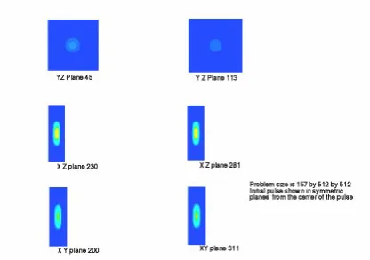
3.2: Schematic diagram showing 7-point and 13-point schemes 18 3.3: Diagram showing ghost region consisting of two planes 18 3.4: Diagram showing exchange of data between ghost regions 19 3.5: Initial pulse in three different planes 21 RESULTS AND CONCLUSIONS
4.1: CT image with the four sample points 23 4.2: Solution obtained from Equations 2.7 and 2.8 24 4.3: Time series plots for different driving frequencies 25
4.4: Power Spectrum plots for different driving frequencies 27
4.5: Enlarged Power Spectrum plots 28
4.6: Time series plots based on a single driving frequency 29 4.7: Power spectrum for readings at various sampling point 30 4.8: Power spectrum for runs with different data resolution 31 4.9: Time series plot for “small thorax” simulation 32 4.10: Time series and Spectrum plots from constant density simulation 33 4.11: Time series and power spectrum for initial pulse problem 34
Chapter 1
Introduction
Computers have long been used for modeling physical systems that are difficult or impossible to model experimentally. This is particularly true for human systems because employing human subjects for studying a given scenario is not always possible due physical, ethical and financial reasons. However, computer modeling of human systems is a challenging task because these systems are incredibly complex (three dimensional problems with complex fluid flow, elastic and moving tissues, heterogeneous composition etc.). With the emergence of parallel supercompters in the recent years, modeling complex systems such as the human body is becoming increasingly feasible. However, if we are to take advantage of these modern computing environments for human system modeling, new algorithms and models that can effectively simulate these systems need to be developed. This thesis is a small step towards this goal with a focus on pulmonary acoustics. Modeling acoustic signatures in the respiratory system based on auscultation is a very important area in pulmonary diagnostics. An overall objective of this thesis is to develop a high-resolution supercomputer model for sound propagation in the human thorax based on realistic tissue data and analyze how sound is propagated through this region of the body.
1.1 The Virtual Human
(ORNL) recently embarked on an initiative called “The Virtual Human” that seeks to develop a functional computer model of the human body and has the potential to become the perfect, non-invasive tool for monitoring and diagnosing patients. But to make these ambitious goals a reality, each individual sub-system has to be modeled, tested and incorporated into The Virtual Human separately. The work described in this thesis is an attempt toward a very small component of the overall Virtual Human, namely the sound propagation in the pulmonary system.
1.2 The Motivation
With exponential increase in computing power and advances in computational algorithms, a lot of attention has been focused on the spectral analysis of breath sounds, CFD of airflow through lung airways, and computational biomechanics of lung tissues. Despite the fact that we have a greater understanding regarding breath sounds, several questions remain unanswered. For example, where are the predominant regions in the lung airways where the sounds are generated? What role does movement of lung tissues and air wall vibrations play in the generated sounds? What range of sound frequencies are propagated to different chest wall locations? Answers to these questions are very critical in clinical respiratory physiology where initial diagnosis is often based on auscultation.
The importance of accurately accounting for all the sources of lung sounds is best illustrated by a quote from Olson and Hammersely (1985): “Understanding the detailed relationship between airflow and sound genesis, and airway wall elasticity to sound production and modification, may permit the development of a powerful noninvasive tool for evaluating ventilatory function and the anatomic status of airway”. An accurate virtual model of pulmonary sub-system cannot only help answer various unanswered questions but also achieve the goal of being non-invasive.
1.3 Literature Review
consequently developing better diagnostic procedures. As the air flows through the lung it generates sound and this sound propagates to the rest of the body. While it is known that mechanisms such as air wall vibrations and fluid film rupture contribute to
adventitious sounds (breath sounds of people who are sick) such as wheezing, it is not
clear whether these factors and other factors such as lung tissue movement play a role in the generation of normal breathing sounds [Macklem 1996]. Recent advances in computing technology have significantly improved our understanding of lung sound generation and propagation mechanisms [Pastercamp et al., 1997]. In particular, we now have the algorithms and computing power to perform detailed spectral analyses of recorded and observed sounds [Allgood et al. 2000, Kraman et al. 1998, Wodicka et al., 1994]. These analyses have given us a deeper understanding of predominant sound frequencies generated by different mechanisms. For example, empirical techniques such as artificial neural networks can be used to correlate lung obstructions and recorded breath sounds. Such correlations can be used for predicting potential lung obstruction locations from recorded breath sounds.
Numerous experiments have been performed to study sound propagation through the lung parenchyma and the relationship to phase delays and frequency spectrums of the observed sounds at various chest wall locations. Phase delay experiments using He-O2 conducted by Patel et al. (1995) indicated that the higher frequency components take more of an airway borne route (the lung airway acts as a wave guide) while the lower frequency components propagate through the surrounding lung parenchyma. Related experiments performed by Lu et al., 1995 confirmed that sound at higher frequencies reach the chest wall faster than that at lower frequencies.
was a simple domain because the simulation was confined to the skull of the dolphin and there were not lot of density variations.
1.4 Objectives
Modeling the pulmonary system can be broken down into two sub-problems. The first part is the sound generation, where one solves the Navier Stokes equation for airflow in the lung and the second part is the propagation, where one solves the wave equation for heterogeneous medium. The objective of this project is to develop a simulation code for a sound propagation model in human body.
The objectives of this project are
• To model sound propagation by taking into account the various physical features of the human body more accurately by using CT scan images from the visible human male data set (See CT image in Chapter 2).
• To Parallelize the model to enable high-resolution simulations on modern supercomputers.
• To study the effects of various factors like spatial inhomogeneity, size of the chest, confinement of sound waves in chest and frequency of the source on sound recorded and to do a spectral analysis of the same.
The pressure output from the sound generation part becomes the input for sound propagation part and hence can be combined into a single code. A working code for sound generation is yet to be developed. When complete, sound generation code, along with the sound propagation code, will help model human breath sounds.
1.5 Assumptions in the model
The following assumptions are made in developing a mathematical model for sound propagation.
• Medium behaves like a fluid
Future work can adopt a more complicated model by treating the human thorax as an elastic medium with properties like Young’s modulus, etc. One might have to do an extensive literature review or perform experiments to come up with various parameters required for an elastic model.
• Dynamic effects of medium are ignored
The CT data is not time varying even though when we breathe the chest expands and contracts as well as blood flows into and out of the heart. So one cannot take into account the dynamic effects of density variation in sound propagation simulation.
• Reflective boundary condition on upper and lower thorax
Sound waves do not pass through the diaphragm located below the lung to the rest of the lower body. Sound waves neither pass through the shoulders to the arms nor to the head through the neck. In other words sound waves are confined to the chest region (the thorax). Hence an internally reflecting boundary condition has been implemented.
Some of the above assumptions are likely to have an effect on the solution generated. But this is the first attempt in modeling sound propagation for accurate representation of major features of the human body. Future work can improve on the current model, and better assumptions can be made which are close to real pulmonary systems.
Chapter 2
Mathematic Models and Numeric Approximations
This chapter presents the mathematical framework for developing the sound propagation model. The basic mathematical equations and the boundary conditions are described. The various numerical schemes considered along with the stability condition have also been elaborated.
2.1 Governing Equation
For sound propagation in a heterogeneous medium the governing partial differential equation is of the form [Aroyan 1996]
2
2
2 2
1 ( , ) ( , ) ( )
( , )
( ) ( )
P t P t
P t c t ρ ρ ∂ − ∇ = −∇ ∇ ∂
x x x
x
x x
g
(2.1) Where P is the acoustic pressure, ρ is tissue density and c is its corresponding
speed of sound. The right hand side of the equation takes into account the variation in density of the medium. Another equivalent mathematical form of equation 2.1 is [Aroyan 1992]
2
2 2
1 ( , ) 1
( ) ( , )
( ) ( )
P t
P t
c t ρ ρ
∂ = ∇ ∇ ∂ x x x
x g x (2.2)
For a simple homogeneous medium both equations 2.1 and 2.2 reduces to 2
2
2 2
1 ( , )
( , ) P t P t c t ∂ = ∇ ∂ x
2.2 CT Data
One of the major differences between the current approach and previous studies pertaining to sound propagation in the human lung is the use of Computed Tomography (CT) scan data. Equations 2.1 and 2.2 require the density of human thorax and velocity of sound at various points in the human thorax for calculating acoustic pressure. CT data is used to obtain an exact representation of human body features. The Visible Human is an anatomical data set developed under a contract from the National Library of Medicine by the Departments of Cellular and Structural Biology, and Radiology, University of Colorado School of Medicine. CT values from the Visible Human male CT images are used to obtain the density of corresponding tissue [Aroyan 1996]. The velocity, the only other parameter required, can be obtained from the corresponding tissue density [Aroyan 1996]. The following empirical relationships (obtained from the unpublished work of a student of Dr. Richard Ward at ORNL) were used to get density and velocity.
-5 3 7 2 11 3
6
(g/cc) 1×10 +1.24 10 -2.83 10 2.79 10
(mm/sec)=( 0.112) 1.38 10
r r r
c
ρ
ρ
− − −
= × × + ×
+ × ×
where r is the CT value.
Figure 2.1: An example CT image and the corresponding density image.
2.3 Initial and Boundary conditions
Figure 2.2: CT density image with regions with air density in blue.
2.4 Justification for reflecting boundary condition
Flesh has the same density as that of water and hence the boundary condition used for air water interface can also be used for air-flesh interface. The pressure amplitude reflection coefficient water air, for normally incident sound wave is given by
, 0.9994
air water
water air
air water
Z Z
Z Z
−
= =
+
as
0.0003
air air water water
air
water
c Z
Z c
ρ ρ
= =
In the case of constant frequency the ratio of energy per unit area per unit time reflected to that of incident is given by
, 2 Energy reflected
0.9988
Energy incident =water air = (2.4)
Thus there is an error of 0.12% because of a totally reflecting boundary condition assumption.
complex source is broken down to some specific frequencies. The initial pulse problem has a pressure distribution at time t=0 and this distribution is propagated and studied with respect to time. The initial pulse chosen is a spatial sin square function contained within 1/10 the length of the domain in all three directions. Thus the initial and boundary conditions become
Initial Conditions:
2 2 2
( , 0) cos cos cos
2 2 2 2 2 2
y
x z
x y z
l
l l
P t x π y π z π
ε ε ε = = − − − x if 2 2 i i
i i i
l l
x
ε ε
− < < +
0
= if or
2 2
i i
i i i i
l l
x < −ε x > +ε
where and , ,
20
i i
l
i x y z
ε = = 0 ( , ) 0 t P t t = ∂ = ∂ x
for all x
Boundary Conditions:
P( , )x t =0 if ρ( )x <0.1g/cc
Simulation results are presented in chapter 4.
2.6 Driving function problem
In the driving function problem a single frequency is used to drive the system throughout the simulation. Thus one can analyze the behavior of the medium for a specific frequency.
Initial Conditions:
( , 0) 0
P x t= = for all x
0 ( , ) 0 t P t t = ∂ = ∂ x
Boundary Conditions:
P a b c t( , , , )=sin(2π ft)
P( , )x t =0 if ρ( )x <0.1g/cc
Here (a,b,c) is a location in human thorax and f is the driving frequency.
2.7 Finite Difference Approximation
Two different FD schemes were implemented. The first scheme developed was Aroyen’s scheme [Aroyan 1996] with the incorporation of terms for anisotropy. This scheme was developed from equation 2.1 and is fourth order in space for pressure, second order in space for density and second order in time derivative of pressure (equation 2.5).
( )
(
)
(
)
(
)
1 2 2 2 2 2 1
, , , , , , , , , , , ,
2 , ,
2 2
1, , 1, , , 1, , 1, , , 1 , , 1
2 , ,
2 2, , 2, ,
2 2.5 2.5( / ) 2.5( / )
4 / 3
1/ ( ) 1/ ( )
(1/12)
1/ (
t t t
i j k i j k i j k i j k i j k i j k
i j k
t t t t t t
i j k i j k i j k i j k i j k i j k
i j k
t t
i j k i j k
P P P
P P P P P P
P P κ κ α κ β κ α β κ α + − + − + − + − + − = − − − − + + + + + + −
+ +
(
2)
, 2, , 2, , , 2 , , 2 2
, ,
1, , 1, , 2, , 2, , 1, , 1, , , ,
2 2
, , , 1, , 1, , 2,
) 1/ ( )
(1/ 3)
( ) (1/ 8)( )
( ) /
(1/ 3)( / ) ( ) (1/ 8)(
t t t t
i j k i j k i j k i j k
i j k
t t t t
i j k i j k i j k i j k
i j k i j k i j k
t t t
i j k i j k i j k i j k
P P P P
P P P P
P P P
β κ ρ ρ ρ κ α + − + − + − + − + − + − + + + + − − − − −
− − − , 2,
, 1, , 1, , ,
2 2
, , , , 1 , , 1 , , 2 , , 2 , , 1 , , 1 , ,
)
( ) /
(1/ 3)( / ) ( ) (1/ 8)( )
( ) / (2.5)
t
i j k
i j k i j k i j k
t t t t
i j k i j k i j k i j k i j k
i j k i j k i j k
P
P P P P
ρ ρ ρ κ β ρ ρ ρ − + − + − + − + − − − − − − − −
( )
(
)
(
)
(
)
1 2 2 2 2 2 1
, , , , , , , , , , , ,
2 , ,
2 2
1, , 1, , , 1, , 1, , , 1 , , 1
2 , ,
2 2, , 2, ,
2 2.5 2.5( / ) 2.5( / )
4 / 3
1/ ( ) 1/ ( )
(1/12)
1/ (
t t t
i j k i j k i j k i j k i j k i j k
i j k
t t t t t t
i j k i j k i j k i j k i j k i j k
i j k
t t
i j k i j k
P P P
P P P P P P
P P κ κ α κ β κ α β κ α + − + − + − + − + − = − − − − + + + + + + −
+ +
(
2)
, 2, , 2, , , 2 , , 2 2
, ,
1, , 1, , 2, , 2, ,
, , 1, , 1, , 2, , 2, ,
2 2
, , , 1,
) 1/ ( )
(4 / 9)
( ) (1/ 8)( )
(1/ ) ( ) (1/ 8)( )
(4 / 9)( / ) (
t t t t
i j k i j k i j k i j k
i j k
t t t t
i j k i j k i j k i j k
i j k i j k i j k i j k i j k
i j k i j k
P P P P
P P P P
P β κ ρ ρ ρ ρ ρ κ α + − + − + − + − + − + − + + + + − − − − − − −
− , 1, , 2, , 2,
, , , 1, , 1, , 2, , 2,
2 2
, , , , 1 , , 1 , , 2 , , 2 , , , , 1 , , 1
) (1/ 8)( )
(1/ ) ( ) (1/ 8)( )
(4 / 9)( / ) ( ) (1/ 8)( )
(1/ ) ( )
t t t t
i j k i j k i j k
i j k i j k i j k i j k i j k
t t t t
i j k i j k i j k i j k i j k
i j k i j k i j k
P P P
P P P P
ρ ρ ρ ρ ρ κ β ρ ρ ρ − + − + − + − + − + − + − − − − − − − − − − −
− (1/ 8)(ρi j k, , +2 ρi j k, , −2) (2.6)
− −
Yet another scheme can be obtained from equation 2.2. This scheme is second order in both space and time for both density and pressure and uses central difference. See equation 2.7.
2
, , , , 2, , , , , , 2, ,
1 1
, , , , , ,
1, , 1, ,
2
, , , , , 2, , , , , , 2, 2
, 1,
2
4
4
t t t t
i j k i j k i j k i j k i j k i j k
t t t
i j k i j k i j k
i j k i j k
t t t
i j k i j k i j k i j k i j k i j
i j k
P P P P
P P P
P P P P
κ ρ ρ ρ κ ρ α ρ + − + − + − + − + − − = − + − − − + −
, 1,
2
, , , , , , 2 , , , , , , 2 2
, , 1 , , 1
(2.7) 4
t k
i j k
t t t t
i j k i j k i j k i j k i j k i j k
i j k i j k
P P P P
ρ κ ρ β ρ ρ − + − + − − − + −
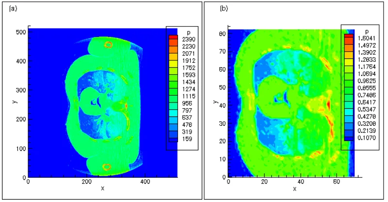
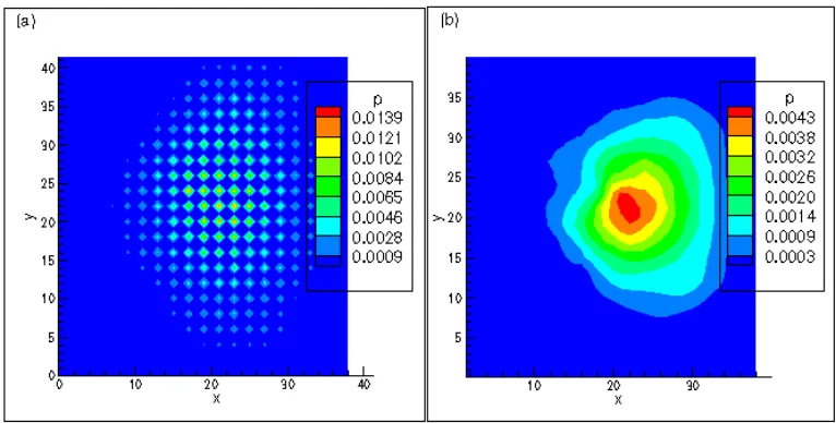
The above scheme had the drawback of propagating the sound to alternate grid points for a point source (see results in next chapter). So a new scheme was developed (equation 2.8) which makes use of forward and backward difference for calculating pressure gradient.
2
, , , , 1, , , , , , 1, ,
1 1
, , , , , ,
1, , 1, ,
2
, , , , , 1, , , , , , 1, 2
, 1,
2
2
2
t t t t
i j k i j k i j k i j k i j k i j k
t t t
i j k i j k i j k
i j k i j k
t t t
i j k i j k i j k i j k i j k i j
i j k
P P P P
P P P
P P P P
κ ρ ρ ρ κ ρ α ρ + − + − + − + − + − − = − + − − − + −
, 1,
2
, , , , , , 1 , , , , , , 1 2
, , 1 , , 1
(2.8) 2
t k
i j k
t t t t
i j k i j k i j k i j k i j k i j k
i j k i j k
P P P P
ρ κ ρ β ρ ρ − + − + − − − + −
Equations 2.6 and 2.7 have an extra boundary condition that P( , )x t =0 if 1, 1, 1 0
i j k
ρ± ± ± = i.e. none of the neighboring points can’t have density of 0 because they appear in the denominator of both equations. A comparison of all these schemes is discussed in chapter 4.
2.8 Criterion for Stability
For the 1 Dimensional wave equation in a homogeneous media the criteria for stability is given by equation [Hoffman 1992]
max
x t
c
∆
∆ <= (2.9)
Figure 2.3: Sound wave front represented as a circle and grid front shown as a rhombus
This limitation is explained with the following 2D example. At any time t wave front from sound source forms of a circle where as the ‘computational front’ from a source forms a rhombus. See figure 2.3. Whole of the wave front should be contained in the computational front. Thus the circle should be contained within the rhombus.
max
max 1
OC OB OA
2 1
2 1
2
n c t n x
x t
c <= =
× × ∆ <= × ∆
∆ ∆ <=
For the Three Dimensional homogeneous isotropic wave equation, the stability criterion becomes
A B
O
xy
C
max
1
3 x t
c
∆
∆ <= (2.10)
Chapter 3
Parallel Implementation
This chapter deals with the basic methodology used in implementing the FDM for the PDE in a parallel environment along with a host of other issues. This chapter is also written with an intention to help potential future users of the code.
3.1 Parallelization
The motivation to implement the algorithm in a parallel environment was two fold. First, the small grid spacing desired to resolve the fine features of the CT data resulted in very high memory requirements. Second, the explicit scheme adopted required very small time steps thus placing a very high premium on computation speed. Parallelization can alleviate both of these difficulties. Since linear interpolation was to be implemented to handle any instability that might arise due to density variations, the memory constraint was considered to be a real hurdle.
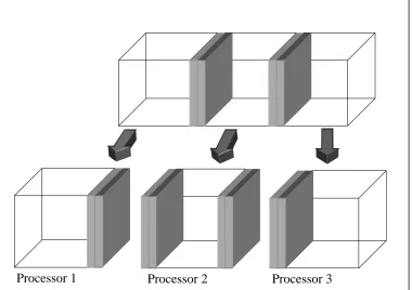
The algorithm adopted for parallelizing the explicit FDM is a one dimensional domain decomposition technique. Domain decomposition is an approach in which the whole computation domain is divided into smaller sub-domains. Computation on every sub-domain is handled by a single processor [Gropp and Keyes 1988]. One dimensional domain decomposition refers to a case in which the planes of divisions are perpendicular to one of the orthogonal directions. See Figure 3.1. One dimensional domain decomposition was employed because they are easy to implement and it was more important to verify the numerical scheme.
Processor 1 Processor 2 Processor 3
on. The finite difference scheme being employed used either a 13-point or a 7-point stencil depending on whether the partial derivative was approximated to a forward differencing or central differencing scheme (Figure 3.2). For the 13-point scheme, the processor computing values at the edge of its domain must have values at two points from its neighboring processors domain, meaning that two planes constitute a ghost region. See Figure 3.3.
Figure 3.2: Schematic diagram showing 7-point and 13-point schemes
Figure 3.3: Diagram showing ghost region consisting of two planes
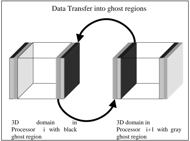
After every time step each processor gets data into its ghost region from its neighboring processor (in the context of adjacent sub domains and not physically adjacent processors). This data transfer can be done without any copying into a temporary buffer if the grid points are in consecutive locations in memory. See Figure 3.4.
Data transfers were accomplished by using the Message Passing Interface (MPI), a parallel library for inter processor communication [MPI: Message Passing Interface, Gropp et al. 1999a]. MPI works by sending and receiving messages (data packets) between processors. There are various ways of sending and receiving messages through MPI. There is simple MPI-send and MPI-receive, which first waits for communicating
Seven point Thirteen point
=
+
processors to establish communication, and then exchanges data. Another method is through use of persistent communication in which the latency due to establishment of communication between processors is avoided by predefining the buffers needed for transfer of data.
Figure 3.4: Diagram showing exchange of data between ghost region
3.2 Interpolation
Abrupt spatial changes in density can cause instability in some of the numerical schemes like equations 2.5 and 2.6. An interpolation approach was implemented to alleviate this problem. A simple tri-linear interpolation was first implemented in the serial code and then extended to the parallel code. At the macroscopic level the 3D CT data is visualized as stacks of cuboids with values known at the eight vertices. These cuboids can be divided into a series of planes and these planes can in turn be divided into series of lines. Thus with a function which does linear interpolation between two points in space 3D interpolation of CT data can be carried out. A series of cuboid interpolation routines
3D domain in Processor i with black ghost region
3D domain in
Processor i+1 with gray ghost region
Since there are 2 planes of ghost data, a separate linear interpolation has to be performed in the ghost regions of each processor. The processors will also be reading two more CT slices (one for positive x and one for negative x) even though they will not be computing pressure at the corresponding grid points. The extra CT slices are needed for interpolation in the ghost region. The interpolation has to proceed in the negative direction for the ghost regions at the beginning of the computation domain and in the positive direction at the end of computation domain.
The code will require at least one point interpolation in x direction because if no interpolation is performed then all the planes in the ghost region will have to be filled with actual CT images. Thus each processor has to read four images instead of two images.
3.3 CT data distribution
The CT scan of horizontal slices of human thorax exists as separate image files. For fast and efficient transfer of data between processors they need to be consecutive in memory. Thus it would be best to orient the CT slices along the plane of ghost regions. In this code CT data is oriented along the yz plane. By performing serial IO in parallel the CT data is distributed among various processors, i.e., each processor reads a set of CT data corresponding to its domain. When a 13-point stencil is being used, CT images of sub-domains in neighboring processors are required for computing pressure. Thus each processor also reads two extra CT slices, one corresponding to each side of the domain, for computing interpolated CT values in the ghost region.
3.4 Parallel IO and restart option
by the user. Hence the distributed domains in the memory of the processors can be mapped to the single continuous domain in the hard disk.
Chapter 4
Results and Conclusions
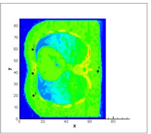
This chapter presents the spectral analysis of simulation results and parallel performance results. For all the simulations in this chapter, every fourth CT image in the range 1300 to 1508 was used. Since the images have a 1 mm spacing between them, a total body height of 208 mm was considered in the simulations. This range of images contains the regions from shoulder to diaphragm. The spacing between the data points in each plane was 4 mm for all the runs except for one, for which, the spacing was 8mm[G1]. One of the planes in this range is shown in the Figure 4.1. The figure shows the two lobes of the lung, the rib cage and the heart. The figure also shows four points at which pressure readings were recorded.
Figure 4.1 : CT image with the four sample points
4.1 Comparison of Numerical Schemes
Figure 4.2: Solution obtained from Equation s2.7 (figure (a)) and 2.8 (figure (b))
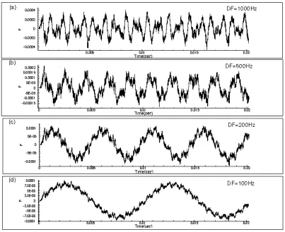
4.2 Effect of driving frequency
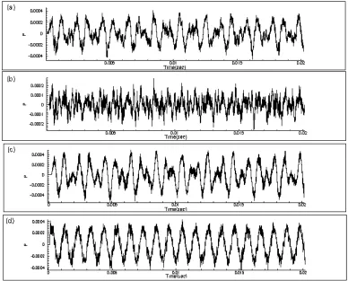
To study the behavior of sound propagation in human thorax, four separate runs with driving sinusoidal frequency (DF) values of 1000Hz, 500Hz, 200Hz and 100Hz were performed with CT data resolution of 4mm by 4mm by 4mm. Pressure readings from sample point 1 in Figure 4.1 were taken for all the runs for time series and spectral analysis.
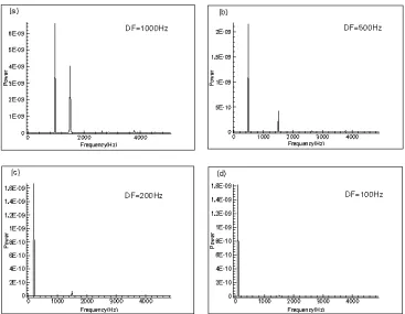
With respect to the analysis of breath sounds, it has been observed that very sensitive microphones are needed to pickup sounds of order 1000Hz [Pasterkamp et al. 1996]. If breath sounds mainly constitute of frequencies around 100Hz [Gavriely et al. 1981], from the power spectrum of figures 4.4(d) and 4.5(b), one can see that the power associated with frequencies around 1000Hz will be less. The model also validates the current practice of amplifying frequencies of around 100Hz in stethoscopes [Abella et al. 1981], as frequencies in that range are transmitted most effectively through the thorax.
Figure 4.3: Time series plots for different driving frequencies observed at sampling point 1. (a) DF=1000Hz, (b) DF=500Hz, (c) DF=200Hz, (d) DF=100Hz. Refer to figure 4.1 for location of sampling
4.3 Effect of sampling point
To observe the way sound propagates to different parts of the human thorax and to determine which frequencies are propagated effectively to different regions of the pneumo-thorax surface, four separate runs with a DF of 1000Hz were sampled for pressure at the four points in Figure 4.1. The CT data resolution was 4mm by 4mm by 4mm. DF of 1000Hz was chosen because its secondary peaks had higher power.
.
Figure 4.4 : Power Spectrum plots for different driving frequencies observed at sampling point 1. (a) DF=1000Hz, (b) DF=500Hz, (c) DF=200Hz, (d) DF=100Hz. Refer to figure 4.1 for location of sampling
Figure 4.6: Time series plots based on a single driving frequency of 1000 Hz observed at different sampling points. (a) sampling point 1, (b) sampling point 2, (c) sampling point 3, (d) sampling point 4. Refer to
figure 4.1 for location of each sampling point.
4.4 Effect of CT data resolution
Figure 4.8: Power spectrum for runs (a) with data resolution 8mm and (b) with resolution 4mm.
4.5 Effect of size of Human Thorax
Figure 4.9: Time series plot (plot (a)) and the corresponding power spectrum (plot (b)) for “small thorax” simulation
4.6 Constant density simulation
Figure 4.10: Time series and Spectrum plots from constant density simulation
4.7 Initial pulse problem
Figure 4.11: Time series (plot (a)) and power spectrum of time series (plot (b)) for initial pulse problem.
4.8 Performance Evaluation
speed switch between the nodes for inter processor communication. Standard performance evaluations show a latency of 24 microseconds and a bandwidth of 133Mb per second for MPI communications.
(a) Scalability
0 2000 4000 6000 8000 10000
0 20 40 60 80 100 120
Processors
Mf
lo
p Persistent
Simple
(b) Speed Up
0 25 50 75 100
0 20 40 60 80 100 120 Processors
Mf
lop pe
r Pr
oc
e
ss
o
r
Persistent Simple Send
Figure 4.12: Scalability (plot (a)) and speedup plots (plot (b))
simulation will be longer because higher resolution also means smaller time step because of smaller grid spacing. Higher resolution also mean larger data transfers between processors and hence, will lead to more communication latency. Thus the problem gets worse with more data points. Implementing three-dimensional domain decomposition can solve some of these problems. 3D domain decompositions generally have better scalability and lesser communication overhead (Kumar et al. 1994).
4.9 Conclusions
In spite of the various limitations and assumptions in the model, the sound propagation simulation reproduces certain characteristics observed in breath sounds. The model suggests that frequencies of the order of 100Hz are most effectively transmitted through the thorax and there seems to be a resonance effect at 1500Hz (secondary peak in the spectra). The results indicate that the way the sound propagates in the thorax can generate higher frequency sounds on the chest wall. The model also exhibits spatial inhomogeneity of sound propagation. A comparison of the spectrum from a homogeneous medium with that of human thorax suggests that the frequency of the second maxima in the spectrums are affected by the spatial confinement of the sound waves. The spectrum from the homogeneous simulation was also found to have very little features when compared to that of the one from thorax. This implies that the complex spectrum observed for a human thorax is probably due to the various features within the thorax like bones, lungs, hearts etc. The model confirms that the size of the thorax plays a significant role in the type of sound generated at the chest wall.
computation domain, might cause more sound to be propagated through the heart. In humans the sound source is located at the larger airways. The assumption that the sound waves are confined to the thorax may not be valid. It might be better to assume that a certain fraction of sound wave propagates to the lower parts of the body and hence never reenter the thoracic region. The periodic variations associated with density, volume, and tissue movements of the thorax have been ignored. Future work can be directed toward addressing these issues.
LIST OF REFERENCES
Abella, M., Formolo, J., and Penney, D.G. (1992). Comparison of the Acoustic Properties of six Popular Stethoscopes. J. Acoust. Soc. Am. 91:2224-2228.
Aroyan, J.L. (1996). Three-dimensional Numerical Simulation of Bisonar Signal Emission and Reception in the Common Dolphin. Ph.D. Dissertation. U.C. Santa Cruz, 1996.
Aroyan, J.L., T.W. Cranford, J. Kent, and K.S. Norris (1992). Computer modeling of acoustic beam formation in Delphinus delphis, J. Acoust. Soc. Am. 92(5), November 1992.
Gavriely, N., Palti, Y., and Alory, G. (1981). Spectral Charecteristic of Normal Breath Sounds. J. Appl. Physiol. 50:307-314.
Gropp W. D., and D.E. Keyes, Complexity of parallel implementation of domain decomposition techniques for elliptic partial differential equations., SIAM J. Sci. Stat. Comp. 9(2): 312-326. Mar 1988.
Gropp, W., Lusk E., and Skjellum A., (1999a). Using MPI: Portable Parallel Programming with the Message-Passing Interface. Second Edition, The MIT Press, Cambridge, MA.
Gropp, W., Lusk E., and Thakur R., (1999b). Using MPI-2: Advanced features of the Message-Passing Interface. First Edition, The MIT Press, Cambridge, MA.
Hoffman, J.D., (1992). Numerical Methods for Engineers and Scientists. Mc Graw Hill. Ihlenburg, F. (1998). Finite Element Analysis of Acoustic Scattering. Springer-Verlag, New York.
Kraman SS, Pasterkamp H., Kompis M., Takase M., Wodicka G.R., (1998). Effects Of Breathing Pathways On Tracheal Sound Spectral Features. Respiration Physiology. 111: (3) 295-300 MAR 1998.
Kumar V.P., A. Grama, A. Gupta, G. Karypis, (1994). Introduction to Parallel Computing: Design and Analysis of Algorithms, p. 597, Benjamin/Cummings Publishing Co., Ltd., Redwood City, CA.
Lu S., Doerschuk P.C., Wodicka G.R. (1995). Parametric Phase-Delay Estimation Of Sound Transmitted Through Intact Human Lung. Med. & Biol. Eng. &Comput. 33: (3) 293-298 May 1995.
Macklem, P.T., (1996). Invited Editorial on “Airflow effects on amplitude and spectral content of normal breath sounds”. Journal of Applied Physiology. 80(1), 3-4, 1996.
Mast, T.D., Hinkelman, L.M., Metlay, L.A., Orr, M.J., Waag, R.C. (1999). Simulation of Ultrasonic Pulse Propagation, Distortion, and Attenuation in the Human Chest Wall. J. Accoust. Soc. Am. 106(6): 3665-3677.
O’ Donnell, D.M., and Kraman, S.S. (1982). Vascular Lung Sound Amplitude Mapping by Automated flow-gated Phonopneumography. J. Appl. Physiol. 53:603-609.
Olson, D.E., and Hammersely, J.R., (1985). Mechanisms of Lung Sounds Generation. Seminars in Respiratory Medicine. 6(3), 171-179, 1985.
Pastercamp H., Kraman S.S., and Wodicka, G. R. (1997a). State of the Art: Respiratory Sounds - Advances Beyond the Stethoscope. American Journal of Respiratory Care Medicine. 156, 974-987, 1997.
Pastercamp H., Patel S., and Wodicka, G. R. (1997b). Asymmetry of Respiratory Sounds and Thoratic Transmision. Med. & Biol. Eng. &Comput. 35, 103-106, 1997.
Patel S., Lu S., Doerschuk P.C., and Wodicka G.R. (1995). Sonic Phase Delay From Trachea To Chest-Wall - Spatial And Inhaled Gas Dependency. Med. & Biol. Eng. &Comput. 33: (4) 571-574 Jul 1995.