High Speed Model Implementation and Inversion Techniques
for Ferroelectric and Ferromagnetic Transducers
Thomas R. Braun
∗and Ralph C. Smith
†Center for Research in Scientific Computation
Department of Mathematics
North Carolina State University, Raleigh, NC 27695
ABSTRACT
Ferroelectric and ferromagnetic materials are employed as both actuators and sensors in a wide variety of applications including fluid pumps, nanopositioning stages, sonar transducers, vibration control, ultrasonic sources, and high-speed milling. They are attractive because the resulting transducers are solid-state and often very compact. However, the coupling of field to mechanical deformation, which makes these materials effective transducers, also introduces hysteresis and time-dependent behaviors that must be accommodated in device designs and models before the full potential of compounds can be realized. In this paper, we present highly efficient modeling techniques to characterize hysteresis and constitutive nonlinearities in ferroelectric and ferromagnetic compounds and model inversion techniques which permit subsequent linear control designs.
1
Ferroelectric and Ferromagnetic Transducer Materials
Ferroelectric and ferromagnetic materials are increasingly considered as actuators and sensors for aerospace, aeronautic, and industrial automotive applications due to their unique transduction capabilities. Actuator capabilities are derived from the converse effect in which input fields produce deformations in the material whereas the direct effect, comprised of stress-induced fields, provides the materials with sensor capabilities. Ferroelectric materials are presently employed in microphones, accelerometers, fluid pumps, nanopositioning stages, sonar transducers, vibration sensors and actuators, ultrasonic sources, inkjet printers, and camera focusing mechanisms. Ferromagnetic transducers are typically bulkier than their ferroelectric counterparts, due to the circuitry and housing required to produce magnetic fields, but they generally provide greater input forces. They are also presently being considered for a wide variety of applications including torque sensors, high-speed milling, ultrasonic sources, sonar transduction, and vibration sensing and attenuation. Details regarding present and predicted applications can be found in [24].
However, the electromechanical and magnetomechanical coupling mechanisms that endow the compounds with unique transducer capabilities also produce hysteresis and constitutive nonlinearities that must be accommodated in designs before the multifunctional material attributes can be fully realized. For certain applications, these nonlinear effects can be minimized by restricting input field levels; however, this limits the applicability of the materials. For ferroelectric devices, hysteresis can be mitigated through the use of charge or current controlled amplifiers [11–14]. However, this is often significantly more expensive then using voltage controlled amplifiers and current control is ineffective if maintaining a DC bias as required for many positioning mechanisms. A third alternative is to linearize hysteretic devices using feedback control. Whereas effective at lower frequencies, this technique becomes less effective at higher frequencies if sampling rates are limited. Moreover, extensive linearization can limit control authority for prescribed tasks such as vibration attenuation or reference signal tracking.
∗Email: [email protected]; Telephone: 919-854-2746
To fully utilize the unique transduction capabilities of ferroelectric and ferromagnetic materials for high performance applications, it is thus necessary to construct models that are appropriate for material char-acterization, device designs, and control implementations. The objectives dictate that the models quantify hysteresis and constitutive nonlinearities in a manner that is sufficiently accurate to meet design specifi-cations and sufficiently efficient to permit real-time implementation. Moreover, models must be efficiently inverted to provide filters which approximately linearize transducer dynamics for subsequent linear control design.
Several classes of models for ferroelectric and ferromagnetic materials meet these criteria including ho-mogenized energy models [1, 2, 24–26, 29, 30], Preisach models [6, 16, 17, 23, 31, 34], and domain wall mod-els [5, 9, 15, 28]. Moreover, inverse modmod-els based on these techniques have been experimentally implemented in [7, 8, 17–19, 31–33].
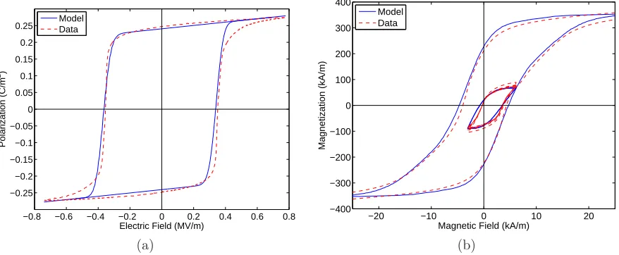
In this paper, we focus on the development of highly efficient implementation and inversion techniques for the homogenized energy model for subsequent use in high speed design and control algorithms. We employ this technique due to its physical basis, which permits correlation of parameters with measured properties of data [24], and it capability to characterize a wide range of physical behaviors including closure of bi-ased minor loops in quasistatic regimes, thermal relaxation or creep, reversible behavior prior to switching, and temperature-dependent dynamics. Details regarding the framework including a discussion of how it compares and contrasts to Preisach models, can be found in [24]. Throughout, the algorithms will be com-pared using parameters obtained from data fits to PLZT (a ferroelectric) and Terfenol-D (a ferromagnetic). Representative fits are shown in Figure 1.
This work extends previous work in a number of regards. We establish here that the continuity of field-polarization or field-magnetization relations is maintained with approximation but also demonstrate numerical integration or quadrature stepsize requirements to achieve this continuity numerically. This di-rectly impacts subsequent inversion algorithms. We then discuss new quadrature techniques to improve the continuity of approximate relations for improved inversion and control implementation. As an extension to [2], we develop look-up table and rational Chebyshev techniques to improve the implementation for cer-tain applications and we develop implementation techniques to characterize the displacements generated by ferroelectric or ferromagnetic rods. Finally, we design highly efficient algorithms to construct inverse models that incorporate thermal relaxation for subsequent linear control design.
In Section 2 we introduce implementation algorithms for nonlinear and hysteretic field-polarization/field-magnetization relations and in Section 3 we employ these relations to construct algorithms for displacements generated by ferroelectric or ferromagnetic rods. The implementation of the inverse model is addressed and numerically demonstrated in Section 4.
−0.8 −0.6 −0.4 −0.2 0 0.2 0.4 0.6 0.8
−0.25 −0.2 −0.15 −0.1 −0.05 0 0.05 0.1 0.15 0.2 0.25
Electric Field (MV/m)
Polarization (C/m
2)
Model Data
−20 −10 0 10 20 −400
−300 −200 −100 0 100 200 300 400
Magnetic Field (kA/m)
Magnetization (kA/m)
Model Data
(a) (b)
2
Homogenized Energy Model
2.1
Theoretical Development
We summarize here the homogenized energy model for ferroelectric and ferromagnetic materials [1, 24–26, 29, 30]. To simplify the discussion we develop it in the context of ferroelectric materials and note that analogous relations hold for ferromagnetic compounds. We note that this is a multiscale approach in which mesoscopic behavior is quantified via energy principles and a macroscopic model is subsequently constructed via stochastic homogenization techniques. The macroscopic ferroelectric model is
P(E;x+) =
Z ∞
0
Z ∞
−∞
νc(Ec)νI(EI)[P(E+EI;Ec;x+)]dEIdEc (1)
where P denotes the polarization, E is the electric field, Ec denotes the coercive field value at which the
dipoles change orientation,EI quantifies the interaction field due to dipole interactions, andP is a mesoscale
polarization relation. The two model parameters Ec and EI are assumed to vary throughout the material
according to the densitiesνc and νI. The densities are constrained by the the physical relations:
1. bothνc andνI are bounded by decaying exponentials,
2. νc is strictly positive,
3. νI is symmetric about 0, and
4. R∞
0 νc(Ec)dEc= 1,
R∞
−∞νI(EI)dEI = 1.
(2)
The integrals in (1) are solved numerically via quadrature relations, that is,
P(E;x+) =
Nc X
i=1
NI X
j=1
νc(Ec[i])νI(EI[j])wc[i]wI[j]P(E+EI[j];Ec[i];x+[i, j]) (3)
wherewc andwI give the quadrature weights.
The kernelP is modeled via energy principles. The mesoscopic Helmholtz energy is taken to be
ψ(P) =
η(P+PR)2/2, P ≤ −PI
η
2(PI−PR)
P2
PI −
PR
, |P|< PI
η(P−PR)2/2, P ≥PI
(4)
wherePI =PR−Ec/ηdenotes the positive inflection point at which the dipoles switch orientation,PRis the
local remanence polarization, andη is the reciprocal slope ∂E
∂P. This energy relation is plotted in Figure 2.
The Gibbs free energy
G=ψ−EP (5)
balances this internal Helmholtz energy with the electrostatic energy; i.e., work performed by the applied external field. As detailed in [24], where the Legendre transform properties of the Gibbs energy are discussed, Gis a function of the independent variableE and the dependent variableP.
For regimes in which thermal relaxation is negligible, direct minimization of (5) yields the kernel
P(E+EI, x+) =
E+EI
η + 2PRx+−PR (6)
where x+ = 1 for positively oriented dipoles and x+ = 0 for negatively oriented dipoles. For algorithm
development, x+ is set to 1 whenever E+EI > Ec and is set to 0 wheneverE+EI < −Ec. Thermal
activation is manifested by dipoles having sufficient thermal energy to switch states before a minima of the Gibbs energy is eliminated. To quantify this, the Gibbs energy is balanced with the relative thermal energy through Boltmann’s relation. It is shown in [24, 25, 30] that the resulting kernel is
P ψ + P P− P I R P
Figure 2: Helmholtz energy function (4)
wherex+∈[0,1] denotes the fraction of positively oriented dipoles and
hP+i=
R∞ PI Pexp
−G(E+EI,P)V
kT
dP R∞
PI exp
−G(E+EI,P)V
kT
dP , hP
−i=
R−PI
−∞ Pexp
−G(E+EI,P)V
kT
dP R−PI
−∞ exp
−G(E+EI,P)V
kT
dP (8)
are the average polarizations associated with positive and negative dipole orientations. HereV is the meso-scopic volume being modeled, kis Boltmann’s constant, and T is the temperature in degrees Kelvin. The evolution of dipole fractions is governed by the differential equation
˙
x+ =−p+−x++p−+(1−x+) (9)
where the likelihoodsp+− andp−+of a dipole switching from positive to negative, or vice-versa, are
p+−=
exp
−G(E+EI,PI)V
kT
dP
τ(T)R∞
PI exp
−G(E+EI,P)V
kT dP p −+= exp
−G(E+EI,−PI)V
kT
dP
τ(T)R−PI
−∞ exp
−G(E+EI,P)V
kT
dP (10)
and τ quantifies the material and temperature-dependent relaxation time. It is noted in [24] that whereas these likelihood relations are commonly employed in practice, they must be treated as approximate in a statistical sense.
2.2
Implementation Formulation
The average polarization relations (8) and switching likelihood relations (10) are computationally expensive to compute, especially since they must be computed at each quadrature point and each time step. However, the choice of a piecewise quadratic Helmholtz energy, as opposed to a single fourth-order polynomial or other function, poses several advantages. One advantage is it allows these average polarizations and switching likelihoods to be expressed in a more computationally efficient form. To simplify notation, letEe=E+EI
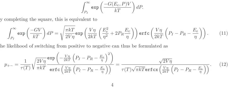
denote the effective field. Consider the integral Z ∞
PI exp
−G(Ee, P)V
kT
dP.
By completing the square, this is equivalent to Z ∞ PI exp −GV kT dP = s πkT 2V ηexp
V η 2kT E2 e
η2 + 2PR
Ee η erfc V η 2kT
PI−PR−
Ee
η
. (11)
The likelihood of switching from positive to negative can thus be formulated as
p+−=
1 τ(T) r 2V η πkT exp
−2V ηkT
PI−PR−Eηe
2
V η P
−P −Ee
=
√
2V η
τ(T)√πkT V η P −P −Ee
Similarly, the fundamental theorem of calculus may be applied to R∞ PI Pexp
−GV kT
dP to obtain
hP+i=
√
2kT
√
πV ηerfcx
V η
2kT
PI −PR−Eηe
+Ee
η +PR. (13)
Similar approaches may be taken for the other average polarization and switching likelihood. Introducing the change of variables
zp=
s V
2kT η(−E−EI−Ec), zn = s
V
2kT η(E+EI−Ec) (14)
yields the relations
p+−=
1 τ(T) r 2V η πkT 1 erfcx(zp)
, hP+i=
s 2kT πV η
1 erfcx(zp)
+E+EI
η +PR.
p−+ =
1 τ(T) r 2V η πkT 1 erfcx(zn)
, hP−i=−
s 2kT πV η
1 erfcx(zn)
+E+EI
η −PR.
(15)
Since the scaled complementary error functions appear in both switching likelihoods and average polar-izations, the value need only be computed once instead of twice. To this end, define
pos= 1
erfcx(zp)
, neg= 1
erfcx(zn)
. (16)
The model can then be expressed as
P(E;x+) = E
η −PR+
Nc X i=1 NI X j=1
wc[i]wI[j] (x+(pos+neg+k1)−neg) (17)
where
wc[i] =
p
2kT /πV ηνc(Ec[i])wc[i], wI[j] =νI(EI[j])wI[j], k1=PR
p
2πV η/kT .
We note that the relations Z ∞
−∞
Z ∞
0
νc(Ec)νI(EI)dEcdEI = 1,
Z ∞
−∞
Z ∞
0
νc(Ec)νI(EI)EIdEcdEI= 0
were used to simplify the equations. These result directly from the physical constraints (2). Similarly the evolution of dipole fractions is given by
˙
x+=
1
k2
(−x+(pos+neg) +neg) (18)
where
k2=τ(T)
s πkT 2V η.
The differential equation (18) may be solved by any number of numerical differential equations routines. For example, using the backward Euler method,x+ is computed at each time step as
x+(t+ ∆t) =
k2
∆tx+(t) +neg k2
∆t+neg+pos
. (19)
A more accurate, but also slightly more computationally intensive approximation, can be solved by assuming
a digital system. In this case, the differential equation is a linear constant coefficient equation, and can be solved analytically to obtain
x+(t+ ∆t) = neg
neg+pos+
x+(t)− neg
neg+pos
exp
−∆tk
2
(neg+pos)
. (20)
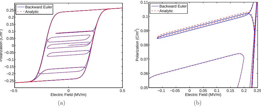
Whereas more accurate, the difference between the solution values provided by this formulation and (19) is typically not significant. For example, Figure 3 shows the results of both methods for an example input and parameter set (in this case, taken to match the ferroelectric material PLZT). As can be seen in the magnified version, the difference between the methods is minimal. For most applications, (19) is considered sufficiently accurate and we employ this approach due to its greater computational simplicity.
The formulations given here can significantly improve the run-time of the algorithm as compared with a more direct implementation of the equations in Section 2.1. However, in many cases better performance is still required. This leaves two options: reduce the number of quadrature points or consider additional approximation strategies.
2.3
Quadrature and the Continuity of P
It is observed that the computation time of the model is directly proportional toNcNI, the number of
quadra-ture points. One may hope to improve computational performance by reducing the number of quadraquadra-ture points. However, this exaggerates actual or apparent discontinuities in the outputP.
By definition of the integral, the model (1) is continuous and differentiable. However, the model with quadrature (3) does not retain this smoothness. Since (3) is composed of finite sums,P is smooth if and only ifP is smooth for every quadrature point. Clearly for the negligible relaxation case (6),P is discontinuous, and its value changes by 2PR at the coercive pointE+EI =Ec. Thus,P containsNcNI finite jumps, each
of size 2PRνc(Ec[i])νI(EI[j])wc[i]wI[j] fori= 1. . . Nc, j= 1. . . NI.
For the relaxation case, it can be shown that P(E;x+) is a continuous function. However, a plot of
P(E;x+) (or ratherM(H;x+) since the parameters come from a least-squares data fit to a Terfenol-D rod)
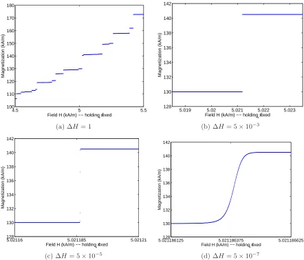
shows that extremely small stepsizes may be required to resolve this continuity. Figure 4(a) shows a plot of M(H;x+) for various values ofH where the statex+ was held fixed; i.e., each plotted sample was obtained
by inputting the givenH to the model with the same value ofx+. The step between each input value of
H was 1 A/m, and the function appears to be discontinuous. However, zooming in on one of these regions shows that the function is in fact continuous (see Figures 4(b) – 4(d)). Note, however, that it took a ∆H
−0.5 0 0.5
−0.25 −0.2 −0.15 −0.1 −0.05 0 0.05 0.1 0.15 0.2 0.25
Electric Field (MV/m)
Polarization (C/m
2)
Backward Euler Analytic
−0.1 −0.05 0 0.05 0.1 0.15 0.2 0.25
0.05 0.06 0.07 0.08 0.09 0.1 0.11
Electric Field (MV/m)
Polarization (C/m
2)
Backward Euler Analytic
(a) (b)
4.5 5 5.5 100
110 120 130 140 150 160 170 180
Field H (kA/m) −− holding x
+ fixed
Magnetization (kA/m)
5.019 5.02 5.021 5.022 5.023 128
130 132 134 136 138 140 142
Field H (kA/m) −− holding x
+ fixed
Magnetization (kA/m)
(a) ∆H= 1 (b) ∆H= 5×10⁻³
5.02116 5.021185 5.02121
128 130 132 134 136 138 140 142
Field H (kA/m) −− holding x
+ fixed
Magnetization (kA/m)
5.021186125128 5.021186375 5.021186625
130 132 134 136 138 140 142
Field H (kA/m) −− holding x+ fixed
Magnetization (kA/m)
(c) ∆H= 5×10⁻⁵
(d) ∆H= 5×10⁻⁷
Figure 4: Plot ofM(H;x+) for 6 intervals of composite 4-point Gaussian quadrature on each density. For
each value ofH,x+ was held fixed; thus the plots represent a single timestep of the model for various input
levels. The parameters in these plots were taken from a least-squares fit to Terfenol-D data.
approximately 10 orders of magnitude below H to resolve the function in detail. It is unrealistic to expect such steep slopes to be resolved numerically. In practice, therefore, we must allow for the relaxation model to be discontinuous as well.
Model-based control applications require a smooth model response. As detailed in [24], the relaxation model limits to the negligible relaxation model as V
kT → ∞. Since, the jump discontinuities in the negligible
relaxation model are of height 2PRνc(Ec[i])νI(EI[j])wc[i]wI[j] for i= 1. . . Nc, j = 1. . . NI, we expect that
for large V
kT the “discontinuities” of the relaxation model will also be approximately this height. Thus, the
actual or apparent discontinuities may be minimized by minimizingνc(Ec[i])νI(EI[j])wc[i]wI[j].
One way to increase smoothness is thus to increase the number of quadrature points. If the densities remain unchanged and the number of quadrature points is doubled, thenwc[i]wI[j] is halved for alli, j. This
cuts the size of the jump in half. However, computation time is proportional to the number of quadrature points, so halving the height of the jumps in this way doubles the computation time. This is clearly undesirable. A better situation can be obtained if care is taken on how the quadrature is performed.
Since both νc andνI are bounded by decaying exponentials, quadrature may be performed on a finite
a quadrature rule is applied to each subinterval. Typically, all the subintervals are taken to be equally spaced and this approach was used in the plots given previously. However, equally spaced subintervals are merely a convenience – there is no theoretical reason why one subinterval cannot be bigger than an-other. In particular, if the region is partitioned such that the integral over each subinterval is equal, then νc(Ec[i])νI(EI[j])wc[i]wI[j] will be on the same order of magnitude for alli, j. (Equality is not obtained
becauseνc andνI vary on the interval and because for a general quadrature formula not all the weights are
equal.) This has the effect of leveling out the jumps, decreasing the big ones while the small ones increase. The result is depicted in Figure 5.
The required number of quadrature points is often determined by accuracy and smoothness requirements. This approach can reduce the number of quadrature points needed for a given smoothness, resulting in significant computational savings.
2.4
Approximation Methods for Improved Computational Performance
Reduction of quadrature points alone is not always sufficient to achieve the desired performance of the relaxation model. Significant savings can also be obtained by introducing numerical approximations into the kernel itself. Exploration of the kernel shows that the majority of computation time is spent in the calculation of (16), and we thus focus on methods to approximateposandneg. This is equivalent to approximating
f(z) = 1
erfcx(z) (21)
since bothposand negrequire this function for different values of z. The rest of the model is employed in the manner detailed previously.
2.4.1 Look-up Tables
The simplest approach conceptually is to storef(z) in a table for values of interest and approximateposand neg by looking up the table value nearestzp andzn, respectively. At the cost of memory, this reduces the
complexerfcxcalculation to a simple index calculation and memory access. The indexes into the lookup
4.5 5 5.5
100 110 120 130 140 150 160 170 180
Field H (kA/m) −− holding x
+ fixed
Magnetization (kA/m)
Equally spaced intervals Unequally space intervals
Figure 5: Comparison ofM(H;x+) for 6 intervals of composite 4-point Gaussian quadrature on each
table may also be calculated efficiently. Lethbe the difference inzbetween two elements of the table, and letℓbe thezvalue corresponding to the first (lowest) table entry. Then define
˜ Ec[i] =
Ec[i]
h s
V 2kT η−
ℓ
h, i= 1. . . Nc, E˜I[j] =
EI[j]
h s
V
2kT η, j= 1. . . NI, E˜ = E
h V 2kT η.
Most of these calculations can be performed offline. Only ˜E needs to be computed at each time step and this may be done outside the loops over the quadrature points. Once these values are obtained, the table index is obtained by rounding
pos index=−E˜−E˜I[j]−E˜c[i], neg index= ˜E+ ˜EI[j]−E˜c[i] (22)
to the nearest integer. These values must be checked against the table bounds. An index less than zero signifies a zero should be given instead of a value from the table, whereas an index greater than or equal to the table size implies that the linear approximation should be used instead. Note that the linear approximation for largerzcan be adjusted to take the table index (preferably without rounding) instead of thezp orzn as
input as well, allowing ˜Ec and ˜EI to replace the memory taken by the original quadrature points.
The lookup table approach has several advantages: it is conceptually straightforward, algorithm run-time is independent of table size (within architecture-dependent limits), and approximation error goes to zero as the table size increases. Even relatively small tables yield decent accuracy as illustrated in Table 3 for an example input field. Here it is seen that even 100 table elements produce a root-mean-square error less than approximately 0.25% of the remanence polarization, and at 10,000 table elements this error was reduced to approximately 0.002% of the remanence polarization. Note that 10,000 elements is less than 100 KB of memory when using IEEE double precision floating point numbers. Finally, table values do not need to be recalculated if material properties (i.e., temperature) change. However, there are architectures where this moderate amount of memory is unattainable, or where memory access is too slow. For these cases, we alternatively consider polynomial approximations.
2.4.2 Rational Chebyshev Approximation
If the look-up table approximation is infeasible, the function f(z) can instead by approximated by a poly-nomial or a rational function
Rmk(z) =
pm(z)
qk(z)
(23)
wherepis a polynomial of degreemandqis a polynomial of degree k. HereRmk is chosen such that
maxw(z)f(z)−Rmk(z)
(24)
is minimized. This is referred to as a rational Chebyshev or minimax approximation, and is the approach used to implementerfcinternally as well. While it can be shown that a unique minimix approximation exists for allmandk, computation of these approximations in numerically intensive [22]. However,f(z) does not depend on the material parameters or inputs. Thus, the minimax approximation can be calculated in advance and made available to the code for any choice of parameters. Methods to calculate these approximations using the Remez (also called Remes) algorithm are available in bothMathematicaandMaple, alleviating the user from coding minimax algorithms themself.
Like the look-up table, the minimax approximation is applied on a bounded interval. Additionally, the weight functionw(z) must be specified. The obvious choices arew(z) = 1 for absolute error orw(z) = 1/f(z) for relative error. For larger z, relative error is a better metric for controlling error. However, for smallz calculation of relative error is problematic sincef(z)−→0. Thus, we let
w(z) = min
1, erfc(z) exp(−z2)
(25)
We consider two methods to improve the accuracy of the approximation. One approach is to increasem and/ork while the other is to use multiple polynomials over smaller regions instead of a single polynomial over the whole region. Higher degree polynomials increase computational effort in floating point operations whereas adding more polynomials increases conditional statements and control logic. An optimal balance of these is architecture-dependent. As an example, letf(z) be approximated as
f(z)≈
0 z <−3
Rℓ(z) =
pℓ0+pℓ1z+pℓ2z2+pℓ3z3
qℓ0+qℓ1z+qℓ2z2 −3≤z≤ −
1 2
Rh(z) =
ph0+ph1z+ph2z2+ph3z3
qh0+qh1z+qh2z2 −
1
2 < z≤25
mz+b z≥25.
(26)
This employs two minimax approximations with a degree 3 numerator and degree 2 denominator where the regions for each approximation were chosen so that the minimax error (24) is approximately the same. This holds the error (24) below 4×10⁻⁴
for allz <25. Since this accuracy is well above the limits imposed by IEEE double precision floating point numbers, further computational savings may be realized by transforming Rℓ(z) andRh(z) into continued fraction form, namely
Rℓ(z) =aℓ0const+aℓ0linz+
bℓ1
z+aℓ1+z+bℓa2ℓ2
, Rh(z) =ah0const+ah0linz+
bh1
z+ah1+z+bha2h2
. (27)
Note that for each of these evaluations only 1 multiply, 2 divides, and 5 additions are required. The values of the relevant coefficients are given in Table 1.
2.4.3 Method Comparisons
Neither method is optimal for all situations. However, the look-up table approach is generally the most efficient in terms of run-times and accuracy. Tables 2 and 3 list the run times and errors for an example input. Parameter values were taken to match the ferroelectric material PLZT, and the temperature was assumed to remain constant. It can be seen that either the look-up table or polynomial approximations should almost always be preferred over the exact formulations. As expected, the look-up table approach outperforms the polynomial approach. The run time for various table sizes is not shown because as long as the table was kept small enough to fit in the processor’s cache, the run-time was not significantly affected by the size of the table. In cases where the modest memory requirement cannot be achieved, the rational Chebyshev approximation should be used. This takes slightly longer and/or provides less accuracy than the look-up table approximation, but reduces the memory requirement to a handful of values. It is doubtful the memory will ever pose an issue on a conventional processor. Regions where it may prove unattainable are on embedded microprocessors and custom designed field programmable gate arrays (FPGAs) or application specific integrated circuits (ASICs). Rational Chebyshev approximations are a natural choice for these applications.
3
Displacement Model
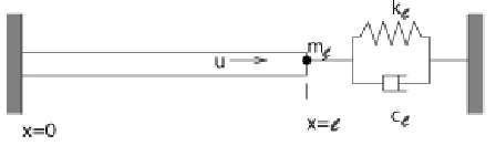
Whereas polarization or inductance/magnetization can sometimes be measured, it is often necessary to formulate the model in terms of displacement instead of polarization. Any such extension requires knowledge of the geometry of the transducer. Rods or beams can be treated with a one-dimensional transducer model, whereas more general shapes require higher-dimension models. As detailed in [24], both nanopositioning stages employed in common atomic force microscope designs and magnetic transducers employed for high speed milling utilize ferroelectric and ferromagnetic rods that are clamped at one end and subject to damped restoring forces at the other. Hence we illustrate the model for a rod of lengthℓ and cross sectional areaA as depicted in Figure 6. The end massmℓ with dampingcℓ and stiffnesskℓ encompass adjacent transducer
m 1.771048244745112288944163714 b 0.0705327380461303718160865974 aℓ0const 1.05305341778847673369961876455 aℓ0lin 0.141908467579507101523861449079
aℓ1 0.652521450575033268529746994429 bℓ1 2.05040334028682659509776710501
aℓ2 -0.139674180341575164555785667908 bℓ2 2.88659338549683880846513610339
ah0const 0.0568934411527620915320982226406 ah0lin 1.77070610668997459554647064088
ah1 -12.9327277303294522316468471279 bh1 0.269387658595592656676548244377
ah2 16.4152526433497348583844713265 bh2 216.983649137026313567944222991
Table 1: Coefficients for the minimax approximation given in (26).
Intel Xeon Intel Xeon (64 bit) Intel Pentium-M
1.7 GHz 3.8 GHz 2.16 GHz
256 KB L2 Cache 2 MB L2 Cache 2 MB L2 Cache
Negligible relaxation 10,748 62,725 31,969
algorithm
Relaxation – full numerical 429 1801 1276
precision
Relaxation – look-up table 5344 14,923 14,226
approximation
Relaxation – polynomial 4997 11,674 12,177
approximation (26)
Table 2: Time steps per second computed by each algorithm for three different computer architectures (averaged from 1 million time step). Polynomial approximation was performed using the continued fraction form (27) of the example polynomial given in (26). Look-up tables were computed for−6≤z≤25. In all cases, the model was run with 40 quadrature points for each distribution (1600 total).
Peak error (% of remanence) RMS error (% of remanence)
Look-up table (100 table elements) 0.65860% 0.25593%
Look-up table (1000 table elements) 0.063883% 0.0055925%
Look-up table (10,000 table elements) 0.0020362% 0.00019354%
Polynomial approximation (26) 0.5377% 0.1647%
Table 3: Approximation error for an example input using parameters obtained for PLZT. Polynomial ap-proximation was performed using the continued fraction form (27) of the example polynomial given in (26); look-up tables were computed for −6 ≤z ≤25, anderfcx was implemented directly as exponential and error function evaluations, with the linear approximation utilized for largez. Forty quadrature points were given for each distribution (1600 total)
Figure 6: Rod used to construct overall model. The end mass mℓ, stiffness kℓ and damping cℓ represent
It is shown in [24] that the constitutive relation for the induced stress is given by
σ=Y ε+Cε˙−a1(P−P0)−a2(P−P0)2 (28)
whereY is the Young’s modulus of the transducer,Cis the Kelvin-Voight damping coefficient,P0is the point
the material is poled around,a1 anda2 are constants of proportionality relating the induced polarization to
mechanical force, andP =P(E;x+) is given in (3).
Due to the distributed nature of the device, partial differential equation models have been developed in [24, 27] to characterize the device dynamics. However, for a number of motivating applications, it has been shown that because forces and fields are uniform in space, strains and hence displacements are also uniform thus permitting the use of ordinary differential equation representations. In this case, the strain is given by
ε(t) =u(t)
ℓ (29)
whereu(t) denotes the displacement of the rod tip at timet. A force balance yields
md
2u
ℓ
dt2 +c
duℓ
dt +kuℓ=α1(P−P0) +α2(P−P0)
2 (30)
whereρis the density of the rod and
m=ρAℓ+mℓ, c=
CA
ℓ +cℓ, k=
Y A
ℓ +kℓ,
α1=Aa1, α2=Aa2.
Further details as well as models for additional geometries may be found in [24, 27].
The solution to this differential equation can be obtained with a variety of numerical methods. However, variable-step methods require thatP be known at arbitrary times, which in turn requires that the homoge-nized energy model be solved at arbitrary times. This is typically not feasible in practice. We thus focus on fixed time-step methods. Of these, the most accurate approximation for a given stepsize may be obtained by assuming thatP is fixed between time steps so (30) can be solved analytically. This is an approximation, since thermal effects dictateP will vary with time even ifEis constant; however, all other fixed step methods implicitly make similar assumptions and include additional approximation error as well.
The approximation of (30) depends on the relation of c2
m2 to
4k
m. First, to simplify notation let
v=a1
m(P−P0) +
a2
m(P−P0)
2
. (31)
Herevis assumed to be a constant, although the value of the constant changes at each time step. Additionally, let
˜
k= k
m, ˜c=
c
m.
If ˜c2>4˜kthen the solution is given by
u(t) =b1exp
−12
˜
c+
q ˜
c2−4˜k
t
+b2exp
−12
˜
c−
q ˜
c2−4˜k
t
. (32)
Again, to simplify notation letz=pc˜2−4˜k. Lettingu(0) =u
0 and ˙u(0) =u1gives
b1=
1 2
1− ˜c
z u0−
v ˜ k
−1
zu1, b2=
1 2
1 + c˜
z u0−
v ˜ k
+1
zu1. (33)
Substitution into (32) and collection of like terms yields
u(t) =1
2
1−˜c
z
exp
−1
2(˜c+z)t
+
1 + ˜c z
exp
−1
2(˜c−z)t u0− v ˜ k +1 exp
−1(˜c−z)t
−exp
−1(˜c+z)t
u1+
v .
If we assume the step ∆t is fixed, then we can define the six constants
d1=1
2
1−cz˜
exp
−12(˜c+z) ∆t
+
1 + ˜c
z
exp
−12(˜c−z) ∆t
, d3= 1
k(1−d1),
d2= 1
z
exp
−12(˜c−z) ∆t
−exp
−12(˜c+z) ∆t
,
d4=
1 4
˜
c2
z −z exp
−1
2(˜c+z) ∆t
−exp
−1
2(˜c−z) ∆t
, d6=−
d4
˜
k.
d5=
1 2
1 + c˜
z
exp
−12(˜c+z) ∆t
+
1−z˜c
exp
−12(˜c−z) ∆t
,
(35)
In terms of these constants, the solution of the rod model for ˜c2>4˜kis approximated by
u(t+ ∆t) =d1u(t) +d2u(t) +˙ d3v(t+ ∆t),
˙
u(t+ ∆t) =d4u(t) +d5u(t) +˙ d6v(t+ ∆t).
(36)
A similar approach can be taken for the other two cases. If ˜c2 = 4˜k, we again obtain (36) except with
the constants given by
d1=
1 + c˜
2∆t
exp
−c2˜∆t
, d4=−k∆texp
−2˜c∆t
,
d2= ∆texp
−˜c2∆t
, d5=
1−2˜c∆t
exp
−˜c2∆t
,
d3=
1
k(1−d1), d6=−
d4
˜
k .
(37)
Finally, if ˜c2<4˜k, the values for the constants are
d1=exp
−2˜ct cosz 2∆t
+c˜
zsin
z 2∆t
, d4=−1
2
z+˜c
2
z
exp
−2˜ct
sinz 2∆t
,
d2= 2
zexp
−˜c2t
sinz 2∆t
, d5=exp
−2˜ct cosz 2∆t
−cz˜sinz 2∆t
,
d3=
1
k(1−d1), d6=−
d4
˜
k.
(38)
Thus, the rod model costs only six multiplies and four additions per iteration, plus three multiplications and two additions for the calculation ofv. That is, the rod model computation is essentially free when compared to the computational cost of the homogenized energy model.
4
Inverse Model
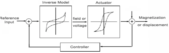
As discussed in Section 1, one method to accurately control a smart material actuator involves the use of an inverse model or compensator in the manner depicted in Figure 7. Linearization in this manner allows simple control techniques including PI/PID and LQR designs to be utilized over the entire range of the actuator. Given a specified displacement, we wish to determine the field necessary to bring the actuator to that value. Such inverse compensators have previously been explored for the negligible relaxation model in [8, 24]. Here we consider a method that works for both the relaxation and negligible relaxation models.
The rod model may be inverted analytically. Solving (36) forv yields
v(t) = 1
d3
u(t)−dd1
3
u(t−∆t)−dd2
3
˙
Figure 7: Control configuration utilizing an inverse model and a linear control law.
Oncevhas been determined, the required polarization can be determined from the quadratic formula, namely
b
P(t) =P0−
α1
2α2 ±
sα
1
2α2
2
+mv(t)
a2
(40)
as long asα26= 0. Ifα2 is 0, the equation is linear and the solution is
b
P(t) =P0+ m
α1
v(t). (41)
Note that forα26= 0, either polarization value is acceptable, as both give equivalent displacements. However,
to minimize the effects of modeling error, a single branch should always be utilized.
A definition of the inverse homogenized energy model is the following: given any valid statex+ and any
specifiedPb within the operating range of the material, determineEsuch thatP =P. Unlike the rod model,b however, it is not feasible to invert (3) analytically. Thus, we reformulate the problem as numerical root finding, namely determining the valueE such that for a givenx+ andPb,
P(E;x+)−Pb= 0. (42)
We note that this function is monotone inE (holdingx+ fixed). However, as discussed in Section 2.3, the
function may contain a finite number of simple jumps.
4.1
Discontinuous Root Finding
If (42) was continuously differentiable, the secant method would provide nearly optimal convergence to the solution in terms of function evaluations [10]. However, for a discontinuous function it may not converge. The bisection method will converge, but often this convergence is slow. Methods exist which combine bisection with interpolation to attempt to improve this rate; see [3] for example. However, we observe better performance by exploiting the monotone nature of the function to directly improve the convergence of the bisection method.
The bisection method, or any other method which utilizes it, requires both that the root be bounded and that the function change signs within the bounds. For a monotone function, these requirements are the same. Theoretical bounds onE may be computed by considering the case when all dipoles have switched. In these cases (all dipoles positive or all negative),E can be determined analytically. The required value of E is by necessity between these extreme cases, namely
η(Pb−PR)≤E≤η(Pb+PR). (43)
However, direct application of the bisection method with these bounds yields slow convergence because the bounds are large.
not smooth, this may not converge. However, the monotone nature of the function dictates that the secant method will always step in the correct direction. Thus, on each iteration either the secant method does not step far enough, in which case a better approximation to E is obtained, or it steps too far. In this latter case, the iterations have crossed over the root value and provide a bound on the root. We therefore apply the secant method to (42) first. If there is sufficient relaxation or the valuePb does not lie near any discontinuities, we obtain rapid convergence. If the secant method fails to converge, the secant iterations themselves are utilized to determine the bound on the root which can then be given to bisection to find the actual root. These bounds are typically much tighter than (43), which improves the convergence of the bisection method. For the purposes of our algorithm, failure to converge in the secant method is defined as
|P(Ei;x+)−Pb| ≥ |P(Ei−2;x+)−Pb|, for alli≥3 (44)
where Ei is the value of E determined by the ith iteration of the secant method. Such a definition is a
heuristic to detect failure quickly without penalizing a single poor step.
The secant method requires an initial approximation to the derivative to compute its first iteration. One such approximation is 1/ηwhich is the derivative if no dipoles are switching. The actual derivative may be much larger than this, but will never be smaller. Another approximation involves using the previous two time steps of the model in a manner analogous to how the secant method itself approximates derivatives. This approximation is simply ∆P/∆E, where ∆P is the difference in P(E;x+) for the previous two time
steps and ∆E is the corresponding differences inE. The latter approximation is deemed more accurate and is utilized when the previous two time steps are known. When this is not the case, 1/ηis utilized as the initial derivative. The computed derivative value should also be checked against this lower limit on each iteration of the secant method, to trap some errors that may arise with the subtraction of nearly equal numbers.
4.2
Validation and Performance
The performance of the inverse model is largely dependent on the material parameters being utilized. More relaxation, smaller variances inνc andνI, and slowly changing reference inputs generally yield better
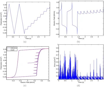
per-formance than small relaxation, largely varying distributions, or rapidly varying inputs. As an example, consider the inverse model for the stepped polarization shown in Figure 8(a). The parameters are specified as those estimated for PLZT to obtain the model fit in Figure 1(a). Ten intervals with 4-point Gaussian quadrature are utilized for each distribution and the time step is ∆t= 0.001. As can be seen, the inverse model accounts for the relaxation in the device, decreasing the electric field as appropriate to hold the po-larization constant. The error between the specified and actual values is small – five orders of magnitude below the remanence polarization.
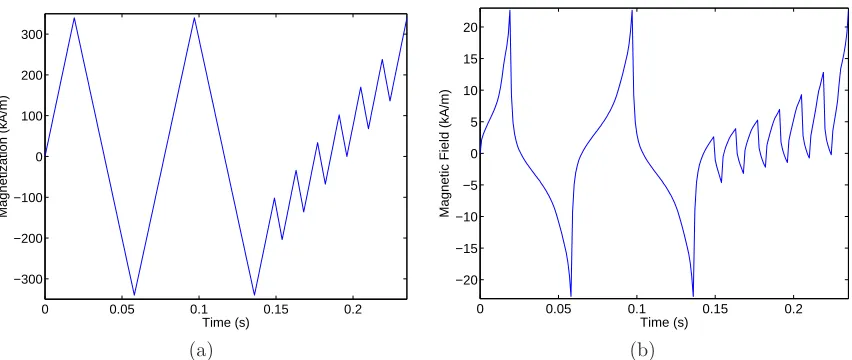
The results in Figure 8 were computed with a small tolerance for the secant and bisection methods. Accuracy and effort for various tolerance levels are compiled in Table 4. Note that the algorithm makes efficient use of computation; reasonable accuracy levels may be obtained with only 2 function evaluations (evaluations of the forward homogenized energy model) per iteration on average, or 5 in the worst case. However, this efficiency is dependent on the input. Figure 9(a) shows an input polarization which changes at roughly an order of magnitude higher rate. Using the same material parameters and time step on this input yields the results in Figure 9(b) and Table 5. The same accuracy level as before requires almost 5 function evaluations on average and 16 in the worst case. While increased, this is still easily attainable. The level of effort also depends on the material being modeled. Scaling Figure 9(a) to an appropriate level and applying parameters for a Terfenol-D rod yields the results in Figure 10 and Table 6. The Terfenol-D parameters require greater work for the same level of accuracy, but relatively speaking they are able to achieve a greater accuracy than that achieved in the PLZT case.
Finally, we note that these observations apply directly to the case when displacement is utilized as input. Figure 11 and Table 7 show the accuracy and level of effort for the Terfenol-D parameters with strain (displacement) as an input. The tolerance for the root finding algorithm was also specified in terms of displacement in this case, withP(E;x+) input to the rod model on each iteration of secant or bisection to
0 0.5 1 1.5 2 2.5 3 −0.25
−0.2 −0.15 −0.1 −0.05 0 0.05 0.1 0.15 0.2 0.25
Time (s)
Polarization (C/m
2)
0 0.5 1 1.5 2 2.5 3 −0.6
−0.4 −0.2 0 0.2 0.4 0.6
Time (s)
Electric Field (MV/m)
(a) (b)
−0.4 −0.2 0 0.2 0.4 0.6
−0.25 −0.2 −0.15 −0.1 −0.05 0 0.05 0.1 0.15 0.2 0.25
Electric Field (MV/m)
Polarization (C/m
2)
reference result
0 0.5 1 1.5 2 2.5 3 0
0.1 0.2 0.3 0.4 0.5 0.6 0.7 0.8 0.9 1
Time (s)
Error (
µ
C/m
2)
(c) (d)
Figure 8: (a) Reference polarization and (b) electric field E given by the inverse model with parame-ters estimated for PLZT. (c) Comparison of the resulting polarizationP and the reference polarizationPb. (d) Absolute error|Pb−P|.
Tolerance Function Evaluations (Average) Function Evaluations (Maximum)
PR×10−2= 0.0024 1.0855 3
PR×10−3= 0.00024 1.2667 4
PR×10−4= 2.4×10⁻⁵ 2.0157 5
PR×10−5= 2.4×10⁻⁶ 3.5423 9
PR×10−6= 2.4×10⁻⁷ 4.8066† user-defined
0 0.05 0.1 0.15 0.2 −0.25
−0.2 −0.15 −0.1 −0.05 0 0.05 0.1 0.15 0.2 0.25
Time (s)
Polarization (C/m
2)
0 0.05 0.1 0.15 0.2 −0.5
−0.4 −0.3 −0.2 −0.1 0 0.1 0.2 0.3 0.4 0.5
Time (s)
Electric Field (MV/m)
(a) (b)
Figure 9: (a) Reference polarization and (b) electric field E given by the inverse model with parameters estimated for PLZT.
Tolerance Function Evaluations (Average) Function Evaluations (Maximum)
PR×10−2= 0.0024 2.8776 10
PR×10−3= 0.00024 3.9286 13
PR×10−4= 2.4×10⁻⁵ 4.8027 16
PR×10−5= 2.4×10⁻⁶ 7.9252† user-defined
PR×10−6= 2.4×10⁻⁷ 9.3187† user-defined
Table 5: Effort to compute the inverse model in terms of average and maximum number of function evalua-tions for various error tolerances, using parameters for PLZT and the input given in Figure 9(a). †denotes that due to discontinuities, some time steps did not converge within the specified tolerance, and only those that did are averaged. In these cases, the maximum number of function evaluations was the user-specified maximum.
0 0.05 0.1 0.15 0.2
−300 −200 −100 0 100 200 300
Time (s)
Magnetization (kA/m)
0 0.05 0.1 0.15 0.2
−20 −15 −10 −5 0 5 10 15 20
Time (s)
Magnetic Field (kA/m)
(a) (b)
Tolerance Function Evaluations (Average) Function Evaluations (Maximum)
MR×10−2= 3400 2.8673 9
MR×10−3= 340 5.4354 16
MR×10−4= 34.0 10.7143 22
MR×10−5= 3.40 14.2993 25
MR×10−6= 0.340 17.2279 29
Table 6: Effort to compute the inverse model in terms of average and maximum number of function evalua-tions for various error tolerances, using parameters for Terfenol-D and the input given in Figure 10(a).
5
Concluding Remarks
In this paper, we have provided a computationally efficient formulation of the homogenized energy model suitable for use in nonlinear model-based control designs, parameter estimation routines, and inverse-compensator based-control for ferroelectric and ferromagnetic actuators. We have also demonstrated that the inverse model accurately and efficiently compensates for ferroelectric and ferromagnetic hysteresis in an open-loop of feedforward manner without requiring anya priori knowledge of the reference input. The
re-0 0.02 0.04 0.06 0.08 0.1
−20 −10 0 10 20 30 40 50
Time (s)
Displacement (microns)
(a)
0 0.02 0.04 0.06 0.08 0.1
−2 −1 0 1 2 3 4 5
Time (s)
Magnetic Field (kA/m)
0 0.02 0.04 0.06 0.08 0.1
0 2 4 6 8 10 12 14 16 18
Time (s)
Displacement Error (pm)
(b) (c)
Figure 11: Results for the combined inverse model with parameters estimated for a Terfenol-D rod. (a) Spec-ified displacementuband (b) magnetic fieldH provided by the inverse algorithms. (c) Absolute error|bu−u|
Error Average Maximum tolerance model evaluations model evaluations
1 micron 2.1240 8
100 nm 2.2880 9
10 nm 6.5170 19
1 nm 11.6500 22
100 pm 14.7040 25
10 pm 17.6930 29
Table 7: Effort to compute the inverse model in terms of average and maximum number of function evalua-tions utilizing parameters estimated for a Terfenol-D rod and the reference displacement given in Figure 11(a).
sulting inverse algorithms are capable of achieving reasonable accuracy at speeds of 500 - 3000 timesteps per second on a conventional processor, depending on the number of quadrature points and material parameters. With a resolution of 10 timesteps per cycle, this would allow periodic inputs at the rate of 50 - 300 Hz. Multiprocessor and/or custom integrated circuit (FPGA/ASIC) implementations should allow this rate to be greatly increased and are currently under investigation.
ACKNOWLEDGMENTS
This research was supported by a United States Department of Education GAANN fellowship and the Air Force Office of Scientific Research under the grant AFOSR-FA9550-04-1-0203.
References
[1] T.R. Braun, R.C. Smith, and M.J. Dapino, “Experimental validation of a homogenized energy model for magnetic after-effects,”Applied Physics Letters, 88(12), 2006.
[2] T.R. Braun and R.C. Smith, “Efficient Implementation Algorithms for Homogenized Energy Models,” Continuum Mechanics and Thermodynamics, 18(3-4), pp. 137-155, 2006.
[3] R.P. Brent, Algorithms for Minimization without Derivatives, Prentice-Hall, Englewood Cliffs, N.J., 1973.
[4] W.J. Cody, “Rational chebyshev approximations for the error function,”Mathematics of Computation, 23(107), pp. 631-637, 1969.
[5] M.J. Dapino, R.C. Smith, L.E. Faidley, and A.B. Flatau, “A coupled structure-magnetic model for magnetostrictive transducers,”Journal of Intelligent Material Systems and Structures, 11(2), pp. 134-152, 2000.
[6] P. Ge and M. Jouaneh, “Modeling hysteresis in piezoceramic actuators,” Precision Engineering, 17, pp. 211-221, 1995.
[7] P. Ge and M. Jouaneh, “Tracking control of a piezoceramic actuator,”IEEE Transactions on Control Systems Technology, 4(3), pp. 206-209, 1996.
[8] A.G. Hatch, R.C. Smith, T. De, and M.V. Salapaka, “Construction and experimental implementation of a model-based inverse filter to attenuate hysteresis in ferroelectric transducers,”IEEE Transactions on Control Systems Technology, 14(6), pp. 1058-1069, 2006.
[10] C.T. Kelley,Iterative Methods for Linear and Nonlinear Equations,SIAM, Philadelphia, 1995.
[11] J.A. Main and E. Garcia, “Design impact of piezoelectric actuator nonlinearities,”Journal of Guidance, Control and Dynamics, 20(2), pp. 327-332, 1997.
[12] J.A. Main and E. Garcia, “Piezoelectric stack actuators and control system design: strategies and pitfalls,”Journal of Guidance, Control, and Dynamics, 20(3), pp. 479-485, 1997.
[13] J.A. Main, E. Garcia and D.V. Newton, “Precison position control of piezoelectric actuatorss using charge feedback,”Journal of Guidance, Control, and Dynamics, 18(5), pp. 1068-73, 1995.
[14] J.A. Main, D. Newton, L. Massengil and E. Garcia, “Efficient power amplifiers for piezoelectric appli-cations,”Smart Structures and Materials, 5(6), pp. 766-775, 1996.
[15] J.E. Massad and R.C. Smith, “A domain wall model for hysteresis in ferroelastic materials,”Journal of Intelligent Material Systems and Structures, 14(7), pp. 455-471, 2003.
[16] I.D. Mayergoyz,Mathematical Models of Hysteresis, Springer-Verlag, New York, 1991.
[17] S. Mittal and C-H. Meng, “Hysteresis compensation in electromagnetic actuators through Preisach model inversion,”IEEE/ASME Transactions on Mechatronics, 5(4), pp. 394-409, 2000.
[18] J.M. Nealis and R.C. Smith, “H∞control design for a magnetostrictive transducer,” Proceedings of the
42nd IEEE Conference on Decision and Control, pp. 1801-1806, 2003.
[19] J.M. Nealis and R.C. Smith, “Model-based robust control design for a magnetostrictive transducer operating in hysterestic and nonlinear regimes,” IEEE Transactions on Control Systems Technology, 15(1), pp. 22-39, 2007.
[20] W.S. Oates, P. Evans, R.C. Smith, and M.J. Dapino, “Experimental implementation of a nonlinear control method for magnetostrictive transducers,” Proceedings of the 46th IEEE conference on Decision and Control, to appear.
[21] W.H. Press, S.A. Teukolsky, W.T. Vetterline, B.P. Flanner, Numerical Recipes in C, 2nd Edition, Cambridge University Press, New York, 1992.
[22] A. Ralston, “Rational Chebyshev approximation”,Mathematical Methods for Digital Computers, Vol. 2, John Wiley and Sons, New York, pp. 268-284, 1967.
[23] G. Robert, D. Damjanovic and N. Setter, “Preisach modeling of piezoelectric nonlinearity in ferroelectric ceramics,”Journal of Applied Physics, 89(9), pp. 5067-5074, 2001.
[24] R.C. Smith,Smart Material Systems: Model Development, SIAM, Philadelphia, 2005.
[25] R.C. Smith, M.J. Dapino, T.R. Braun and A.P. Mortensen, “A Homogenized energy framework for ferromagnetic hysteresis,”IEEE Transactions on Magnetics, 42(7), pp. 1474-1769, 2006.
[26] R.C. Smith, M.J. Dapino and S. Seelecke, “A free energy model for hysteresis in magnetostrictive transducers,”Journal of Applied Physics, 93(1), pp.458-466, 2003.
[27] R.C. Smith, A.G. Hatch, T. De, M.V. Salapaka, R.C.H. del Rosario, and J.K. Raye,“Model Develop-ment for Atomic Force Microscope Stage Mechanisms,”SIAM Journal on Applied Mathematics, 66(6), pp. 1998-2026, 2006.
[28] R.C. Smith and J.E. Massad, “A unified methodology for modeling hysteresis in ferroic materials,” Pro-ceedings of the 2001 ASME Design Engineering Technical Conferences and Computer and Information in Engineering Conference, Vol 6, Pt B, pp. 1389-1398, 2001.
[30] R.C. Smith, S. Seelecke, Z. Ounaies and J. Smith, “A free energy model for hysteresis in ferroelectric materials,”Journal of Intelligent Material Systems and Structures, 14(11), pp. 719-739, 2003.
[31] G. Song, J. Zhao, X. Zhou and J.A. Abreu-Garci, “Tracking control of a piezoceramic actuator with hysteresis compensation using inverse Preisach model,”, IEEE/ASME Transactions on Mechatronics, 10(2), pp. 198-209, 2005.
[32] X. Tan and J.S. Baras, ”Modeling and control of hysteresis in magnetostrictive actuators,”Automatica, 40(9), pp. 1469-1480, 2004.
[33] X. Tan, R. Venkataraman and P.S. Krishnaprasad, “Control of hysteresis: Theory and experimental results,” Smart Structures and Materials 2001, Proceedings of the SPIE, Volume 4326, pp. 101-112, 2001.