Fine-Scale Estimation of Location of Birth from Genome-Wide Single-Nucleotide Polymorphism Data

(1)

INVESTIGATION

Fine-Scale Estimation of Location of Birth

from Genome-Wide Single-Nucleotide

Polymorphism Data

Clive J. Hoggart,*,1,3_{Paul F. O}_’_Reilly,*,1_{Marika Kaakinen,}†_{Weihua Zhang,* John C. Chambers,*},‡,§ Jaspal S. Kooner,†,_{** Lachlan J. M. Coin,*},2_{and Marjo-Riitta Jarvelin*},†,††,‡‡ *Department of Epidemiology and Biostatistics, Imperial College, London W2 1PG, United Kingdom,†Institute of Health Sciences and Biocenter Oulu, University of Oulu, FIN-90014 Oulu, Finland,‡Ealing Hospital National Health Service (NHS) Trust, Middlesex UB1 3HW, United Kingdom,§Imperial College Healthcare NHS Trust, London W12 1NY, United Kingdom, **National Heart and Lung Institute, Imperial College London, Hammersmith Hospital, London W12 0HS, United Kingdom,††National Institute for Health and Welfare, FI-00271 Helsinki, Finland, and‡‡Medical Research Council–HPA Centre for Environment and Health, Imperial College, Faculty of Medicine, London W2 1PG, United Kingdom

ABSTRACTSystematic nonrandom mating in populations results in genetic stratification and is predominantly caused by geographic separation, providing the opportunity to infer individuals’birthplace from genetic data. Such inference has been demonstrated for individuals’country of birth, but here we use data from the Northern Finland Birth Cohort 1966 (NFBC1966) to investigate the characteristics of genetic structure within a population and subsequently develop a method for inferring location to a finer scale. Principal component analysis (PCA) shows that while the first PCs are particularly informative for location, there is also location information in the higher-order PCs, but it cannot be captured by a linear model. We introduce a new method, pcLOCATE, which is able to exploit this information to improve the accuracy of location inference. pcLOCATE uses individuals’PC values to estimate the probability of birth in each town and then averages over all towns to give an estimated longitude and latitude of birth using a fully Bayesian model. We apply pcLOCATE to the NFBC1966 data to estimate parental birthplace, testing with successively more PCs and finding the model with the top 23 PCs most accurate, with a median distance of 23 km between the estimated and the true location. pcLOCATE predicts the most recent residence of NFBC1966 individuals to a median distance of 47 km. We also apply pcLOCATE to Indian individuals from the London Life Sciences Prospective Population Study (LOLIPOP) data, andfind that birthplace is predicated to a median distance of 54 km from the true location. A method with such accuracy is potentially valuable in population genetics and forensics.

P

RINCIPAL component analysis (PCA) has been used ex-tensively to control for population structure (Priceet al.

2006) and describe genetic diversity. It has been applied to worldwide allele frequency data of human populations (Cavalli-Sforza et al. 1993) and more recently to dense SNP data to illustrate population structure in Europe (Lao

et al.2008; Novembreet al.2008), India (Reichet al.2009), and China (Xuet al.2009). Recent analyses of populations sampled across Europe demonstrated that genetic data could be used to predict place of birth to within a few hun-dred kilometers (Novembreet al.2008).

Here we introduce a new Bayesian method, pcLOCATE, for predicting location of origin. We apply the method to the Northern Finland Birth Cohort 1966 (NFBC1966), which includes genome-wide data and location information on 2823 unrelated individuals born in 1966 in the two north-ernmost provinces of Finland, Oulu, and Lapland (Sabatti

et al. 2008), and to The London Life Sciences Prospective Population Study (LOLIPOP), comprising genome-wide data and location data on 1574 individuals living in West London (UK) and born in India (Chamberset al.2010). We compare

Manuscript received October 10, 2011; accepted for publication November 8, 2011 Supporting information is available online at http://www.genetics.org/content/ suppl/2011/11/18/genetics.111.135657.DC1.

1_{These authors contributed equally to this work.}

2_{Present address: Department of Genomics of Common Disease, School of Public}

Health, Imperial College London, Hammersmith Hospital, London, United Kingdom.

3_{Corresponding author: Department of Epidemiology and Biostatics, Imperial College,}

(2)

the accuracy of pcLOCATE with the approach of Novembre

et al. (2008), in which linear models for longitude and latitude were employed with linear and quadratic effects for the first two PCs (Novembre et al. 2008). PCA of the NFBC1966 data shows that higher-order PCs appear to con-tain information on location, but not through a simple lin-ear relationship. pcLOCATE was developed to utilize as many PCs as are informative without assuming a linear re-lationship between PCs and location. We test the accuracy of the two methods with inclusion of successively more PCs. While the linear method gains little in accuracy with the addition of PCs of order greater than two, pcLOCATE can exploit the information in higher-order PCs and is thus able to achievefiner-scale estimates. By applying pcLOCATE to two population samples with very different charac-teristics we are able to gain insight into the general appli-cability of pcLOCATE to human populations. Fine-scale estimation of individuals’ location may lead to improved methodology in population genetics and could have imme-diate application in forensics through assisting in perpetra-tor identification.

Applying PCA to NFBC1966 also allows us to study the population structure in Northern Finland, one of the most keenly studied population isolates. The settlement of Fin-land has been characterized by early and late settlement regions (Peltonen et al.1999). The early settlement region comprises the coastal regions of the south and west, which have likely been inhabited for many millennia. The late set-tlement began in the 16th century with migration into the interior of the country from a small area in the southeast of Finland (Peltonenet al.1999). The late settlement was char-acterized by the establishment of isolated rural populations by relatively small numbers of founding individuals. Strong founder effects are also evident in India; within Indian an-cestral groups there is evidence of excess allele sharing and allele frequency differences between groups are larger than in Europe (Reichet al.2009). Before applying pcLOCATE to the NFBC1966 and LOLIPOP data sets we investigate how the results from PCA applied to the NFBC1966 data compare to what is known about the demographic history of North-ern Finland.

Materials and Methods

Genotype data

NFBC1966 aimed to recruit all individuals born in Northern Finland in 1966 and contains genotype data from the Illuminia 300K chip for 329,091 SNPs in 4793 individuals. A subset of 61,917 SNPs was selected on which we performed PCA; the SNPs were selected such that call rate .99.5%, minor allele frequency.1%, and Hardy–Weinburg equilibrium P-value .0.005 and thinned to satisfy an LD criteria in which r2 _,_{0.2 for all pairs of SNPs to prevent}

overrepresentation of regions of high LD. The PCs generated were used in all analyses. For 2823 individuals we have

records of their parents’town of birth and their most recent town of residence, where town refers to any clustered hu-man settlement. Informed consent from all study subjects was obtained using protocols approved by the Ethical Com-mittee of the Northern Ostrobothnia Hospital District. See Sabattiet al.(2008) for further details.

The LOLIPOP study is a population-based cohort study of Indian, Asian, and European white males and females, aged 35–75 years, recruited from West London. Country of birth was recorded with other biomedical information, and blood was taken for genetic analysis. The Illumina Human610 was used to genotype the LOLIPOP individuals. Genotype and location data were available for 1574 individuals from the study that were born in India. Samplewise quality control (QC) included removing duplicates, gender information error, low sample call rate (,95%), related individuals, and ethnic outliers. SNP-wise QC included removing SNPs with low call rate (,95%), low frequency (minor allele frequency,0.01), and low Hardy–Weinberg equilibrium P-values (,1026_).

SNPs were thinned prior to PCA according to their correlation with nearby SNPs, using the pruning option in PLINK (Purcell

et al.2007). PCA was calculated with the smartpca program in the EIGENSOFT package (v3.0) (Pattersonet al.2006). All participants provided written consent for the genetic studies. The LOLIPOP study is approved by the Ealing and St Mary’s Hospitals Research Ethics Committees. See Chambers et al.

(2010) for further details.

pcLOCATE model

pcLOCATE assumes individuals are from discrete areas, which we refer to as towns, and uses an individual’s PCs to estimate the probability of them originating from each of the towns in a country or region. Location is predicted as latitude and longitude by calculating a weighted average of the latitude and longitude of each town, weighted according to the town-of-birth probabilities. Thus the model does not impose a linear relationship between PCs and location but does exploit the local smoothness in PC variation. pcLOCATE uses the top p

PCs to estimate origin (either birthplace or most recent resi-dence); the model assumes that thekth PC (k= 1, . . . ,p) value of an individual originating from towntj(j= 1, . . . ,m)

is normally distributed with mean mjk and precision (= 1/

variance) ljk. We use the model to predict parental

birth-place, birthbirth-place, and most recent residence. When modeling parental birthplace, we generalize the likelihood such that each individual’s PC values contribute two independent observations to the likelihood, one at their father’s town of birth and one at their mother’s town of birth. In the remain-der of this section we describe the model for predicting pa-rental birthplace in detail; the models for birthplace and most recent residence follow straightforwardly from this descrip-tion, replacing location of the mother’s and father’s birthplace with the location of the individual’s birthplace or most recent residence.

Conditional on parental birthplace and utilizing theﬁrstp

(3)

pðxiPjmj;lj;Ti1¼tj1;Ti2¼tj2Þ ¼ Qp

k¼1

Nðxikjmj1k;lj1kÞNðxikjmj2k;lj2kÞ;

where xiP = (xi1, . . . ,xip) are the ﬁrstpPC values of

in-dividuali,Ti1andTi2are the towns of birth of the parents of

i, and N is the normal distribution parameterized by the town- and PC-speciﬁc means and precisions given by ele-ments of the matrices mandl.

The location of birth of the parents of a new individual is estimated by Bayesian model averaging in which the latitude and longitude of each town is weighted by the posterior probability of being born in each town. When making a prediction of parents’birthplace, we estimate a sin-gle location (assuming one parent) rather than considering all possible pairs of locations for the two parents. Therefore, the expectation of the location of birth of the parents of a new individual z with PC values z = (z1, . . . , zp) is

estimated by

Eðlocation of birth of parents of zÞ

¼ Pm

j¼1

L_jpTz ¼ tjjz;D;a;b

¼k Pm

j ¼ 1

Ljp

Tz ¼ tjjD Qp

k¼1

pzkjTz ¼ tj;D;ak;bk

;

(1)

whereDis the data (the PCs and towns of birth of parents of allNindividuals in the sample),Tzis the town of birth of the

parent ofz,Ljis the latitude and longitude of towntj,kis the

normalizing constant, andaandbare vectors of hyperpara-meters described in Equation 2 below.

The likelihood of observingz’s PCs in each town, required for the product in (1), is obtained by integrating out the unknown town-speciﬁc means and precisions. For robust-ness and to obtain an analytic solution for the likelihoods in (1), we assignmjkandljktheir conjugate prior,

pðmjk;ljkÞ ¼Nðmjkjm0;n0ljkÞGa

l_jkja_k;b_k; (2)

where Ga is the gamma distribution parameterized by shape parameteraand scale parameterb(mean and variance of distribution: a/b and a/b2_{, respectively). The likelihood}

terms in the product in equation (1) can then be calculated as

pzkjTz¼tj;D;ak;bk

¼RNðzkjmjk;ljkÞ

pðm_jk;ljkÞ Q

i2SjNðxikjmjk;ljkÞ pðxSjÞ

dm_jkdljk

¼RNðzkjmjk;ljkÞpðmjk;ljkjxSj;ak;bkÞdmjkdljk;

(3)

whereSjindicates individuals with a parent born in towntj

and xsj are the PC values of these individuals [where both parents of an individual are born in tj, their PC value

con-tributes two observations to the product in (3)]. Takingn0=

0 (see below for discussion on choice of prior parameters) and integrating yields

¼St zkjxjk;

nj

akþnj=2

njþ1

b_kþ ð1=2Þnjs2_jk

;2akþnj !

(4)

(Bernardo and Smith 1994), where St is Student’s distribu-tion with probability density funcdistribu-tion given by

Stðxju;t;gÞ}

h

1þg21tðx2uÞ2

i₂_ðgþ1Þ=2

and nj is the number of parents born in town tj,

xjk¼ ð1=njÞ P

a2Sjxakandnjs

2 jk¼

P

a2Sjðxak 2 xjkÞ

2

.

The probability of town of origin prior to observing PCs is assumed to reﬂect the relative population sizes of the towns and is thus given by a conjugate multinomial Dirichlet model; with an uninformative Dirichlet prior in which all parameters = 1

2 and the observations are the number of

births in each town, this probability is given by

pTz¼tjjD

¼1=2þnj

m=2þN: (5)

Therefore, the location of birth of parents of zis estimated by substituting (4) and (5) into (1). By averaging over towns we exploit the smooth variation of the PCs with ge-ography. The most recent residence of individuals in the cohort (recorded at age 31) is estimated by replacing paren-tal birthplace with individual residence in (1) and (2).

The parameters of the prior distribution (2) were de-termined as follows. The gamma prior onljkhas meanak/bk,

and this was set to the mean precision of PCkacross all towns. The degree of shrinkage toward the mean is controlled byak;

the larger ak is, the greater the shrinkage, with each unit

increase in ak having the relative effect of two observations

from the prior. We setak= 50 to balance the requirements of

robust estimation and local adaptivity. We compare our results with those achieved by usingak= 0 (no shrinkage) andak=

1000 (hard shrinkage and thus minimal local adaptivity). Sen-sitivity analyses showed that prediction was better without shrinkingmjkto the mean PC values, so we assigned the

pa-rameter aﬂat vague prior by settingn0= 0.

We compare pcLOCATE with the model used in Novem-bre et al. (2008); to implement the method, we ﬁnd the rotation of PCs 1 and 2 that maximizes the correlation be-tween the rotated vectors and latitude and longitude. The rotated elements are given by

v1 v2 ¼

cosu 2sinu sinu cosu

z1

z2

;

whereuis chosen to maximize

fðuÞ ¼corðn1;longitudeÞ þcorðn2;latitudeÞ:

(4)

birthplace with linear, quadratic, and interaction effects for the rotated PCs 1 and 2 values,

latitude_¼fð1Þ 0 þf

ð1Þ

1 n1þfð21Þn21þfð 1Þ

5 n1n2þeð1Þ

longitude_¼fð2Þ 0 þfð

2Þ

5 n1n2þeð2Þ;

where thefs are the regression coefﬁcients and the es are normally distributed random errors. To compare with pcLO-CATE when using more than theﬁrst two PCs, we extend the model above to also include linear and quadratic effects for PCs 3 and above. We also compare with a model with the same formulation as above but that includes only linear effects for the PCs.

In evaluating all models, overﬁtting is avoided by out-of-sample prediction whereby each individual’s town-of-birth probabilities are calculated with that individual removed from the estimation. Thus, for example, in the evaluation of pcLOCATE, for individual ithe estimation of town- and PC-speciﬁcm’s andl’s is conditional on the PCs and towns of birth of parents of all individuals except i. The distance between two points measured by latitude and longitude was calculated using the Haversine formula (Gellert et al.

1989).

Results

Population structure in Northern Finland

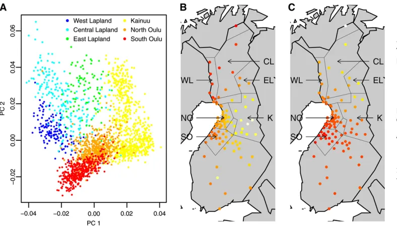
We began by inspecting theﬁrst two PCs in relation to early and late settlement regions, since those are the most likely to highlight any signiﬁcant distinction according to settle-ment region. The NFBC1966 region has been divided into six linguistic/geographic regions: three early settlement regions, North Oulu, South Oulu, and West Lapland; and three late settlement regions, Kainuu and East and Central Lapland (Jakkula et al. 2008; Sabatti et al. 2008); the regions are marked in Figure 1, B and C. Figure 1A displays a scatter plot of PC 1 against PC 2 values for all individuals whose parents were born in the same region (2136 individ-uals), colored according to the region of parental birth. The plot shows that individuals from the same region are nearby on the PC1/PC2 plane and that the clockwise order of the regions corresponds to their order geographically. However, the relationship between distance on the PC1/PC2 plane and geographic distance is nonlinear. We also note that the regions do not correspond to distinct clusters; genetic distance, as measured by PCs 1 and 2, appears to be driven by separation-by-distance rather than separation-by-region. The rotation of PCs 1 and 2 found to maximize correlation with latitude and longitude was–26.

Next we calculated the average intensities of PCs 1 and 2, separately, at each town over all individuals with a parent born in the town; thus, each individual’s PC was counted twice, once at their mother’s place of birth and once at their father’s. Parental birthplace was recorded as the town clos-est to their location of birth. Figure 1, B and C, illustrates the

results for PC 1 and 2, respectively. Each point represents the average intensity of the PC for that town; the redder the color is, the lower the average PC intensity. Figure 1B shows that PC 1 exhibits a smooth linear southeast/northwest gra-dient, taking highest values in Kainuu in the southeast of the NFBC1966 region and decreasing with distance from Kai-nuu. PC 2 also exhibits a smooth linear gradient (Figure 1C) but from southwest to northeast. Both PCs exhibit greater north–south variation in the eastern, late settlement, regions than in the western, early settlement, regions, in-dicating greater genetic diversity in the late settlement regions, in line with previous studies (Peltonen et al.

1999; Jakkula et al. 2008). The late settlement region of Kainuu in the southeast is at one end of the PC 1 spectrum, while individuals in East and Central Lapland, also late set-tlement, are as distant from Kainuu in terms of PC 1 as those from the early settlement regions of North and South Oulu. Furthermore, towns in the early settlement regions of North and South Oulu are close to one another on the first two PCs, while towns in West Lapland, also considered an early settlement region, are relatively distant from Oulu on both PCs. Thesefindings support the notion that the genetic strat-ification reflects geographic separation rather than separa-tion by region or early/late settlement.

Intensity plots of PCs 3–20 (Supporting Information, Fig-ure S1andFigure S2) show that these PCs also indicate no early/late settlement distinction but, unlike the ﬁrst two PCs, do not exhibit a linear relationship with geography. They can, for instance, take values at opposite ends of the PC range at nearby towns. For example, Salla and Kuusamo have mean values of PC 6 in the 5th and 95th percentiles of PC 6 (t-test for difference of PC 6 means,P,2·10216_),

respectively, despite being,100 km apart. In fact, Kuusamo is a known internal isolate of Finland, whose present pop-ulation is thought to trace back to 40 founding families from the 17th century (Varilo et al.2003). Such differenti-ation in the values of higher-order PCs at nearby towns suggests that higher-order PCs may be informative for

ﬁne-scale geographic location and that implementing a non-linear model for PCs may best capture the location informa-tion in them.

Application of pcLOCATE to NFBC1966

We first predict parental birthplace and individuals’ most recent residence by pcLOCATE without the PCs in the model, thus estimating the town of birth probabilities from the prior alone (Equations 1 and 5), which should reflect the popu-lation sizes of each town only. Then, starting with PC 1, we added successively higher-order PCs until the addition of further PCs reduces the predictive accuracy of the model. By adding thefirst 25 PCs wefind that the pcLOCATE model is optimized for these data with the inclusion of thefirst 23 PCs.

(5)

predicted and true birthplace for both parents, and Figure 2B shows that between the predicted and true most recent residence of each individual. The mean and median accu-racy of pcLOCATE increases as more PCs are included, to a maximum at 23 PCs for parental birthplace prediction and 8 PCs for most recent residence, while the linear model (Novembre et al. 2008) shows negligible improvement in accuracy with more than theﬁrst 2 PCs. The mean distance between true and predicted parental birthplace is 47 km for pcLOCATE and 57 km for the linear model, while the me-dian distance is 23 km for pcLOCATE and 45 km for the linear model. The mean distance between true and pre-dicted most recent residence is 67 km for pcLOCATE and 71 km for the linear model, while the median distance is 47 km for pcLOCATE and 59 km for the linear model. Figure 2, C and D, compares the cumulative distribution of the dis-tance between the true and estimated location of the

best-ﬁtting models for each method. It shows that pcLOCATE gives substantially better ﬁne-scale prediction than the linear model. For example, pcLOCATE predicts parental birthplace to within 10 km for 37% of individuals’parents and to within 50 km for 68% of individuals’parents, while the linear model predicts 3% to within 10 km and 52% to within 50 km. For most recent residence pcLOCATE predicts 20% of individuals to within 10 km and 50% to within 50 km, while the corre-sponding proportions for the linear model are 3% and 40%, respectively. When both methods have large errors, the linear model performs slightly better, which can be explained by its predictions being more tightly located around the center of the NFBC66 region, thus limiting the size of the errors. Over-all, pcLOCATE gave a more accurate prediction of parental birthplace than the linear model for 80% of parents and a more accurate prediction of most recent residence for 70% of individuals. At-test for difference in mean distance between predicted and actual location of parental birthplace and most recent residence, comparing pcLOCATE and the linear model,

gaveP,2·10216_{for both comparisons. Application of the}

method of Novembre et al. (2008) with only linear effects for the PCs gave marginally inferior prediction in compar-ison with the accuracy achieved by the full model, reduc-ing the mean and median accuracy of the best-ﬁtting model by,1 km.

The six regions of NFBC1966 have markedly different population distributions. Figure 3 summarizes the predictive accuracy of pcLOCATE in the six regions. Figure 3A shows a box plot of the distance between the predicted and true location of parental birthplace stratiﬁed by region of birth of the parents (for individuals with both parents born in the same region), while Figure 3B shows the same box plots but for prediction of most recent residence. Despite the differ-ences in population distributions, the accuracy of pcLOCATE is similar in all six regions, which suggests that results from pcLOCATE are robust to heterogeneity in population density. The greater accuracy of the models estimating parental birthplace may be a consequence of increased migration levels since the Second World War. The error distribution of pcLOCATE predictions of parental birthplace and most recent residence are shown inFigure S3, A and B.

Application of pcLOCATE to LOLIPOP

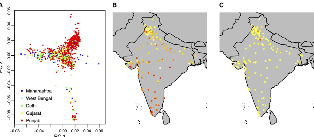
Figure 4 summarizes the variation in PCs 1 and 2 in the LOLIPOP cohort. Figure 4A shows a plot of PC 1 vs. PC 2 values for individuals from theﬁve most populous regions in the study population, accounting for 90% of the sample, and Figure 4, B and C, shows the mean intensities of PC 1 and PC 2 in each region. It is notable from these plots that the re-lationship between genetic variation and geography is less linear than that observed in NFBC1966.

Figure 5A shows a plot of the number of PCs in the pcLOCATE and linear models against the mean and median distance between the predicted and true birthplace for both parents. Again, the accuracy of pcLOCATE increases as more

(6)

PCs are included, whereas the accuracy of the linear model improves little with the addition of more PCs. Figure 5B compares the cumulative distribution of the distance be-tween the true and the estimated location of the best-ﬁtting models for each method. Again pcLOCATE gives substan-tially betterﬁne-scale prediction than the linear model. For example, pcLOCATE predicts birthplace to within 50 km for 47% of individuals, while the linear model predicts only 12% to within 50 km. A t-test for difference in mean dis-tance between predicted and actual birthplace, comparing pcLOCATE and the linear model, gave P,2·10216_{. The}

error distributions of pcLOCATE predictions of birthplace are shown in Figure S4. Application of the method of Novembre et al. (2008) with only linear effects for the PCs resulted in inferior prediction in comparison with the accuracy achieved by the full model, reducing the mean accuracy by5 km.

If pcLOCATE was used in conjunction with the LOLIPOP data to infer birthplace of individuals from the general Indian population, then the prior used in this analysis would need to be replaced with one that was representative of the population density of India. However, in our application the prior distribution reﬂects the geographic distribution of the study population and so is appropriate for estimating the

location of individuals within this study. It would also be preferable to ascertain a sample of individuals that was representative of the geographic distribution of Indians as it has been shown that PCA can be biased by uneven geo-graphical sampling (Novembre and Stephens 2008; McVean 2009). NFBC1966 is not subject to such bias as it aimed to recruit all individuals born in Northern Finland in 1966 and therefore the sample should reﬂect the population distribution.

Effect of shrinkage of town-speciﬁc precision

Shrinkage of town-speciﬁc precision is controlled bya. The effects of varying a on the accuracy of pcLOCATE in the analyses of the NFBC1966 and LOLIPOP data are shown in Figure S5and Figure S6. These plots show that for the LOLIPOP data shrinking the town-speciﬁc precisions, ljk’s,

using eithera= 50 ora= 1000 provides superior accuracy to that achieved by usinga= 0. However,a= 50 anda= 0 are optimal for the NFBC1966 data, while hard shrinkage, a= 1000, has a detrimental effect on prediction. Therefore, the choice ofa= 50 achieves both the objectives of robust estimation, which is of importance in the LOLIPOP data, and local adaptivity, which is of importance in the NFBC1966 data.

Figure 2 Predictive accuracy of pcLOCATE and linear model ap-plied to NFBC1966. (A) Mean (solid lines) and median (dashed lines) predictive accuracy for pa-rental birthplace of pcLOCATE (red) and the linear model (blue) by number of PCs. (B) Mean (solid lines) and median (dashed lines) predictive accuracy for most re-cent residence of pcLOCATE (red) and the linear model (blue) by number of PCs. (C) Cumula-tive distribution of the distance between true and estimated pa-rental birthplace of the best-ﬁtting models of pcLOCATE (red) and the linear model (blue). (D) Cumu-lative distribution of the distance between true and estimated most recent residence of the best-ﬁtting models of pcLOCATE (red) and the linear model (blue).

(7)

Discussion

Our results suggest that the early and late settlement regions, and six linguistic/geographic regions, used here and elsewhere (Jakkulaet al.2008; Sabattiet al. 2008) do not correspond to genetic subpopulations. However, we assessed population structure using PCA, where SNPs were selected to be uncorrelated, and we therefore did not exploit information on haplotype variation. Nevertheless, a recent study that investigated variation in LD between individuals from different regions of Finland found that while individ-uals from the NFBC1966 region exhibited higher LD on average than those from the rest of Finland, there were no discernible distinctions within the NFBC1966 region (Jakkulaet al.2008).

The smooth variation in the top two PCs could be explained by the late settlement deriving from migrants from across the early settlement regions, migrating accord-ing to geographic location. However, it had been believed that the late settlement derives from a small group of people

in the southeast of the country (Peltonenet al.1999; Norio 2003), which would suggest that the smooth variation in the top two PCs is due to migration since the late settlement period. We cannot infer the direction of migration from PCs (McVean 2009; François et al.2010) and so cannot distin-guish between these two hypotheses in the present study. We found that some higher-order PCs take extreme values in some towns, although we cannot make inference on popu-lation history from these observations as it has been shown that the patterns of variation in higher-order PCs can be markedly different from the patterns of migration that oc-curred (Novembre and Stephens 2008). For example, under simulation, even when migration is constant and homoge-neous in time and space, higher-order PCs tend to exhibit wave-like patterns of variation with location.

Our model for predicting location of origin, pcLOCATE, is better able to capture the relationship of many PCs with geog-raphy than a simple linear model for latitude and longitude with linear and quadratic PC effects (Novembreet al.2008), providing improved predictive accuracy. pcLOCATE is similar

Figure 4 Variation in PCs 1 and 2 in the LOLIPOP cohort. (A) PC 1vs.PC 2 values, colored according to region of birth for individuals from theﬁve most populous regions in the study population, accounting for 90% of the sample. (B and C) Mean intensities of PC 1 (B) and PC 2 (C) in each region, from a scale of white (high) to red (low).

(8)

to the linear discriminant analysis method (Egeland et al.

2004) recently employed to differentiate between several rural villages in three European countries (O’Dushlaine

et al.2010). Like pcLOCATE, the method uses PCs for pre-diction and assumes that PC values are normally distributed in each town. However, while O’Dushlaine et al. (2010) estimate birthplace as the most probable village using the

ﬁrst three PCs, our estimate is a location in terms of longi-tude and latilongi-tude derived from a weighted average of the posterior probabilities over all towns, which exploits the smooth variation in PC intensity with geography and all of the data. Furthermore, once PCs have been computed, pcLOCATE is fully Bayesian and utilizes as many PCs as are informative. By successively adding higher-order PCs we improve the accuracy of our location estimates, until maximized, demonstrating that many PCs can be informa-tive for location.

In applying pcLOCATE to the NFBC1966 and LOLIPOP data sets we found that the method can predict individual origin to a ﬁne scale. In the NFBC1966 analysis, 68% of individuals had parental birthplace predicted to within 50 km of the true location, while 50% of the sample had most recent residence predicted to within 50 km. The birthplaces of 47% of individuals from the LOLIPOP data were predicted to within 50 km. The results from applying pcLOCATE to population samples with different population densities and sample selection criteria suggest that the method may be widely applicable to human populations. The NFBC1966 study attempted to recruit all births in the region in 1966, whereas the LOLIPOP individuals used in our study are individuals born in India currently residing in West London (UK).Fst, a measure of population differentiation, between

North and South Oulu and West Lapland within the early settlement region of NFBC1966 is between 0.001 and 0.003 and between Central and East Lapland and Kainuu within the late settlement region is between 0.002 and 0.004 (Jakkula et al. 2008). These values are comparable to the genetic differentiation across Europe, where average Fst=

0.004 between geographic regions within Europe (Novem-breet al.2008). However,Fstbetween early and late

settle-ment regions is as high as 0.006 (Jakkulaet al.2008). The average Fstbetween subpopulations within India has been

estimated to be 0.011 (Reich et al. 2009), thus substan-tially higher than within Finland and Europe.

Founder effects, genetic isolation, and limited migration in Northern Finland (Peltonen et al. 1999; Jakkula et al.

2008) are reﬂected in the accuracy by which both pcLOCATE and the method of Novembreet al.(2008) estimate parental birthplace and most recent residence in NFBC1966. The method of Novembre et al. (2008) gave a mean distance between true and predicted parental birthplace of 57 km; this compares with an accuracy of a few hundred kilometers when applied to individuals distributed across Europe (Novembre et al.2008) and a mean accuracy of280 km when applied to the LOLIPOP data. The disparity between the accuracy of the methods when applied to the NFBC1966

and LOLIPOP data is also dependent on geographic scales over which the two data sets are derived, and therefore the larger the potential errors.

As well as for future applications in population genetics we suggest that our ﬁndings could prove valuable for the

ﬁeld of forensics now, particularly in Finland and India. DNA left at a crime scene could be used to estimate the perpetrator’s most likely region of origin, providing a lead for an investigation with little other information and no match to a criminal DNA database. In addition, we believe that our method is likely to be applicable to many similar populations around the world, especially those with recent founding effects and/or low migration over many genera-tions. The accuracy achieved in this study may be improved further with the forthcoming availability of sequence data. Sequence data will reveal a huge number of recent rare mutations not present on current SNP genotyping platforms, which are likely to show greater geographic differentiation than older mutations and should therefore increase the ac-curacy of pcLOCATE.

Acknowledgments

(9)

grant HEALTH-2007-201550 HyperGenes was to C.H., ENGAGE consortium grant P12892_DFHM was to P.O., and Research Council UK Fellowship was to L.C.

Literature Cited

Bernardo, J., and A. Smith, 1994 Bayesian Theory. Wiley, Chiches-ter, UK.

Cavalli-Sforza, L., P. Menozzi, and A. Piazza, 1993 Demic expan-sions and human evolution. Science 259: 639_–646.

Chambers, J., J. Zhao, C. Terracciano, C. Bezzina, W. Zhanget al., 2010 Genetic variation in SCN10A in_ﬂuences cardiac conduc-tion. Nat. Genet. 42: 149_–152.

Egeland, T., H. Bovelstad, G. Storvik, and A. Salas, 2004 Inferring the most likely geographical origin of mtDNA sequence proﬁles. Ann. Hum. Genet. 68: 461–471.

François, O., M. Currat, N. Ray, E. Han, L. Excofﬁer et al., 2010 Principal component analysis under population genetic models of range expansion and admixture. Mol. Biol. Evol. 27 (6): 1257–1268.

Gellert, W., S. Gottwald, M. Hellwich, H. Kustner, and H. Kastner, 1989 The VNR Concise Encyclopedia of Mathematics, Ed. 2, Chap 12. Van Nostrand Reinhold, New York.

Jakkula, E., K. Rehnstrm, T. Varilo, O. Pietilinen, T. Paunioet al., 2008 The genome-wide patterns of variation expose signiﬁ -cant substructure in a founder population. Am. J. Hum. Genet. 83(6): 787_–794.

Lao, O., T. Lu, M. Nothnagel, O. Junge, A. Freitag-Wolf et al., 2008 Correlation between genetic and geographic structure in Europe. Curr. Biol. 18(16): 1241_–1248.

McVean, G., 2009 A genealogical interpretation of principal com-ponents analysis. PLoS Genet. 5(10): e1000686.

Norio, R., 2003 Finnish Disease Heritage I: characteristics, causes, background. Hum. Genet. 112(5–6): 441–456.

Novembre, J., and M. Stephens, 2008 Interpreting principal com-ponents analyses of spatial population genetic variation. Nat. Genet. 40: 646–649.

Novembre, J., T. Johnson, K. Bryc, Z. Kutalik, A. Boyko et al., 2008 Genes mirror geography within Europe. Nature 456: 98–101.

O’Dushlaine, C., R. McQuillan, M. Weale, D. Crouch, A. Johansson et al., 2010 Genes predict village of origin in rural Europe. Eur. J. Hum. Genet. 18(11): 1269–1270.

Patterson, N., A. Price, and D. Reich, 2006 Population structure and eigenanalysis. PLoS Genet. 2: e190.

Peltonen, L., A. Jalanko, and T. Varilo, 1999 Molecular genetics of the Finnish disease heritage. Hum. Mol. Genet. 8(10): 1913_– 1923.

Price, A., N. Patterson, R. Plenge, M. Weinblatt, N. Shadicket al., 2006 Principal components analysis corrects for stratiﬁcation in genome-wide association studies. Nat. Genet. 38(8): 904– 909.

Purcell, S., B. Neale, K. Todd-Brown, L. Thomas, M. Ferreiraet al., 2007 PLINK: a toolset for whole-genome association and pop-ulation-based linkage analysis. Am. J. Hum. Genet. 81: 559–575. Reich, D., K. Thangaraj, N. Patterson, A. Price, and L. Singh, 2009 Reconstructing Indian population history. Nature 461: 489–494.

Sabatti, C., S. Service, A. Hartikainen, A. Pouta, S. Ripatti et al., 2008 Genome-wide association analysis of metabolic traits in a birth cohort from a founder population. Nat. Genet. 41(1): 35–46. Varilo, T., T. Paunio, and A. a. Parker, 2003 The interval of link-age disequilibrium (LD) detected with microsatellite and SNP markers in chromosomes of Finnish populations with different histories. Hum. Mol. Genet. 12: 51_–59.

Xu, S., X. Yin, S. Li, W. Jin, H. Louet al., 2009 Genomic dissection of population substructure of Han Chinese and its implication in association studies. Am. J. Hum. Genet. 85: 762–774.

(10)

GENETICS

Supporting Information http://www.genetics.org/content/suppl/2011/11/18/genetics.111.135657.DC1

Fine-Scale Estimation of Location of Birth

from Genome-Wide Single-Nucleotide

Polymorphism Data

Clive J. Hoggart, Paul F. O’Reilly, Marika Kaakinen, Weihua Zhang, John C. Chambers, Jaspal S. Kooner, Lachlan J. M. Coin, and Marjo-Riitta Jarvelin

(11)

PC 3 K EL CL WL NO SO PC 4 K EL CL WL NO SO PC 5 K EL CL WL NO SO PC 6 K EL CL WL NO SO PC 7 K EL CL WL NO SO PC 8 K EL CL WL NO SO PC 9 K EL CL WL NO SO PC 10 K EL CL WL NO SO PC 11 K EL CL WL NO SO

Figure 1: Mean intensities of PCs 3-11. NFBC1966 regions are marked on all plots: WL –

West Lapland, CL – Central Lapland, EL – East Lapland, K – Kainuu, NO – North Oulu

SO – South Oulu. Four areas, two central and the two northernmost are not assigned to any

NFBC1966 region. Only towns with more than ten parents are shown.

3

(12)

PC 12 K EL CL WL NO SO PC 13 K EL CL WL NO SO PC 14 K EL CL WL NO SO PC 15 K EL CL WL NO SO PC 16 K EL CL WL NO SO PC 17 K EL CL WL NO SO PC 18 K EL CL WL NO SO PC 19 K EL CL WL NO SO PC 20 K EL CL WL NO SO

Figure 2: Mean intensities of PCs 12-20. NFBC1966 regions are marked on all plots: WL –

West Lapland, CL – Central Lapland, EL – East Lapland, K – Kainuu, NO – North Oulu

SO – South Oulu. Four areas, two central and the two northernmost are not assigned to any

4

(13)

! (*))# ! %& " ! %& " ! ! $ #

(14)

(15)

! " ),++

(16)

! %

! "!!#)&#(&#'&&&$