Method Comparison For Estimation Of Distributed
Parameters In Permittivity Models Using Reflectance
H.T. Banks, Jared Catenacci and Shuhua Hu Center for Research in Scientific Computation
North Carolina State University Raleigh, NC 27695-8212 USA
May 22, 2015
Abstract
The use of reflectance spectroscopy is a current area of study for the non-invasive evaluation of complex materials such as ceramic matrix composites. In order to model the reflectance, one must specify a model for the complex permittivity. In this work we compare two methods for modeling the complex permittivity of a heterogenous material. In one approach, we impose a probability distribution on a subset of the dielectric parameters. This approach leads to an infinite dimensional optimization problem over the space of probability measures. We approximate this space with a finite dimensional space by using either a Dirac approximation method or a linear spline approximation method. The second approach is to assume a number of oscillators in the permittivity model, and then use a convolution with a normal distribution. We compare both of these approaches on simulated data sets as well as data obtained from inorganic glasses. Each of these methods are able to fit the data well, yet the ease in interpreting the estimation results of imposing a probability distribution on parameters, as well as the tight mathematical results [2, 7] guaranteeing convergence under the Prohorov metric, lead us to favor the first approach.
Key Words: inverse problems, nonlinear regression, mathematical model approxima-tion.
1
Introduction
There is a current interest in the integration of ceramic matrix composites (CMCs) for both static and rotating components in high temperature turbine engines, specifically in high-performance aircraft engines and other gas turbine engines [1, 19]. Over the course of a CMCs lifetime, oxidation occurs which can compromise the integrity of the desired material properties. Collaborators at Wright-Patterson Air Force Base have hypothesized that as the CMC under study (a ceramic matrix with a silicon carbide fiber) is exposed to high temperatures, components of the material will transition from an amorphous to crystalline state. Thus, there is a need for noninvasive techniques which can quantify the degradation, and possibly also the level of oxidation. Fourier Transform Infrared (FTIR) spectroscopy has been investigated as one possible non destructive evaluation tool with the potential to quantify the oxidation behavior [10,16,18,20]. Due to the fact that CMCs are optically dense, we will consider the reflectance (rather than transmission or absorption) spectroscopy.
Our goal is to develop a technique for modeling the reflectance, obtained using an FTIR spectrometer, which can be used to quantify the levels of degradation. In modeling re-flectance, it is customary to assume a specific combination of polarization models with a predetermined number of dielectric parameters. However, due to the highly heterogenous nature of CMCs, the number of dielectric mechanisms are unknown. In a case where the material under study is inorganic glass, a convolution of the Lorentz and Gaussian functions (a linear combination of normal distributions is imposed on the resonance frequency in the Lorentz model) was proposed by Efimov, et al., as early as in 1985 (e.g., see [12,13]) (we will refer to this as the Efimov approach). Another possible approach to deal with this difficulty, which was investigated in [4, 5], is to impose an unknown probability distribution on the di-electric parameters. In that work, a distribution was imposed on the resonance wavenumber and we continue that convention in our current investigation. There is a solid theoretical foundation for the non-parametric estimation of a probability distribution [2,3,6,7,17] under the Prohorov Metric Framework (PMF). The estimation procedure involves approximating the space of admissible probability measures by a finite dimensional space using, for example, either a Dirac approximation method or a linear spline approximation method.
2
The model for the complex permittivity and the
re-flection coefficient
The Lorentz model is derived by considering the polarization which results from the dis-placement of electrons from equilibrium under the effect of an applied electromagnetic field. The Lorentz model for the complex relative permittivity with a single-resonance is given by
b
εr(ω) =ε∞−
ω2
p
ω2−iω/τ
f −ω02
. (2.1)
In the above equation, ε∞ denotes the relative permittivity of the medium at infinite
fre-quency, τf is the relaxation time, and ωp = ω0√εs−ε∞ is called the plasma frequency of
the medium, where ω0 is the resonance frequency, and εs is the relative permittivity of the
medium at zero frequency, also known as the “static” dielectric constant.
In practice it is typical for the data to be collected as a function of k, the wavenumber, rather than frequency ω. Using the relationship that k = ω/(2πc), where c is the speed of light, we obtain the relative permittivity as a function of wavenumber
b
εr(k) =ε∞−
k2
p
k2 −ik/τ
k−k02
. (2.2)
In the above equation kp = k0√εs−ε∞, k0 = ω0/(2πc), and τk = 2πcτf. We will refer to
k0 as the resonance wavenumber and we will omit the subscript on the relaxation time τk
when it is clear that we are referring to the relaxation time for the permittivity in terms of wavenumber.
According to quantum mechanical dispersion theory, and allowing for a material to con-tain multiple oscillators, the more general model for the permittivity can be given by
b
εr(k) =ε∞−
J
X
j=1
Sj
k2−ik/τ
j−k20j
, (2.3)
where Sj is understood to be the intensity of the jth oscillator. The intensities Sj are
sometimes replaced by the contributions of the oscillators, ∆ε0jk
2
0j =Sj, where
J
X
j=1
∆ε0j =εs−ε∞. (2.4)
2.1
Efimov model for permittivity
In [11,14], Efimov describes an observed band broadening in the spectra of glasses, which he contributes to the random distribution of particular realizations of microscopic structures. To handle this band broadening, Efimov chooses to approximate the broadening by using a Gaussian probability density function. This leads to a model for the relative permittivity given by
b
εr(k) =ε∞−
J
X
j=1
Sj √
2πσj
Z ∞
−∞
exp −(x−k0j)
2/2σ2
j
k2−ik/τ
j−x2
whereJ is the number of oscillators. We note that Efimov has made the tacit assumption to consider the intensities Sj as a “free” parameter. By this we mean, that had the relationship
Sj = ∆ε0jk
2
0j been enforced, then there would be a x
2 term multiplying the exponential
function in the integration.
Efimov notes that the band broadening could be better approximated by a truncated Gaussian in order to ensure that the wavenumber ranges remain non-negative. We make this modification which results in what we will refer to as the modified Efimov relative permittivity model, given by
b
εr(k;θ) =ε∞−
J
X
j=1
Sj
cj
Z ∞
0
exp −(x−k0j)
2/2σ2
j
k2−ik/τ
j −x2
dx, (2.6)
where
cj =
Z ∞
0
exp −(x−k0j)
2/2σ2
j
dx. (2.7)
In the above equation θ = (ε∞,{Sj, τj, k0j, σj}
J
j=1)T ∈ Θ ⊂ R4J+1 with Θ assumed to be
compact.
2.2
Prohorov metric framework model for permittivity
An alternate method which can be used to account for multiple dielectric mechanisms present in a material, is to impose a probability distribution on the dielectric parameters, or a subset of the dielectric parameters. Here, we take this approach and then will make use of the PMF to non-parametrically estimate the distribution(s). In this work we only consider the case where a distribution is placed on the resonance wavenumbers (distributions could also be put on the relaxation constants τ –see [4] .
To allow for a distribution G of resonance wavenumbers over an admissible set K ⊂ R, we generalize the relative permittivity for the Lorentz model (2.2) to be
b
εr(k;G, θ) =ε∞−
Z
K
k2
p
k2−ik/τ −k2 0
dG(k0), (2.8)
where G∈ P(K), the set of admissible probability measures on K. In the case of assuming
a distribution of resonance wavenumbers we also have the constant parameter vector θ =
(εs, ε∞, τ)T ∈Θ with Θ ⊂R3 assumed to be compact.
We remark the the Efimov model is not a subcase of the PMF models.
2.3
Reflection coefficient
We now turn our attention to obtaining a model for the reflectivity. For simplicity, we assume that a monochromatic uniform wave of wavenumberkis incident on a plane interface between free space and a dielectric medium. We will deal with data which is obtained either at an incident angle of φ = 45◦ or 0◦. Both situations can be accurately described by assuming
that the reflectance is composed of the parallel and perpendicular polarizations in equal weights. Thus we obtain the equation for the reflectivity
R(k;G, θ) = 1
2 |r⊥(k;G, θ)|
2+
where
r⊥(k;G, θ) =
cosφ−pεbr(k;G, θ)−sinφ
cosφ+pbεr(k;G, θ)−sinφ
, (2.10)
and
rk(k;G, θ) =
p
1−sin2φ/bεr(k;G, θ)−
p b
εr(k;G, θ) cosφ
p
1−sin2φ/εbr(k;G, θ) +
p b
εr(k;G, θ) cosφ
. (2.11)
Notice that ifφ = 0◦, then the equation for the reflectivity reduces toR(k;G, θ) =|r
⊥(k;G, θ)|2.
A full derivation of the reflection coefficient can be found in many electromagnetic treatments (e.g., see [9, Section 9.3]).
At this point we remark that when using the modified Efimov model for the complex permittivity, the distributionGis absent. In order to avoid cumbersome notation, when the modified Efimov model is used, we will ignore the input G mathematically, but not drop it notationally.
2.4
Statistical model
Our goal is to estimate both the unknown probability measure G as well as the additional model parameters when using the PMF approach. Of course, when using the Efimov model we need only estimate the relevant model parameters. We consider a statistical model of the form
Yj =R(kj;G0, θ0) +Vj, j = 0,1,2, ..., n. (2.12)
In the above equation Yj is a random variable which is composed of the reflectance with G0
the “true” probability measure and θ0 the “true” parameters at a sampling wavenumber kj,
and the measurement errorVj. For simplicity, we consider that the errorsVj are independent
and identically distributed with mean 0 and constant variance.
2.5
Inverse problem
With the assumptions we have made for the measurement errors in the statistical model, the estimates Gb of G and θbof θ can be obtained through an ordinary least squares formulation
(G,b θb) = arg min
(G,θ)∈(P(K)×Θ)
J(G, θ). (2.13)
In the above equation, the cost functional J is defined as
J(G, θ) =
n
X
j=0
(R(kj;G, θ)−yj)2 (2.14)
and yj is a realization of Yj, j = 0,1, ..., n in (2.12). That is,
yj =R(k;G0, θ0) +νj, j = 0,1,2, ..., n. (2.15)
dimensional space PN(K) in order to have a computationally tractable finite-dimensional
optimization problem
(G,b θb) = arg min
(G,θ)∈(PN(K)×Θ)
J(G, θ). (2.16)
We will consider two finite-dimensional spaces,PN
D(K) andPSN(K), to approximateP(K).
The space PN
D involves the use of Dirac measures, and the space PSN involves the use of
piecewise linear splines. We define these two spaces as
PN D(K) =
(
G∈ P(K) G= N X m=1
αm∆xm,where αm ≥0 and
N
X
m=1
αm = 1
)
(2.17)
and
PN S (K) =
(
G∈ P(K) G ′ = N X m=1
αmlm(k0),whereαm ≥0 and N X m=1 αm Z Km
lm(ξ)dξ = 1
)
(2.18) where ∆xm is a Dirac measure with atom atxm, and lm is themth linear spline element with support Km. With either of these spaces we have reduced the infinite-dimensional problem
to a finite-dimensional problem in which we only need to estimate θ and the weights α =
{αm}Nm=1. Following the work in [4] we will estimate the Dirac atom locations x={xm}Nm=1
as well. Hence, when using the Delta approximation method we have the minimization problem
(αb,bx,θb) = arg min
(α,x,θ)∈(RN
D×KN×Θ)
J
N
X
m=1
αm∆xm, θ !
, (2.19)
where
RND =
(
α= (α1, α2, . . . , αN)T
αm ≥0, and
N
X
m=1
αm = 1
)
,
KN =x= (x
1, x2, . . . , xN)T
xm ∈ K, m = 1,2, . . . , N .
Using the spline method we have the minimization problem
(αb,θb) = arg min
(α,θ)∈(RN
S×Θ)
J(G, θ), G′ =
N
X
m=1
αmlm(k0) (2.20)
where
RNS =
(
α= (α1, α2, . . . , αN)T
αm ≥0, and
N X m=1 αm Z Km
lm(ξ)dξ= 1
)
.
When using the modified Efimov model, we simply have the standard minimization prob-lem
b
θ = arg min
θ∈Θ
J(θ), (2.21)
3
Results
The results section is laid out as follows. First we investigate the differences between the Dirac and spline approximation methods and the modified Efimov approach using simulated data sets. We consider two simulated data sets, the first using a “true” distributionG0 which
is discrete, and the second distribution being continuous. Next we compare the methods using reflectance data obtained from three different inorganic glasses.
For the modified Efimov model we must choose the number of oscillatorsJ which describe the interrogated material. This is done by starting with a low value of oscillators and then increasing J until the model fit gives a reasonable approximation to the data.
3.1
Simulated data
The simulated data was generated by evaluating (2.15) at k = 600 +j∆k, where ∆k = 0.8 and j = 0,1,2, ..., n = 1000. The errors, νj, were chosen as a realization of a normally
distributed random variable with mean 0 and standard deviationσ0 = 0.001. The number of
interrogating wavenumbers which we use here is similar to sampling capabilities of a modern FTIR spectrometer.
As noted above, for the true distribution G0, we consider two cases. In the first case
we take G0 to be a discrete distribution, which is depicted as the true distribution (along
with a number of graphs for the results from optimized PMF based fits-to-data) in Figure 2 below. In the second case we take G0 to be a continuous distribution. For this we chose to
take G0 as a truncated bivariate normal distribution which can be seen in Figure 4 (again
along with a number optimized fits-to-data). For both cases we used the scalar parameters
θ0 = (εs0, εs0, τ0) = (1.6,1.32,0.017) and the incident angle was set toφ = 45◦.
3.1.1 Discrete distribution
The “true” discrete distribution G0 used to simulate the data has 30 Dirac measures. There
are two regions, between 650 and 1100 cm−1, and between 1100 and 1400 cm−1, in which
the jump discontinuities present in the distribution produce relatively small increases. At
k0 = 1100 cm−1 there is a relatively large jump of 0.34. It is reasonable assumption to expect
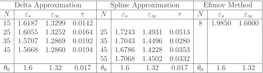
a distribution of similar characteristics to describe a CMC which is in a crystalline state. In Figure 1 we give the model fit for both PMF approximation schemes using N = 45 as well as for the modified Efimov approach withJ = 6. We see that both PMF methods obtain an excellent model fit, and similar fits were obtained for other values ofN. The model using the modified Efimov approach fits the data well except for wavenumbersk > 1350 cm−1. We
present the estimated distributions using the spline and Dirac methods in Figure 2 and the estimated scalar parameters can be found in Table 1.
6000 700 800 900 1000 1100 1200 1300 1400 0.02
0.04 0.06 0.08 0.1 0.12 0.14 0.16
k, 1/cm
Reflectance
Data Model fit (D45) Model fit (S45) Model fit (E6)
Figure 1: The model fits to the simulated data generated with a discrete distribution. The model fit using the Dirac approximation scheme is labeled as D45 and the spline approx-imation schemes as S45, where 45 is the number of nodes N, and the model fit using the modified Efimov method is labeled as E6 where J = 6 oscillators were used.
500 1000 1500
0 0.2 0.4 0.6 0.8 1
k0, 1/cm
Probability Distribution
True Distribution Estimated (D15) Estimated (D25) Estimated (D35) Estimated (D45)
500 1000 1500
0 0.2 0.4 0.6 0.8 1
k0, 1/cm
Probability Distribution
True Distribution Estimated (S25) Estimated (S35) Estimated (S45) Estimated (S55)
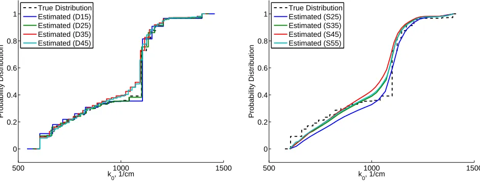
Figure 2: The estimated distributions to the simulated data using a discrete distribution using the Dirac approximation method with N = 15,25,35 and 45 nodes (left) and using the spline approximation method with N = 25,35,45 and 55 nodes (right).
The estimated distribution using the spline method is not able to replicate the large jump at k0 = 1100 cm−1, even when using as many as N = 55 nodes. However, in general, the
Delta Approximation Spline Approximation Efimov Method
N εs ε∞ τ N εs ε∞ τ N εs ε∞
15 1.6187 1.3299 0.0142 8 1.9850 1.6000
25 1.6055 1.3252 0.0164 25 1.7243 1.4931 0.0513 35 1.5707 1.2869 0.0192 35 1.7043 1.4496 0.0280 45 1.5668 1.2860 0.0194 45 1.6786 1.4228 0.0353 55 1.7068 1.4502 0.0332
θ0 1.6 1.32 0.017 θ0 1.6 1.32 0.017 θ0 1.6 1.32
Table 1: The estimated parameters using the Dirac and spline approximation methods for the discrete distribution.
Oscillator (j) Sj τj k0j σj
1 6.2021e+04 0.0060 600.22 88.37
2 1.9846e+04 0.0135 839.29 56.89
3 1.6175e+02 0.0064 839.87 119.82
4 2.7413e+04 0.0968 1103.13 14.17
5 1.7871e+05 0.0124 1123.55 19.92
6 1.3596e+04 0.0317 1207.65 17.02
Table 2: The estimated values of the intensities Sj, the relaxation times τj, the resonance
wavenumbersk0j and the standard deviationsσj for each oscillator using the modified Efimov approach, using the simulated data with a discrete distribution.
In Table 2 we give the estimated values for the individual oscillators using the modified Efimov model. We expect to see an oscillator centered near 1100 cm−1 with a narrow
broad-ening (i.e. a small standard deviation) to describe the jump discontinuity in the distribution. Indeed, we see that the 4th oscillator is centered at k04 = 1103.13 cm
−1 and has a standard
deviation ofσj = 14.17. Unexpectedly we also see that the 5th and 6th oscillators also have
a narrow broadening. Furthermore, using the Efimov approach, it is difficult to associate the oscillator directly to the size of the jump discontinuity in the distribution, one must look at the magnitude of the intensity Sj relative to the other intensities to understand the
relative “importance” of each oscillator. That is, from Table 2 we would deduce that the 5th
oscillator with an intensity on the order to 105 has more importance compared to the 3rd
oscillator which has an intensity of 102 three orders of magnitude lower.
3.1.2 Continuous distribution
In this example we consider the case where the true distribution G0 is taken as a truncated
bivariate normal distribution with corresponding probability density function g0 given by
G0(k0) =
β σ1
√
2π exp
−(k0−µ1)
2
2σ2 1
+ β
σ2
√
2π exp
−(k0−µ2)
2
2σ2 2
In the above equation, we take µ1 = 850 cm−1,µ2 = 1050 cm−1,σ1 = 70, σ2 = 60, k0 = 600
cm−1, k
0 = 1400 cm−1 and β is the normalizing constant
β−1 = Z k0
k0
1
σ1
√
2πexp
−(k0−µ1)
2
2σ2 1
+ 1
σ2
√
2πexp
−(k0−µ2)
2
2σ2 2
dk0. (3.2)
We expect that a CMC in an amorphous state would best be represented by a continuous distribution.
6000 700 800 900 1000 1100 1200 1300 1400 0.02
0.04 0.06 0.08 0.1 0.12 0.14 0.16
k, 1/cm
Reflectance
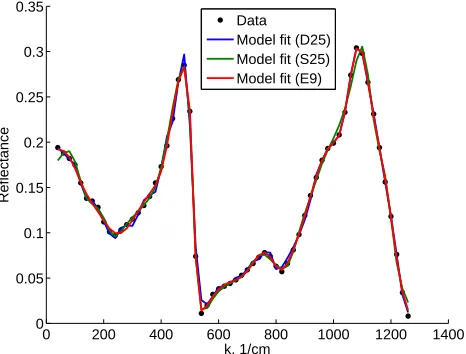
Data Model fit (D25) Model fit (S25) Model fit (E2)
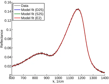
Figure 3: The model fits to the simulated data generated with a continuous distribution.
For the Dirac and spline approximation schemes the number of nodes was taken as N = 25
(labeled as D25 and S25 respectively) and for the Efimov approach we have J = 2 (labeled as E2).
Delta Approximation Spline Approximation Efimov Method
N εs ε∞ τ N εs ε∞ τ N εs ε∞
10 1.4519 1.1613 0.0101 10 1.9299 1.7017 0.0264 2 1.5747 1.3013
15 1.4107 1.1239 0.0112 15 1.5768 1.3040 0.0156 20 1.4011 1.1174 0.0116 20 1.5751 1.3074 0.0195 25 1.3909 1.1090 0.0124 25 1.5717 1.3077 0.0261
θ0 1.6 1.32 0.017 θ0 1.6 1.32 0.017 θ0 1.6 1.32
Table 3: The estimated parameters using the Dirac and spline approximation methods for the simulated data with a continuous distribution.
500 1000 1500 0
0.2 0.4 0.6 0.8 1
k0, 1/cm
Probability Distribution
True Distribution Estimated (D10) Estimated (D15) Estimated (D20) Estimated (D25)
600 700 800 900 1000 1100 1200 1300 1400
0 0.2 0.4 0.6 0.8 1
k0, 1/cm
Probability Distribution
True Distribution Estimated (S10) Estimated (S15) Estimated (S20) Estimated (S25)
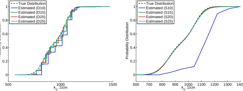
Figure 4: The estimated distributions to the simulated data using a continuous distribution using the Dirac approximation method (left) and using the spline approximation method (right). For both methods we chose the number of nodes to be N = 10,15,20 and 25.
Oscillator (j) Sj(1×10⁵) τj k0j σj
1 1.0170 0.0139 861.23 66.61
2 1.4794 0.0175 1057.06 60.07
Table 4: The estimated values of the intensities Sj, the relaxation times τj, the resonance
wavenumbersk0j and the standard deviationsσj for each oscillator using the modified Efimov approach using the simulated data with a continuous distribution.
in the approximation scheme to accurately fit the data. The Efimov approach is able to accurately fit the data with only J = 2 oscillators, which is not surprising since the true distribution is composed of two normal distributions.
From Table 3, we see that the constant parameters are more accurately estimated using the spline approximation scheme and the Efimov approach. However, again the value for τ
is difficult to estimate correctly.
In Table 4 we see that we obtain a good estimate for the relaxation time for the second oscillator, but not for the first. The resonance wavenumbers and the standard deviations for both oscillators are a good estimation of the mean and standard deviations of the bivariate normal distribution.
3.2
Inorganic glass data
3.2.1 Vitreous Silica
We first consider reflectivity data collected from Vitreous Silica in the 200 to 1350 cm−1
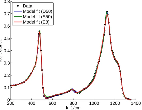
range (see Table A2 in [11]). In Figure 5 we present the model fits to the data using the
Dirac and spline approximations with N = 50 for both methods and using the modified
Efimov method with J = 8. We see that all of the methods are able to obtain a good fit to the data.
2000 400 600 800 1000 1200 1400
0.1 0.2 0.3 0.4 0.5 0.6 0.7 0.8
k, 1/cm
Reflectance
Data Model fit (D50) Model fit (S50) Model fit (E8)
Figure 5: The model fits to the Vitreous Silica data.. For the Dirac and spline approximation
schemes the number of nodes was taken as N = 50 (labeled as D50 and S50 respectively)
and for the Efimov approach we have J = 8 (labeled as E8).
0 200 400 600 800 1000 1200 1400
0 0.2 0.4 0.6 0.8 1
k0, 1/cm
Probability Distribution
Estimated (D30) Estimated (D50) Estimated (D80)
200 400 600 800 1000 1200 1400
0 0.2 0.4 0.6 0.8 1
k0, 1/cm
Probability Distribution
Estimated (S30) Estimated (S50) Estimated (S80)
Figure 6: The estimated distributions to the Vitreous Silica data using the Dirac approxi-mation method (left) and using the spline approxiapproxi-mation method (right). For both methods we chose the number of nodes to be N = 30, 50 and 80.
method has converged for a relatively low value of N. The spline method gives consistent
results for N = 50 and 80; the distribution obtained using N = 30 has the same general
characteristic shape as the other two distributions, but it is clearly an outlier. Thus, we may
assume that the spline method has not converged at N = 30, but has by N = 50. In fact,
once both methods have converged, they have converged to the same distribution. Although the estimated distribution has large jumps near k0 = 400 cm−1 and 1050 cm−1, we agin see
the surprising result that the spline approximation method is able to handle these regions of rapid change in the distribution.
Delta Approximation Spline Approximation Efimov Method
N εs ε∞ τ N εs ε∞ τ N εs ε∞
30 3.7535 2.0845 0.0398 30 3.3489 1.5553 0.1032 8 3.7530 2.1384
50 3.7183 2.0487 0.0522 50 3.7079 2.0581 0.2020 80 3.6780 2.0153 0.0564 80 3.7019 2.0675 0.1851
θ0 3.8 2.1 θ0 3.8 2.1 θ0 3.8 2.1
Table 5: The estimated parameter values using the Dirac and spline approximation methods to fit the Vitreous Silica data. The “true” parameter values θ0 are the experimental values
taken from [15].
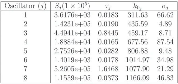
Oscillator (j) Sj(1×10⁵) τj k0j σj
1 3.6176e+03 0.0183 311.63 66.62
2 1.4231e+05 0.0190 435.59 4.89
3 4.4941e+04 0.8445 459.17 8.71
4 1.8884e+04 0.0165 677.56 87.54
5 2.7526e+04 0.0282 806.88 9.48
6 1.4019e+03 0.0178 1014.97 34.98
7 5.2605e+05 1.6468 1077.90 21.29
8 1.1559e+05 0.0373 1166.09 46.83
Table 6: The estimated values of the intensities Sj, the relaxation times τj, the resonance
wavenumbersk0j and the standard deviationsσj for each oscillator using the modified Efimov approach on the Vitreous Silica data.
In Table 5, we present the estimated parameter values using both PMF methods. Notice that the estimated values of εs and ε∞ are very similar for N = 30 , 50 and 80 using the
Dirac approximation method. However, the values forεs andε∞using the spline method do
not match the values obtained using the Dirac approximation at N = 30, but do forN = 50 and 80. Thus, again indicating that the Dirac method converges for a lower value of N than the spline method. We also see that the high and low frequency limits are well approximated by the modified Efimov method.
The estimated values of the individual oscillators using the modified Efimov method are given in Table 6. The 2nd, 3rdand 5th oscillators, centered at approximately 435, 459 and 806 cm−1, respectively, each have a very narrow broadening. The 2nd and 3rd oscillators
The 5thoscillator is present in a region where the estimated distribution does not contain a sharp jump.
3.2.2 Vitreous Germania
We next consider reflectivity data collected from Vitreous Germania in the 200 to 1350 cm−1 range (see Table A7 in [11]). In Figure 7 we present the model fit and the estimated
distributions using both the Dirac and spline methods with N = 50 and using the modified Efimov method with J = 8. Once again, we obtain very good fits to the data in all cases.
4000 500 600 700 800 900 1000 1100
0.1 0.2 0.3 0.4 0.5 0.6 0.7
k, 1/cm
Reflectance
Data Model fit (D50) Model fit (S50) Model fit (E8)
Figure 7: The model fits to the Vitreous Germania data. For the Dirac and spline
ap-proximation schemes the number of nodes was taken as N = 50 (labeled as D50 and S50
respectively) and for the Efimov approach we have J = 8 (labeled as E8).
300 400 500 600 700 800 900 1000 1100
0 0.2 0.4 0.6 0.8 1
k0, 1/cm
Probability Distribution
Estimated (D30) Estimated (D50) Estimated (D80)
400 500 600 700 800 900 1000 1100
0 0.2 0.4 0.6 0.8 1
k0, 1/cm
Probability Distribution
Estimated (S30) Estimated (S50) Estimated (S80)
Figure 8: The estimated distributions to the Vitreous Germania data using the Dirac ap-proximation method (left) and using the spline apap-proximation method (right). For both
From Figure 8 we see that each estimation using the spline method gives consistent results, and the estimation with N = 30 using the Dirac method does not match the results using N = 50 and 80. In this case, the results suggest that the spline method converges for a lower number of nodes than the Dirac method, but both methods do converge to the same distribution. This should be expected since it appears as if the estimated distribution is sufficiently smooth, and it is known [8] that the spline method will outperform the Dirac method in this case.
In Table 7 we present the estimated parameter values for both methods. This time we see that the spline method gives consistent values for εs and ε∞, whereas for N = 30, the
values estimated using the Dirac method are the outliers. The estimated values for εs and
ε∞using the modified Efimov approach are slightly higher than the estimates using the PMF
methods.
Delta Approximation Spline Approximation Efimov Method
N εs ε∞ τ N εs ε∞ τ N εs ε∞
30 2.3992 1.7707 0.0779 30 2.0034 1.3320 0.4989 8 2.1844 1.5200
50 1.8961 1.3013 0.7741 50 2.0567 1.3854 0.2581 80 1.9068 1.3435 0.6250 80 2.0254 1.3659 0.4964
Table 7: The estimated parameter values using the Dirac and spline approximation methods to fit the Vitreous Gernamia data.
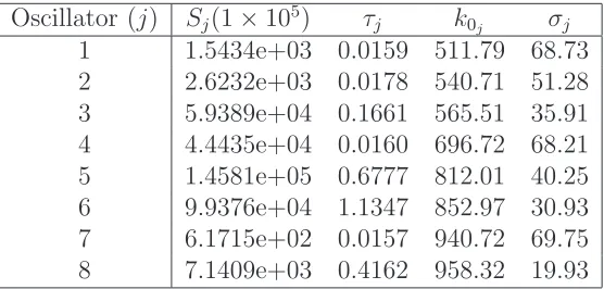
Oscillator (j) Sj(1×10⁵) τj k0j σj
1 1.5434e+03 0.0159 511.79 68.73
2 2.6232e+03 0.0178 540.71 51.28
3 5.9389e+04 0.1661 565.51 35.91
4 4.4435e+04 0.0160 696.72 68.21
5 1.4581e+05 0.6777 812.01 40.25
6 9.9376e+04 1.1347 852.97 30.93
7 6.1715e+02 0.0157 940.72 69.75
8 7.1409e+03 0.4162 958.32 19.93
Table 8: The estimated values of the intensities Sj, the relaxation times τj, the resonance
wavenumbersk0j and the standard deviationsσj for each oscillator using the modified Efimov approach on the data obtain from Vitreous Germania.
In Table 8 we present the individual oscillator estimates obtain from the modified Efimov approach. In this case we see that the only oscillator which has a somewhat narrow broad-ening is present at 958 cm−1. This oscillator has an intensity of 103, two orders of magnitude
3.2.3 Sodium Silicate
As a final consideration, we use reflectivity data collected from Sodium Silicate in the 40 to 1260 cm−1 range (see Table A3 in [11]). In Figure 9 we give the model fit to the data and
the estimated distributions using the Dirac and spline approximation schemes using N = 25
and using the modified Efimov approach with J = 9.
We see that the estimated distributions using both methods agree very well for the relatively low number of nodes, and the agreement is increased for N = 30 as is seen from Figure 10. Additionally, in Table 9 we see that the estimated values ofεs andε∞ agree well
for N = 30. Thus, it appears in this case that both the spline and Dirac approximation
methods have converged at a relatively low number of nodes. It should be noted, that for this particular data set, there were 62 data points, which is why we did not use a larger number of nodes thanN = 30. Using the modified Efimov approach, the estimated value of
ε∞ is consistent with the results using the PMF, but the value ofεs does not match.
0 200 400 600 800 1000 1200 1400
0 0.05 0.1 0.15 0.2 0.25 0.3 0.35
k, 1/cm
Reflectance
Data Model fit (D25) Model fit (S25) Model fit (E9)
Figure 9: The model fits to the Sodium Silicate data. For the Dirac and spline approximation
schemes the number of nodes was taken as N = 25 (labeled as D25 and S25 respectively)
and for the Efimov approach we have J = 9 (labeled as E9).
Delta Approximation Spline Approximation Efimov Method
N εs ε∞ τ N εs ε∞ τ N εs ε∞
25 6.3266 2.1110 0.0200 25 5.7623 1.5496 0.0269 9 7.4048 2.1179
30 5.9747 2.0939 0.0240 30 5.9068 1.9573 0.0305
Table 9: The estimated parameter values using the Dirac and spline approximation methods as compared to the Efimov method to fit the Sodium Silicate Silica data.
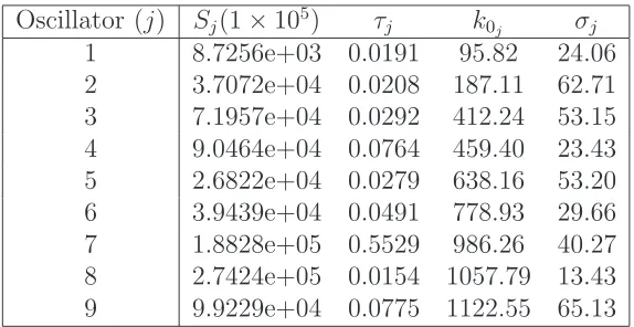
In Table 10 we present the estimation results for the oscillators using the modified Efimov approach. In this case, the oscillator with the most narrow broadening is the 8th oscillator which is centered at 1057 cm−1. This oscillator corresponds to a region of relatively gradual
0 200 400 600 800 1000 1200 1400 0
0.2 0.4 0.6 0.8 1
k0, 1/cm
Probability Distribution
Estimated (D25) Estimated (D30)
0 200 400 600 800 1000 1200 1400
0 0.2 0.4 0.6 0.8 1
k0, 1/cm
Probability Distribution
Estimated (S25) Estimated (S30)
Figure 10: The estimated distributions to the Sodium Silicate data using the Dirac approxi-mation method (left) and using the spline approxiapproxi-mation method (right). For both methods
we chose the number of nodes to be N = 25 and 30.
Oscillator (j) Sj(1×10⁵) τj k0j σj
1 8.7256e+03 0.0191 95.82 24.06
2 3.7072e+04 0.0208 187.11 62.71
3 7.1957e+04 0.0292 412.24 53.15
4 9.0464e+04 0.0764 459.40 23.43
5 2.6822e+04 0.0279 638.16 53.20
6 3.9439e+04 0.0491 778.93 29.66
7 1.8828e+05 0.5529 986.26 40.27
8 2.7424e+05 0.0154 1057.79 13.43
9 9.9229e+04 0.0775 1122.55 65.13
Table 10: The estimated values of the intensities Sj, the relaxation times τj, the resonance
4
Concluding remarks and future work
In this work we consider two contrasting methods of modeling the complex permittivity of a material in which the number of dielectric mechanisms is unknown. Using the PMF, we imposed a distribution on the resonance wavenumber and considered two approximation schemes for estimating the unknown distribution. We also considered a method which uses a convolution of Lorentz and Gaussian functions, the modified Efimov approach. We consid-ered both simulated and experimental data sets. Within the context of the PMF, it is clear that considering the model fits alone are not sufficient to determine which approximation scheme to use, since both consistently give good model fits even if the estimated distributions vary. It is not surprising that the Dirac methods are better suited to estimate a discontinuous distribution and that the spline method are better suited to handle estimating a continuous distribution. In practice of course, there in general is no prior knowledge as to the form of the unknown distribution (continuous or discontinuous). Fortunately, we have illustrated in the examples presented in this work that the spline approximation method gives reasonable estimates even for the cases where the true distribution possesses discontinuities. Thus, it is our recommendation that initially both methods should be used to do the inverse problem. Once it is established that the estimated distributions using both methods sufficiently agree, then the results obtained using the lowest number of nodes possible to achieve this agree-ment should be used. This should minimize any effects of over parameterization (see Section 3.1.1). Only after the distributions agree should the decision be made as to whether the distribution appears to obtain discontinuities. If discontinuities (or regions of relative rapid change) are present in the distribution, then the results using the Dirac method would be preferred, and the results from the spline approximation would be preferred for distributions which appear continuous in nature.
Using the modified Efimov method, we were also able to obtain very good model fits to the data for both the simulated data and the inorganic glass data. It was seen that using this approach, regions of rapid increase in the distribution will correspond to oscillators with a narrow broadening. However, one pitfall to this approach is the difficulty in ascertaining the relative “importance” of each oscillator, for which the only indication is the estimated intensity. One advantage that the PMF approach has over the modified Efimov approach is that the estimated distribution can easily be interpreted. Furthermore, there is a strong theoretical foundation for the PMF approximation schemes to converge asN → ∞(with the assumption that the density function is absolutely continuous in the case of using splines), however, there is no known sense of convergence asJ → ∞ in the Efimov approach.
Acknowledgements
This research was supported in part by the Air Force Office of Scientific Research under grant number AFOSR FA9550-12-1-0188, and in part by the US Department of Education Grad-uate Assistance in Areas of National Need (GAANN) under grant number P200A120047. The authors are gratefully to Dr. Amanda Criner and her colleagues at Wright-Patterson Air Force Base for their encouragement and insightful comments regarding this work.
References
[1] P. Baldus, M. Jansen and D. Sporn, Ceramic Fibers for Matrix Composites in High-Temperature Engine Applications, Science, 285 (1999), 699–703.
[2] H.T. Banks, A Functional Analysis Framework for Modeling, Estimation and Control
in Science and Engineering, Chapman and Hall/CRC Press, Boca Raton, FL, 2012.
[3] H.T. Banks and K.L. Bihari, Modeling and estimating uncertainty in parameter esti-mation, Inverse Problems, 17 (2001), 95-111.
[4] H. T. Banks, J. Catenacci, and S. Hu, Estimation of distributed parameters in permit-tivity models of composite dielectric materials using reflectance, CRSC–TR14–08, N. C. State University, Raleigh, NC, June, 2014; J. Inverse and Ill-posed Problems, to appear.
[5] H.T. Banks, J. Catenacci and S. Hu, Asymptotic properties of probability measure
esti-mators in a nonparametric model, SIAM/ASA Journal on Uncertainty Quantification,
to appear.
[6] H.T. Banks and N.L. Gibson, Electromagnetic inverse problems involving distributions of dielectric mechanisms and parameters, Quarterly of Applied Mathematics, 64 (2006), 749–795.
[7] H.T. Banks, S. Hu, and W.C. Thompson, Modeling and Inverse Problems in the
Pres-ence of Uncertainty, Chapman & Hall/CRC Press, Boca Raton, FL, 2014.
[8] H.T. Banks and G.A. Pinter, A probabilistic multiscale approach to hysteresis in shear wave propagation in biotissue, SIAM J. Multiscale Modeling and Simulation, 3 (2005), 395412.
[9] J.G. Blaschak and J. Fanzen, Precursor propagation in dispersive media from short-rise-time pulses at oblique incidence, Journal of the Optical Society of America A, 12 (1995), 1501-1512.
[10] A.T. Cooney, R.Y. Flattum-Riemers, and B.J. Scott, Characterization of material degra-dation in ceramic matrix composites using infrared reflectance spectroscopy, AIP Con-ference Proceedings, San Diego, California, July 18–23, 2010.
[12] A.M. Efimov, Quantitative IR spectroscopy: Applications to studying glass structure and properties, Journal of Non-Crystalline Solids, 203 (1996), 1–11.
[13] A.M. Efimov, Vibrational spectra, related properties, and structure of inorganic glasses, Journal of Non-Crystalline Solids, 253 (1999), 95–118.
[14] A.M. Efimov and E. G. Makarova, Dispersion equation for the complex dielectric con-stant of vitreous solids and dispersion analysis of their reflection spectra, Fiz. Khim. Stekla (Journal of Applied Spectroscopy), 11, (1985), 385.
[15] L. Giacomazzi and A. Pasquarello, Vibrational spectra of vitreous SiO2 and vitreous
GeO2 from first principles, Journal of Physics: Condensed Matter, 19 (2007), 112–121.
[16] S.R. Pina, L.C. Pardini, I.V. Yoshida, Carbon fiber/ceramic matrix composites: pro-cessing, oxidation and mechanical properties, Journal of Material Science, 42 (2007) 4245–4253.
[17] Yu.V. Prohorov, Convergence of random processes and limit theorems in probability theory, Theor. Prob. Appl., 1 (1956), 157–214.
[18] G. Qi, C. Zhang, H. Hu, F. Cao, S. Wang, Y. Jiang, B. Li, Crystallization behavior of three-dimensional silica fiber reinforced silicon nitride composite, Journal of Crystal Growth, 284 (2005), 293–296.
[19] H. Ohnabe, S. Masaki, M. Onozuka, K. Miyahara, T. Sasa, Potential application of
ceramic matrix composites to aero-engine components, Composites Part A: Applied
Sciences and Manufacturing, 30 (1999), 489–496.