ABSTRACT
LI, SIBO. Study on micromachined piezoelectric material and dual-layer transducers for ultrasound imaging. (Under the direction of Dr. Xiaoning Jiang).
Medical ultrasound has been widely used in cardiology, obstetrics, gynecology,
prostate evaluation, and blood vessels assessment. Advances in medical ultrasound have been
limited by difficulties in developing transducer arrays with broad bandwidth and high
sensitivity. Ultrasound arrays are preferred in advanced imaging because of the trade-offs
among resolutions, depth of field and frame rate using the single-element transducers. In
high-frequency ultrasound array development, piezoelectric materials and structures are known to
greatly influence the imaging performance. The problem encountered with the array ultrasound
for superharmonic imaging is the broad bandpass requirement for fundamental transmission
and superharmonic detection. The objective of this thesis is to investigate and evaluate novel
designs of high-frequency circular array for intravascular ultrasound and dual-frequency
collinear array for microbubble superharmonic imaging that overcome the problems associated
with conventional arrays.
High-frequency broadband (-6dB fractional bandwidth > 70%) micromachined 1-3
composites are preferred because of their superior electromechanical coupling coefficient (kt
~ 0.76) and relatively low acoustic impedance (Z ~20 MRayl). Those properties showed great
potential as an active material for transducer development. In this study, a 40-MHz
micromachined PMN-PT 1-3 composite circular array was designed, fabricated and
(radially outwards) with the pitch of 100 m was wrapped around a needle resulting in an outer
diameter of 1.7 mm. The array test showed that the center frequency was 39±2 MHz and
−6-dB fractional bandwidth was 82±6%. The insertion loss was −41 −6-dB, and crosstalk between
adjacent elements was −24 dB. A radial outward imaging testing with phantom wires (D = 50
m) was conducted. The image was in a dynamic range of 30 dB to show a penetration depth
of 6 mm by using the synthetic aperture method. The −6 dB beamwidth was estimated to be
60 m in the axial direction at 3.1 mm distance away from the probe. The results suggest that
the 40 MHz micromachined 1-3 composite circular array is promising for intravascular
ultrasound imaging applications.
Ultrasound contrast agent based superharmonic imaging is the second topic discussed
in the thesis. Based on the nonlinear responses of the microbubbles, conventional ultrasound
with a single frequency and limited bandpass cannot achieve the fundamental frequency
transmission and superharmonic detection. To meet this requirement, the development of the
array ultrasound with multi-center-frequency is proposed for the microbubbles superharmonic
imaging. The probe consists of 64 transmit elements with a center frequency of 3 MHz and
128 receiving elements with a center frequency of 15 MHz. The dimensions of the array are
18 mm in azimuth and 8 mm in elevation. The pitch is 280 m for transmitting (TX) elements
and 140 m for receiving (RX) elements. Pulse-echo test of TX/RX elements and the acoustic
field for focal beam were conducted and compared with the simulation results. Real-time
contrast imaging was carried out using a Verasonics system on a tissue-mimicking phantom.
underneath the skin of a rat. These results indicate the potential use of the co-linear array for
acoustic angiography imaging of prostate tumor and identification of regions of
© Copyright 2017 by Sibo Li
Micromachined Piezoelectric Material and Dual-layer Transducers for Ultrasound Imaging
by Sibo Li
A dissertation submitted to the Graduate Faculty of North Carolina State University
in partial fulfillment of the requirements for the degree of
Doctor of Philosophy
Mechanical Engineering
Raleigh, North Carolina
2017
APPROVED BY:
_______________________________ ______________________________ Dr. Yun Jing Dr. Marie Muller
________________________________ ________________________________ Dr. Paul A. Dayton Dr. Xiaoning Jiang
DEDICATION
BIOGRAPHY
Sibo Li received his B.S. degree in mechanical engineering from University of Science and
technology of China in 2008, his M.S. in mechanical engineering from Stevens Institute of
Technology in 2012. After that, He joined Dr. Xiaoning Jiang’s group at North Carolina State
University. His current research majored in array transducer design and fabrication for prostate
acoustic angiography, piezoelectric composite micromachined ultrasound transducers
ACKNOWLEDGMENTS
The doctoral dissertation is a result of the work of more than just the person whose name
is on it. I have been privileged to work with and be inspired by many people during the five
years to produce this research. I first want to thank Dr. Xiaoning Jiang for all of his support
and encouragement. It was extremely fortunate for me to have such a supervisor, who always
had time for me even for the last-minute tasks, and taught me so much in every aspect of
science, from experimental design to data analysis, from critical thinking to scientific writing.
I cannot have asked for a better supervisor.
I would also like to thank the members of my doctoral committee, and all of the professors
at North Carolina State University and the University of North Carolina at Chapel Hill. I want
to thank Dr. Dayton for his guidance and patience during my transducer study and imaging
research. I am very much thankful to my colleagues in Dr. Dayton’s team, Sunny Kasoji, Heath
Martin, Brooks Lindsey and Juan Rojas.
One benefit of being at NC State for five years is that I have had a chance to meet and work
with so many wonderful students and staff. I very appreciate to the former and current members
of Micro & Nano Engineering Lab, Laura, Kyungrim, Jinwook, Jianguo, Seol, Wei-Yi,
Wennbin, Jianguo, Zhuochen, Sijia, Dr. Wu, Dr. Jian, Dr. An, Dr. Berik, Shujin, Taeyang,
Huaiyu, Lu, Joseph, and Richard who always support and encourage me as a family.
Last but not least, I would like to give my special thanks to my family, my father, my
mother, and my wife for their unconditional love and support. Without their encouragement, I
TABLE OF CONTENTS
LIST OF TABLES ... xi
LIST OF FIGURES ... xii
Chapter 1 INTRODUCTION ... 1
1.1 Motivations... 1
1.1.1 High-Frequency Ultrasound... 2
1.1.2 Superharmonic Imaging ... 3
1.2 Objectives ... 4
1.3 Outline ... 5
Chapter 2 BACKGROUND ... 8
2.1 Overview of Medical Ultrasound ... 8
2.1.1 History of Ultrasound Transducers ... 8
2.1.2 Ultrasound Imaging Principles ... 11
2.2 Transducer Structures ... 13
2.2.1 Active Layer... 13
2.2.2 Matching Layer ... 16
2.2.3 Backing Layer ... 17
2.2.4 Focusing Lens ... 18
2.3 Transducer Performance ... 21
2.3.1 Axial Resolution ... 22
2.3.2 Lateral Resolution and Depth of Field ... 24
2.3.3 Imaging Contrast and the Dynamic Range ... 26
2.3.4 Electrical Impedance ... 27
2.4 Transducer Design Model ... 28
2.5 Transducer Arrays ... 35
2.5.2 Array Category... 39
2.5.3 Array Fabrication ... 41
2.6 Image Formation with Arrays ... 43
2.6.1 Time-Gain Compensation ... 43
2.6.2 Dynamic Focusing ... 44
2.6.3 Apodization ... 44
2.6.4 Synthetic Aperture ... 46
2.7 Array Design Methods ... 47
2.8 Summary ... 49
Chapter 3 HIGH-FREQUENCY MICROMACHINED SINGLE CRYSTAL 1-3 COMPOSITE ARRAY ... 50
3.1 Background ... 50
3.2 Materials Selections for High-Frequency Ultrasound ... 51
3.2.1 Lead Zirconate Titanate (PZT) ... 52
3.2.2 Piezo Polymer ... 53
3.2.3 Relaxor-PT Single Crystals... 53
3.2.4 Lead-Free Transducer Materials ... 55
3.3 Piezo-Composites Design Criteria and Fabrication Methods ... 56
3.3.1 Piezo-Composites Theory ... 56
3.3.2 Design of High-Frequency Piezo-Composites... 60
3.3.3 Composites Fabrication ... 64
3.4 Micromachined PMN-PT Single Crystal 1-3 Composite Linear Array ... 80
3.4.1 Material Design and Fabrication ... 81
3.4.2 Material Characterization... 83
3.4.3 Array Development ... 84
3.5 Summary ... 92
4.1 Introduction ... 94
4.2 Materials and Methods ... 99
4.2.1 Material Design and Fabrication ... 99
4.2.2 Transducer Design, Fabrication, and Characterization ... 100
4.2.3 Wire Phantom Imaging ... 104
4.3 Results and discussion ... 107
4.3.1 Material Characterization... 107
4.3.2 Array Characterization ... 109
4.4 Summary ... 113
Chapter 5 A DUAL-FREQUENCY CO-LINEAR ARRAY FOR ACOUSTIC ANGIOGRAPHY ... 117
5.1 Introduction ... 117
5.2 Methods and Material... 121
5.2.1 Transducer Design and Fabrication ... 121
5.2.2 Transducer Characterization ... 125
5.2.3 In-vitro Phantom Testing ... 126
5.2.4 In-vivo Imaging ... 127
5.3 Results and Discussion ... 128
5.3.1 Array Transducer Design ... 128
5.3.2 Array Transducer Prototype ... 131
5.3.3 Characterization of the Array Transducer... 132
5.3.4 In-vitro phantom testing ... 137
5.3.5 In-vivo imaging ... 141
5.4 Conclusion ... 141
Chapter 6 CONCLUSION AND FUTURE WORK ... 143
6.1 High-frequency micromachined 1-3 composites array ... 143
6.3 Future work ... 146
6.3.1 6.3.1 Prospective study of micromachined 1-3 composites ... 146
6.3.2 6.3.2 Prospective study of multi-frequency array ultrasound ... 146
LIST OF TABLES
Table 3.1 Properties of a few important piezoelectric materials used in high-frequency
transducer designs. ... 55
Table 3.2 The material parameters for the PZT-5H and Spurr epoxy used in the model calculation ... 62
Table 3.3 Summary of the key characteristics of each method ... 78
Table 3.4 Material Properties of 1-3 Composite ... 83
Table 3.5 Array design parameters and material properties ... 85
Table 4.1 Array design parameters and material properties ... 102
Table 4.2 Material properties of 1-3 composite ... 108
Table 4.3 Measured properties for the circular array. ... 109
Table 5.1 Design parameters of the co-linear array ... 122
Table 5.2 Material properties of each component of the array ... 123
LIST OF FIGURES
Figure 2.1 A brief timeline of medical ultrasound ... 10
Figure 2.2 Diagram of the transmitting wave and receiving echo. (Top) An ultrasound transducer is excited with a voltage pulse, and transmits an acoustic pulse into the tissue. (Bottom) The transducer detects the pulses reflected from the tissue. ... 11
Figure 2.3 Diagram of the enveloped receiving signal and imaging formation. (Top) The time and amplitude of the detected signals, which represent the position of the reflector and strength of the echo. (Bottom) The signal processing from the enveloped amplitude to the brightness imaging line. ... 12
Figure 2.4 Diagram of a single-element transducer ... 13
Figure 2.5 Vibration modes of different piezoelectric geometries and their associated electromechanical coupling coefficients. ... 15
Figure 2.6 The comparison of beam pattern with and without focal lens ... 18
Figure 2.7 A diagram of a planar – concave lens. All its acoustic rays must reach point B at the same time in order to achieve focusing (top), and its simplified geometry model (bottom). ... 19
Figure 2.8 Diagram of the pulse-echo response, and the length of ringing determine the pulse width, thus determine the axial resolution. ... 20
Figure 2.9 Transmit-receiving radiation pattern for a focused transducer. ... 22
Figure 2.10 Diagram of beam pattern with different f-number resulting in different lateral resolution... 23
Figure 2.11 The intensity of echoes due to reflections at different interfaces ... 25
Figure 2.12 A typical electrical impedance magnitude and phase plot for a piezoelectric plate in the thickness mode. ... 27
Figure 2.14 1-D KLM model for T-mode, Port 1 & 2 for acoustic outputs, and Port 3 for the
inputs of electrical signals ... 29
Figure 2.15 Diagram of matrices derived from KLM model representing the overall transducer ... 33
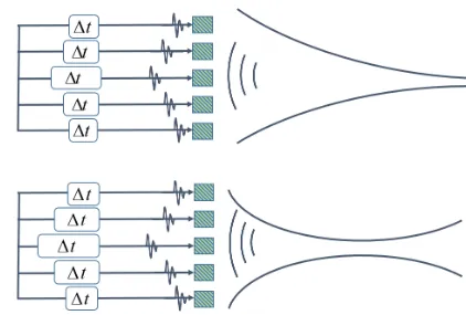
Figure 2.16 Diagram of focusing and steering an ultrasound beam with an array, (top) an array steering the ultrasound beam off the array axis; (bottom) the array focused into the tissue by applying the time delays. ... 35
Figure 2.17 The plot of the broad directivity of a λ/4 wide element and the narrow directivity of a 2λ wide element. ... 36
Figure 2.18 Plot of the radiation pattern for linear arrays excited with a continuous wave signal, showing the absence of grating lobes for a linear phased array with λ/2 element spacing, and the grating lobes at 90 degrees for a linear array with λ element spacing. ... 37
Figure 2.19 Types of transducer arrays used for medical ultrasound imaging: (a) linear array, (b) phased array, (c) 2-D array, and (d) circular array. ... 38
Figure 2.20 Beamforming of a focused scan line in an image for a linear array (left); beamforming of a focused scan line with a steering angle in a phased array (right) . ... 39
Figure 2.21 Cross-section of linear array showing the elements with the active layer and matching layers diced to separate the elements with a kerf. ... 41
Figure 2.22 The process flow of time-gain compensation (TGC) ... 42
Figure 2.23 An example of focus at different depth with different time-delay. ... 43
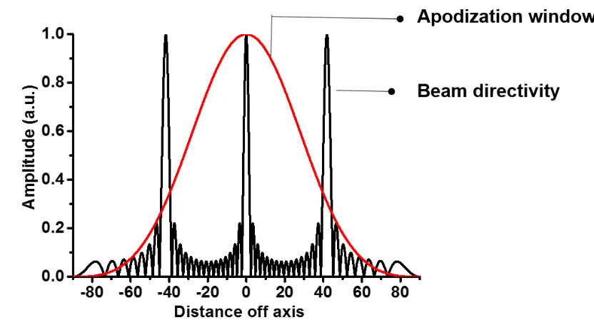
Figure 2.24 An example of apodization. ... 44
Figure 2.25 A linear array imaging with a synthetic aperture. One element is activated on transmit, while all elements are active for receive. For each successive transmit event, the next element in the array is activated, and the sequence repeated for the entire length of the array. ... 45
Figure 3.1 The schematic drawing of a 1-3 piezocomposite having a square unit cell (left) and
a concentric unit cell in a hexagonal lattice. ... 57
Figure 3.2 The coordinate system used to indicate the piezoelectric constants. ... 58
Figure 3.3 The tendency of acoustic impedance and Electro-mechanical coupling coefficient (kt) according to volume ratio increasing in composites. ... 61
Figure 3.4 Kerf dimensions of the 2-2 composite and the 1-3 composite. ... 63
Figure 3.5 Operational frequencies and their corresponding fabrication methods. ... 65
Figure 3.6 A diagram of fabrication process using dice-and-fill technique. ... 66
Figure 3.7 A diagram of the projection etch laser ablation techniques using in excimer laser. A Cr/quartz mask introduces a shadow pattern into the laser beam that is demagnified and ablated into the surface of the sample. ... 67
Figure 3.8 A diagram of the 2-2 piezoelectric composites by interdigital pair bonding. Step 1, Prepare a pair of dice ceramic sheet; Step 2, Fill the cutting grooves of of both ceramic sheets with epoxy and interdigitally insert two sheets together either by sliding or by pressing. Step 3, Cure the epoxy and lap the top and bottom surfaces. ... 69
Figure 3.9 A diagram of the 2-2 piezoelectric composites by stacking plates method. ... 71
Figure 3.10 A diagram of the 1-3 piezoelectric composites by fiber-bundling method. ... 73
Figure 3.11 A diagram of the 1-3 piezoelectric composites by molding method. ... 74
Figure 3.12 A schematic of micromachined piezo-composite process ... 76
Figure 3.13 SEM photo micrograph of a high frequency 1-3 single crystal composite fabricated by DRIE (kerf size ~5 micron meter) ... 77
Figure 3.14 The side view (left) and top view (right) of PMN-PT etching pillars ... 81
Figure 3.15 Composite under microscope view (left) and impedance spectra of free-standing 1-3 composite (right)... 84
Figure 3.17 Pulse-echo response from a KLM simulation (left), and the one from a
representative element array (right). ... 89
Figure 3.18 Measured pressure level at natural focal lateral plane from -5 mm to 5 mm (red dots) and simulated beam profile (blue line) and measured on-axis pressure level from 1 mm to 45 mm (red dots) and simulated beam curve (blue line) ... 89
Figure 3.19 Measured crosstalk for the array. ... 90
Figure 3.20 Monostatic synthetic aperture image of a wires-phantom reconstructed using a half-angle of 30°, dynamic range of the image is 30 dB and the display uses a linear gray scale for mapping ... 91
Figure 4.1 A schematic of human heart and different stages of atherosclerosis... 95
Figure 4.2 Schematic diagram of the IVUS catheter design employing (top) side-looking piezoelectric element with multiplexer, and (bottom) forward-looking CMUT array with CMOS chip ... 96
Figure 4.3 A 3-D model of 1-3 composite in COMSOL simulation. ... 98
Figure 4.4 The schematic of process for micromachined 1-3 composites ... 99
Figure 4.5 The schematic view of circular array structure ... 101
Figure 4.6 The relative positions in the wire imaging test setaup ... 105
Figure 4.7 PMN-PT 1-3 composite with conductive backing (a) top view and (b) side view. ... 106
Figure 4.8 Impedance and phase of the PMN-PT 1-3 composite; (top) Simulation results using COMSOL and (bottom) Test results. ... 107
Figure 4.9 Pulse-echo response from a KLM simulation (left), and the one from a representative element array (right). ... 110
Figure 4.11 The test result of the circular array. (Top) dielectric capacitance and loss values for each element in array; and (bottom) center frequency and bandwidth values for each element in array... 111
Figure 4.12 Measured cross-talk of the array. ... 112
Figure 4.13 Measured insertion loss. ... 112
Figure 4.14 An image of steel wires reconstructed by synthetic aperture method, with the dynamic range of 30 dB. ... 114
Figure 4.15 The beam profile of single line at 3 mm in axial direction (top) and circumferential direction (bottom). ... 115
Figure 5.1 A diagram of transrectal ultrasound (TRUS) and guided needle biopsy. (Courtesy: http://doctorbond.in) ... 117
Figure 5.2 A diagram of comparison of bubble response and tissue response. The contrast shows in the zone of higher order harmonic, resulting in the modality of superharmonic imaging. ... 119
Figure 5.3 The design of the dual-frequency dual-layer co-linear array transducer. The RX and TX elements were designed in a stack structure. An isolation layer was placed in between to minimize the aliasing echo and to get a decent bandwidth of the RX element. ... 121
Figure 5.4 The simulation of pulse-echo responses based on the KLM model for TX (top) and RX (bottom) elements. ... 127
Figure 5.5 The simulation of transducer beam profiles using the Field II program. The beam profiles were simulated with a 35-mm focus. (top) Beam profile of the low-frequency TX element without steering. (bottom) Beam profile of the high-frequency RX element without steering. ... 128
Figure 5.6 The stack structure of the dual-layer co-linear array. (top) The top view of the receiving layer (2-2 composites, with 50 m pillar and 20 m filler). (bottom) The side view of receiving layer (PZT 2-2 composites), the isolation layer (E-solder 3022), and the transmit layer (PZT ceramics)... 129
bottom view of the array transducer, including the TX element and zoom-in flex circuit (bottom-right) ... 130
Figure 5.8 Measured dielectric capacitance and loss of TX elements (a) and RX elements (b and c). ... 131
Figure 5.9 Measured electrical response of typical transducer element at TX (left) and RX (right). ... 132
Figure 5.10 Measured pulse/echo responses of typical TX (top) and RX (bottom) element and their FFT spectra. ... 134
Figure 5.11 Measured hydrophone results of TX elements acoustic mapping. The pressure mapping (unit: MPa) show two of focal depth, at 25 mm (top) and 40 mm (bottom). (Unit in color bar : MPa) ... 136
Figure 5.12 Superharmonic image of a cellulose tube filled with microbubbles in the tissue-mimicking phantom, (left) high-frequency B-mode imaging; (center) Contrast imaging without microbubbles flowing; and (right) Contrast imaging with microbubbles flowing. ... 137
Figure 5.13 The design of a tissue-mimicking phantom for the in-vitro phantom imaging (top-left); a 3D image of phantom test in different mode, high-frequency B-mode (top-right); contrast mode (without microbubble flow, bottom-left); and contrast mode (with bubble flow, bottom-right) ... 138
Figure 5.14 The experiment setup of the rat imaging and results. (top-left) The imaging setup (before the probe attached to the rat skin); (top-right) The B-mode imaging of the rat, which imaging plane was also adopted for the contrast imaging; (bottom-left) The contrast imaging without microbubbles flow; and (bottom-right) The contrast imaging with microbubbles flow. (unit: dB) ... 139
Chapter 1
INTRODUCTION
1.1 Motivations
Medical ultrasound has been one of the mainstream diagnostic modalities, which are
widely used in cardiology, obstetrics, gynecology, prostate evaluation, and blood vessels
assessment [1, 2]. The widespread usage of the ultrasound benefits from a number of unique
characteristics, which include safety (non-ionizing radiation), real-time
(direct/non-reconstructive imaging), high resolution (sub-millimeter to millimeter range for commercial
ultrasound), portability and low cost [3]. The imaging quality of ultrasound greatly relies on
the transducer performance. According to the given applications, the ultrasound transducers
used in most conventional diagnostic systems operate in the range of 1-25 MHz, which
corresponds the resolution of images on the order of 0.3-3 mm [4].
In order to further enhance ultrasound diagnostic capability, transducer studies aim to
improve the imaging performance and to expand the possible applications of medical
ultrasound [3]. In the past decades, the transducer research topics included the piezoelectric
material study [5] and transducer structure research to meet certain imaging criteria [6]. More
recently, two of active areas in medical ultrasound are the high-frequency ultrasound (>30
MHz) [7] and contrast agent based superharmonic imaging [8]. As an example of
high-frequency ultrasound, intravascular ultrasound (IVUS) imaging provides the information of
lumens, vessels, and plaque assessment. The image resolution is required to reach <100 μm,
are available by Visualsonics [9], there does not exist a high-frequency (>30 MHz) imaging
array customized for the IVUS. The first part of the thesis is addressed on the development of
a high-frequency circular array for IVUS imaging. The contrast agent, such as microbubbles,
exhibits the non-linear acoustic responses, which enable a superharmonic imaging for the
vasculature evaluation. However, conventional ultrasound with single frequency and limited
bandpass does not meet the criteria of fundamental frequency transmission and superharmonic
detection. In the second part of this thesis, it was focused on the development of dual-frequency
collinear array ultrasound to overcome this broad-bandpass challenge.
1.1.1 High-Frequency Ultrasound
High-frequency ultrasound imaging has many clinical applications because of its improved
image resolution [7]. The performance of high-frequency transducers is greatly influenced by
the properties of the piezoelectric material used in piezoelectric transducers [10]. One of the
most promising frontiers in transducer technology is the development of piezoelectric
composite materials due to their high coupling coefficient and low acoustic impedance.
Conventionally, there exist some techniques available for fabrication of piezo-polymer
composites. The most common of these is the “dice-and-fill” technique which a mechanical
dicing saw is used to cut kerfs into a piece of piezoelectric material, which are subsequently
backfilled with the epoxy. Unfortunately, this technique is problematic when considering the
small feature sizes required for high-frequency transducer operation. Recent innovation in
fabrication technology has allowed the preparation of Pb(Mg1/3Nb2/3)O3-PbTiO3 (PMN-PT)
study, the micromachining based technique is introduced and selected for the high-frequency
composite preparation.
Intravascular ultrasound (IVUS) imaging is a catheter-based system that allows physicians
to acquire images of diseased vessels from inside the artery, and recently the technique evolved
from an experimental technique to a clinical standard [13]. It provides the information and
details of lumen and vessel size, plaque area and volume, the extent and severity of disease are
frequently reflected by the echoes in ultrasound imaging. The IVUS image relies on the
ultrasound transducers performance, especially the sensitivity and resolution. To overcome the
constraints of the fixed depth-of-field and frame rate of single-element transducer based IVUS
imaging system, IVUS arrays are desirable for their beam steering, sub-aperture firing, and
higher frame rates. In 1997, a circular array of 20 MHz was developed by Volcano (Volcano
Corp., San Diego, CA) for IVUS imaging which was at the upper limit of conventional
frequencies [14]. The 3.5 French 20 MHz imaging catheters consist of 64 elements with ~50
µm pitch, integrated with five ASIC chips. To date, the high-frequency 1-3 composite (> 20
MHz) circular array has not yet been developed for IVUS imaging with enhanced performance.
In the thesis, a 40-MHz micromachined PMN-PT 1-3 composite circular array was designed,
fabricated and characterized for IVUS applications. A radial outward imaging with phantom
wires was conducted to show a gray image by using the synthetic aperture method.
1.1.2 Superharmonic Imaging
Ultrasound contrast agent based superharmonic imaging is the second topic discussed in
cancer research revealed that, during the expansion of the tumor, new blood vessels would
form from pre-existing structures surrounding the tumor in the angiogenic process.
Angiogenesis is a well-known hallmark of cancer and is characterized by increased vascular
density, vascular tortuosity, vascular malformations, and corresponding changes in blood flow
[15]. In this way, the assessment of cancer cell can be improved by imaging the vasculature.
Ultrasound contrast agents, comprising micron-sized, gas-filled microbubbles are used to
inject into the bloodstream and circulate through the vasculature [6]. When excited by an
external acoustic pulse, microbubbles oscillate non-linearly, producing waves with harmonic
waves in addition to the fundamental frequency [8]. Therefore, the vascular structure can be
mapped by capturing the harmonic signal from the flowing microbubbles, known as “acoustic
angiography” [16]. However, based on the nonlinear responses of the microbubbles,
conventional ultrasound with single frequency and limited bandpass cannot achieve the
fundamental frequency transmission and superharmonic detection. To meet this requirement,
the development of the array ultrasound with multi-center-frequency is proposed for the
microbubbles superharmonic imaging. The research is targeted for a specific application,
prostate cancer [17].
1.2 Objectives
For the high-frequency ultrasound study, although many works have been done on the array
ultrasound and micromachined high-frequency single element transducer, currently there is no
ultrasound probe available for the micromachined single crystal 1-3 composites circular array.
proposed to develop a micromachined single crystal 1-3 composite array. The specific goals
of this study are
1. To design and develop the high-frequency 1-D arrays (linear array and circular array,
respectively);
2. To develop a customized synthetic aperture imaging method for the fabricated array
ultrasound;
3. To perform the imaging testing, and demonstrate the capabilities in the image results.
For the study of the array ultrasound for superharmonic imaging, a dual-frequency array
for prostate imaging is proposed. To excite the microbubbles and meanwhile detect the
harmonic signals, the transmit array and receiving array were designed independently
meanwhile share the same acoustic aperture. A stack structure is selected, and an acoustic
isolation layer is added to separate the interference of those two layers. The objectives of this
research include:
1. To design and develop a co-linear dual-frequency array for prostate imaging;
2. To validate the idea of the acoustic angiography, and demonstrate the capabilities in the
image results.
1.3 Outline
This dissertation includes topics of the background of ultrasound, micromachined 1-3
composites 1-D array (Chapter 3 and 4) and co-linear dual-frequency array for prostate
acoustic angiography (Chapter 5). Although arrays are designed for two different applications,
typical array study follows the sequence including piezo material selection and preparation,
the design of the array element, acoustic design of the array aperture, transducer fabrication,
transducer characterization, and image testing. The rest of this dissertation is organized as
follows:
In Chapter 2, the background and approaches to the array ultrasound investigation are
described. An overview of the propagation of waves within a transducer, a summary of array
category and its imaging method are given. The modeling techniques used to evaluate the
performance of array designs are also described.
Chapter 3 and 4 cover the topics of the micromachined 1-3 composites and high-frequency
1-D array ultrasound. In Chapter 3, a brief review of piezoelectric material for the
high-frequency transducer is given, followed by the principle of 1-3 composites design. The
analytical method and finite element method are introduced as well. The fabrication process of
micromachined single crystal PMN-PT/epoxy 1-3 composites is presented. With the fabricated
material, a high-frequency flat array is developed to evaluate the performance.
The main theme of Chapter 4 is the development of a high-frequency circular array targeted
for the intravascular ultrasound imaging. A 50-element 40 MHz circular array transducer
(radially outwards) with the pitch of 100 μm is developed in an outer diameter of 1.7 mm. A
radial outward imaging testing with phantom wires (D = 50 μm) is conducted. A customized
synthetic aperture method is developed for such circular array. The results suggest that the
micromachined 1-3 composite circular array is promising for intravascular ultrasound imaging
Chapter 5 demonstrates a co-linear dual-frequency for prostate acoustic angiography. A
brief background of prostate cancer is presented. The probe consists of 64 transmitting
elements with a center frequency of 3 MHz and 128 receiving elements with a center frequency
of 15 MHz. The dimensions of the array are 18 mm in azimuth and 8 mm in elevation. The
pitch is 280 μm for transmitting (TX) elements and 140 μm for receiving (RX) elements.
Real-time contrast imaging is carried out using a Verasonics system on a tissue-mimicking phantom.
The in-vivo animal imaging demonstrated the ability to detect individual vessels underneath
the skin of a rat. These results indicate the potential use of the co-linear array for acoustic
angiography imaging of prostate tumor and identification of regions of neovascularization for
the guidance of prostate biopsies.
Finally, Chapter 6 summarizes the research findings, followed by suggestions for the future
Chapter 2
BACKGROUND
2.1 Overview of Medical Ultrasound
Ultrasound is a widespread tool for medical diagnosis. It is useful and popular as an
imaging modality due to the absence of ionizing radiation, and inexpensive procedure
compared to computed tomography (CT), magnetic resonance imaging (MRI), and
positron-emission tomography (PET). Another major advantage of ultrasound imaging is that the
images are produced in real-time, which is critical to the clinical surgery. Ultrasound, in
general, is used to image the soft tissues, which the uses include obstetrics, cardiology,
dermatology, and ophthalmology [3]. One of the most popular applications of ultrasound is in
the obstetrics, for imaging and measuring the growth of the baby in utero [18]. The real-time
nature of ultrasound imaging is indispensable in cardiology for a proper examination of a
beating heart. Ultrasound is also used for the detection of the blood flow by detecting the
Doppler shift of the reflected signals, known as Doppler ultrasound [3]. Ultrasound is also
available in oncology for the detection and evaluation of tumors, particularly for evaluating
the progress of therapy [15].
2.1.1 History of Ultrasound Transducers
Medical ultrasound imaging stems from the sonar technology, which uses ultrasound
frequencies between 100 KHz and 1 MHz to detect the targets deep in the sea [19]. Sonar was
used to produce and detect the acoustic pulse. The concept of sonar was later applied to
imaging the human tissues by increasing the ultrasound frequencies above 1 MHz. Imaging
with ultrasound was first demonstrated to be a useful clinical tool in the early 1950’s by Wild
and Reid, who created the first two-dimensional images of soft tissues [20]. The first
ultrasound systems used a transducer that was scanned mechanically across the body to build
up a two-dimensional (2-D) image slowly. Later in 1970, the development of linear arrays and
electronic beamforming made real-time 2D image possible [21]. The development of digital
electronic beamforming in the 1980’s resulted in improved image quality and flexibility in
scanning [3]. Ultrasound is now used in almost every area of biology and medicine, and is used
in about one-third of all diagnostic imaging procedures [3, 22]. The ultrasound transducers
used in most diagnostic imaging systems operate in the range of 1-25 MHz, which corresponds
the resolution on the order of 0.3-3 mm [4].
From the 1990s to 2000s, micromachining techniques started to play a role in ultrasound
transducer, and different types of devices were developed. One of them is called CMUT,
namely capacitive micromachined ultrasonic transducer [23]. Instead of piezoelectricity,
CMUT converts the energy through the change in capacitance. By taking advantage of
micromachined fabrication, a cavity is formed in a silicon substrate, and a thin layer suspended
on the top of the cavity as a membrane. If an AC signal is applied across the biased electrodes,
the vibrating membrane will produce ultrasonic waves into the medium. If the acoustic wave
propagates across the membrane, it will generate an alternating signal as the capacitance
changes. Due to the membrane structure and low acoustic impedance of the air, CMUT shows
Because of its broad bandwidth, it could be used in second-harmonic imaging. Also some
experiments have been performed to use CMUTs as hydrophones. In 2002, Oralkan et al. first
developed a 3 MHz 1-D phased CMUT array for ultrasound imaging. The echo signals from
the target wires presented an 80% fractional bandwidth.
Piezoelectric Micromachined Ultrasonic Transducers (PMUT) is another alternative to the
conventional transducer, which is also based on the micromachining techniques [24]. Unlike
bulk piezoelectric transducers which use the thickness-mode vibration, PMUT is based on the
flexural motion of a thin membrane coupled with a piezoelectric thin film, such as PVDF and
PZT [25]. In comparison with bulk piezoelectric ultrasound transducers, PMUT offer
advantages such as increased bandwidth, flexible geometries, and good acoustic match with
medium. Besides the medical imaging, PMUT is also widely used in the fingerprint sensing
[26].
In addition to the piezoelectric effect and the capacitance based charge effect, laser induced
thermal expansion was used for high power ultrasound transducer [27]. In the laser ultrasound,
the light-sensitive absorber receives pulsed laser energy, leading to a transient thermal
expansion, generating an ultrasound wave propagating into the medium. Carbon-based
carbon candle soot [31, 32] exhibit high efficiency of light absorption and high heat transfer
rate, thus considered as light absorber material. The research in this area is active on the way
to the cavitation and drug release study [33, 34]. Based on the review of medical ultrasound
and its transducers, a chart of the timeline is summarized in Figure 2.1.
2.1.2 Ultrasound Imaging Principles
Generally, ultrasound imaging is based on echo-ranging techniques (Figure 2.2). The main
part of a transducer is a piezoelectric plate that can vibrate at a given frequency. When the
transducer is excited with a short voltage pulse, it creates a short, broadband acoustic wave
into the target medium. The wavelength λ of the propagating pulse can be expressed as follow:
v f
(2.1)
where v is the speed of sound in the tissue and f is the pulse frequency. The ultrasound energy
arrives back to the transducer mainly by the specular reflections from the tissue interfaces [3].
The reflection of the ultrasound occurs at the change in acoustic impedance, which is the basis
of ultrasound imaging. The acoustic impedance of a material Z is the product of the density ρ
and the speed of sound in the material v, as given by the following expression:
.
Z
v (2.2)The unit of acoustic impedance is the MRayl (106 kg/m2-s). Water has an acoustic impedance of 1.5 MRayl, and the acoustic impedance of soft tissue varies between 1.4 and 1.7 MRayl
[35]. The ultrasound echo is detected by the piezoelectric transducer and converted into
electrical signals (Figure 2.3). The time that echo arrives back to the transducer is determined
by the distance to the reflecting surface and the speed of sound in the tissue, which is
approximately 1500 m/s. The brightness corresponding the amplitude of the echo depends on
the mismatch of the acoustic impedance at the boundary. In this way, time-to-distance and
amplitude-to-boundary correlations were built up to express in the imaging information, which
an image line is noted as an “A-line”, where A is noted as “Amplitude”.
2.2 Transducer Structures
The ultrasound transducer is the core of the imaging system. The design of the transducer
largely determines the quality of the ultrasound image. Although the design of transducer
varies a lot based on the different requests, the constituent element is similar. A typical
single-element transducer is shown in Figure 2.4. The main structures from bottom to top are the
backing layer, active layer, matching layer, and an optional focusing lens. The transducer is
packaged in a grounded housing for the electric shielding and protection.
2.2.1 Active Layer
The heart of the transducer is the active layer, which converts mechanical energy to
electrical energy and vice versa, which is usually a piece of piezoelectric material. The name
of “piezoelectricity” is taken from the word “piezo” meaning “to press” in Greek. The most
common piezoelectric material currently used in medical ultrasound transducers are ceramics,
in particular, lead zirconate titanate, known as PZT. In recent years, with the development of
relaxor-PT single crystal, PMN-PT and its piezoelectric composites obtain much attention in
the research area, and rapidly became popular in the high-end transducer probe [5]. The study
of the piezoelectric material and related composite design are also the interest of
high-frequency ultrasound research. The detail of this part will be discussed in Chapter 3.
When a voltage pulse is applied between electrodes on the front and the back surfaces of
the piezoelectric plate, the electric pulse is converted into a mechanical expansion-contraction
resonance in its thickness dimension. This creates the acoustic pressure pulse that travels into
the tissue. When the echo wave propagates back to the piezoelectric plate, the pressure from
the acoustic pulse produces a voltage signal that can be measured. The resonance of the plate
is related to the thickness which corresponds to the half wavelength. For a given material, a
thinner substrate operates at a higher frequency. For example, a PZT plate in a transducer
operating at 5 MHz is approximately 400 μm thick.
The elastic, piezoelectric, and electrical properties of the piezoelectric material largely
determine the sensitivity of a transducer and the quality of an image [36, 37]. For
piezoelectricity, the constitutive equations for the piezoelectric materials can be expressed as
E
i ik k ij j
T
j ij i jl l
S s T d E
D d T E
(2.3)
where S, T, E, D denote the strain, stress, electric field and electric displacement, respectively.
the subscripts i, k = 1, 2, 3, 4, 5 and 6 and j, l = 1, 2 and 3. The superscript E stands for the
constant electric field condition while T means the constant stress condition. The efficiency of
the material to convert one form of energy into another is characterized by its
electromechanical coupling coefficient,
stored mechanical energy input electrical y k
energ
(2.4)
The electromechanical coupling coefficient is related not only to the material properties,
but also to the material geometries (Figure 2.5) [38, 39]. For a tall element with the sides of
the square cross-section much smaller than the height (thickness to width aspect ratio > 3), the
electromechanical coupling coefficient is denoted as k33. For a long and thin vertical plate, the
vibration mode is considered sliver mode (thickness to width aspect ratio > 3), and the
electromechanical coupling coefficient is denoted as k’33. For a disc element with the thickness
much smaller than the diameter (aspect ratio< 0.1), the electromechanical coupling coefficient
is named as kt. Due to the clamping effect of the thickness vibration mode, less electric energy
can be converted into the mechanical output, leading to a kt smaller than k’33 and k33 given the
same piezoelectric material. On the other hand, when an oscillating electric field is applied
upon a dielectric material, the electric polarization will switch itself in accordance to the
electric excitation. There always exist a delay between the excitation and the response, leading
to a dielectric loss. The dielectric loss could transform the electric energy into heat, thus
increasing the temperature of the piezoelectric material. Overheating could deteriorate the
performance of piezoelectric transducer. Hence piezoelectric materials with low dielectric loss
are preferred for the ultrasound applications. Apart from the piezoelectricity, the plate should
also have an acoustic impedance close to the acoustic impedance of tissue for efficient
transmission of the pulse to and from the tissue. While the piezoelectric plate used in
transducers have good piezoelectric and electric properties, they exhibit high acoustic
impedance (~30 MRayl) compared to tissue (~1.5 MRayl). The large acoustic mismatch may
violate the energy transmission, and the imaging sensitivity is suppressed. As a result, the
active layer alone is not good enough to acquire high quality image, and hence, backing layer
and matching layer are necessary to ensure the energy transmission and minimize the ringing
noise.
2.2.2 Matching Layer
Ideally, the acoustic impedance of piezoelectric layer should be close to the one of tissue
in order to allow the efficient transmission to and from the tissue. As mentioned above, there
energy is reflected and lost at the interface. A quarter wavelength thick matching layer is
introduced to provide the acoustic matching between the active layer and the tissue, similar to
the function of an anti-reflective coating used on an optical lens. For (2.5)a transducer with a
single matching layer, its acoustic impedance follows the equation given below [4]:
matching tissue piezo
Z Z Z (2.6)
where Zmatching, Zpiezo, and Ztissue are the acoustical impedance of matching material,
piezoelectric material and tissue, respectively. The effect of matching layer is the full energy
transmission at center frequency ideally, and an improvement in element bandwidth. Further
improvement in bandwidth can be achieved by using multiple matching layers. Searching
material with impedances of the correct magnitude is difficult. Thus, loading powders
(Alumina, Al2O3 powders) into epoxies are commonly used to form matching material, of
which the acoustic impedance can be adjusted by the percentage of loaded powder to meet the
design requirements of transducers.
2.2.3 Backing Layer
The energy generated in the transducer can radiate in both the forward direction and the
reverse direction. The purpose of the matching layer is to encourage energy to be propagated
in the forward direction with low loss. The backing layer is the opposite, which is designed to
attenuate the signal from the back surface of the piezoelectric layer, as well as reduce ringing.
Ringing is caused by energy resonating within the piezoelectric layer, and so it can be reduced
For the energy transmitted into the backing layer, an acoustically lossy material is always
preferred to mount on the back of piezoelectric layer to damp out the energy [40]. If the
attenuation of the material is sufficiently large, no reflections from the back surface of backing
layer can be found. Otherwise, it could cause some noise signals in imaging.
To minimize the ringing effect, the acoustic impedance of backing layer can be matched
to the piezoelectric material. However, as a result, half of the energy will be transferred into
the backing layer and then lost. A very short pulse could be obtained, but with a very low
amplitude. Thus compromise is always taken between sensitivity and bandwidth. Therefore,
the acoustic impedance of backing layer is usually lower than the one of the piezoelectric layer
in order to improve sensitivity. The epoxies loaded with fine powders such as tungsten are
commonly used as backing materials to increase the acoustic impedance. Usually, the thickness
of backing is at 10 wavelengths, and the acoustic impedance varies from 5 Mrayl to 14 Mrayl
according to different applications [40, 41].
2.2.4 Focusing Lens
Single-element transducers are usually equipped with a lens to focus the ultrasound beam
along the axis (Figure 2.6). This is important since the width of the ultrasound beam determines
the spatial resolution of the ultrasound system in the direction perpendicular to the propagation
direction. If a lens is used, the lens material must have an acoustic impedance matched to the
tissue but have a different speed of sound so that the acoustic signals emitted at the center of
the transducer are delayed relative to those emitted at the outer edges. The delays introduced
across the transducer face produce a concave wave front that is focused at a certain depth in
the tissue [4, 42].
Figure 2.7 A diagram of a planar – concave lens. All its acoustic rays must reach point B at the same time in order to achieve focusing (top), and its simplified geometry model
The designs of acoustic lenses share the same principles with optical lens, the Snell’s law
[43]. For small incident angles ( < 20o) we can make the approximation sin . Thus Snell’s law can be written as
1 1 1 2
2 2 2 1
sin sin
c n
c n
(2.7)
where 1 and 2 denote the incident angle and departure angle, c1 and c2 denote the speed of
two materials, and n1, n2 denote the refractive index. While for electromagnetic waves the
propagation speed in vacuum serves as a reference, there is no reference speed for sound. Thus
the acoustic refractive index is defined as reciprocal value of the medium’s sound speed.
1
n c
(2.8)
For example as a plane wave to a focal beam (Figure 2.7), in order to achieve focusing at point
B, the time required for the ray from left to the focal point should be a constant. Consequently,
the condition for focusing can be simply written as
1 1 2 2
n d n d const (2.9)
To find a suitable lens geometry for focusing planar waves, it was suggested to use a type of
geometrical shapes called “Conics” [43]. The property of this geometry can be described as
r
const
MP (2.10)
where r is the curvature radius at point P, and MP denotes the distance of sound traveling in
the lens. The formula can be utilized for designing a planar-concave lens. If the coordinate
system’s point of origin is selected at the “geometry focal point” of the parabola curve, the
radius of the curve can be given by
( )
1 cos( ) D
r
(2.11)
where D is the distance from the point of origin to the Directrix line, and ɛ is called the
“eccentricity” of the curve. Based on this method, with given focal distance and material
parameter, the design of the focal lens can be obtained.
2.3 Transducer Performance
The quality of an image is dependent on the axial resolution, lateral resolution and contrast
electrical impedance of the transducer. These specifications are determined by the transducer
design and geometry [44].
2.3.1 Axial Resolution
The axial resolution is the closest distance two objects can be recognized along with an
image line and be detected separately. The axial resolution is determined by the time duration
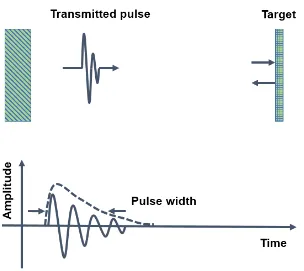
of the pulse-echo response of the transducer [3]. Figure 2.8 is a diagram of the pulse-echo
response measurement. The pulse transmitted by the transducer is reflected from a target, and
the envelope of the detected signal is calculated. The pulse length T is the temporal width of
the envelope at half the maximum (-6 dB width). Two point targets will appear as individual
reflectors in an image if the reflected signals are separated by a time greater than T. The
corresponding spatial axial resolution Raxial is given by the following equation:
1 , 2
axial
R vT (2.12)
where v is the speed of sound in the tissue. A shorter pulse provides a better axial resolution.
The limit of the axial resolution is half of the wavelength in the tissue. The axial resolution of
a transducer can be improved by using more matching layers and a backing layer with an
acoustic impedance closer to that of the piezoelectric substrate to produce a shorter pulse, or
by increasing the frequency of the pulse. The transducer should be designed so that the
pulse-echo response is as short and as broadband as possible while maintaining the sensitivity
required for the imaging application. A typical pulse has 2-3 cycles.
2.3.2 Lateral Resolution and Depth of Field
The lateral resolution of a transducer is the minimum distance between two targets can be
differentiated on the plane parallel to the transducer face. The lateral resolution is evaluated
using the radiation pattern of the transducer. The radiation pattern is the shape of the ultrasound
beam formed by a transducer. The two-way (transmit- receive) radiation pattern is measured
by scanning a point target at a fixed depth across the face of the transducer and plotting the
peak amplitude of the received signal as a function of the position of the point target. The
one-way radiation pattern is the measurement of the beam amplitude in the field of the transducer.
Because of the reciprocity of the propagation of sound waves, the one-way radiation pattern is
also the spatial response of a transducer to the signal emitted from a point source in the field.
A typical two-way radiation pattern for a focused transducer is shown in Figure 2.9. The lateral
resolution is determined by the width of the ultrasound beam, and is usually defined as the full
width at half maximum, or -6 dB width. The lateral resolution RL is given by the following
equation for a focused transducer [3]:
,
L r
R f number
D
(2.13)
where λ is the ultrasound wavelength in the tissue and the f-number is the ratio of the focal
distance r to the transducer aperture D. The lateral resolution can be improved by reducing the
focal distance of the transducer, increasing the aperture of the array, and by increasing the
The effect of aperture and focal distance on the radiation pattern is illustrated in Figure
2.10 for three transducers with different geometries. For a focused transducer, the depth of
field (DOF) is given by the following equation [45]:
2 2
8 ( ) 1 8
/ 2
DOF f number f number
D
(2.14)
Therefore, the depth of field improves with larger f-numbers and smaller apertures. As
demonstrated with the formula and the figure, there is a trade-off between resolution and depth
of field.
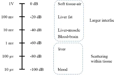
2.3.3 Imaging Contrast and the Dynamic Range
When an ultrasound pulse arrives at an interface, the reflected intensity depends on the
material mismatch and the size at the boundary. For instance, when the sound reaches the
boundary between rib bone and tissue, the reflected echo might have the same order of incident
wave. If the acoustic wave passes through a tissue-tissue gap, and the boundary size is at the
order of incident wavelength, the amplitude of the reflection could be very weak. Hence, the
range of echo amplitudes detected from different targets is very large. Figure 2.11 shows the
relative voltages and decibel scale produced by typical echoes from different target boundaries
[42].
The capability to show the imaging contrast relies on the sensitivity of the transducer and
beam pattern applied on the medium. Transducers with good sensitivity stem from the
piezoelectric material and matching/backing layer design. The beam pattern is effected by the
operating frequency and the focal performance of the transducer. A good ultrasound probe
usually can offer a dynamic range of 100 dB to differentiate the targets including large
interfaces and weak scatters. Ultrasound images are typically displayed a dynamic range of a
2.3.4 Electrical Impedance
For a piezoelectric material, the electrical behavior and mechanical behavior are coupled.
Therefore the electrical impedance can be used to identify the mechanical resonance modes of
the transducer. The complex impedance is a function of the sweeping frequency, which the
magnitude shows a valley peak corresponding to the resonance and a peak corresponding to
the anti-resonance. Figure 2.12 shows the impedance magnitude and phase spectra of a
piezoelectric plate resonating in its thickness mode. If the width or length dimensions of the
substrate are close to the thickness dimension, a second, unwanted, resonance peak would
appear in the impedance spectrum within the frequency range of interest. The unwanted
resonance reduces the sensitivity of the desired thickness-mode resonance. Therefore, the
width-to-thickness (or length-to-thickness) aspect ratio for a transducer substrate should be
better than 0.4 for a tall, thin pillar, or 2 for a wide, flat plate to operate only in its thickness
mode over a wide range of frequencies [45, 46]. The matching and backing layers dampen the
resonance, giving a broader, flatter electrical impedance amplitude and phase. The impedance
spectrum can, therefore, be used as an indication of the transducer bandwidth.
The transducer should have an electrical impedance magnitude comparable to the receive
circuitry to efficiently drive the receive electronics through the transmission cables [47].
Usually, the characteristic electrical impedance of the transmission cables is limited to 50 -
100 Ohms, the electrical impedance of the transducer should be in the same range to avoid
reflections of the signal in the cable. The small transducer elements in an array can have large
electrical impedance because the electrical impedance magnitude is inversely proportional to
the transducer area. The electrical impedance is also inversely proportional to the dielectric
constants of the transducer substrate, so the piezoelectric material can be chosen to compensate
for the transducer size; a small transducer requires a substrate with a large dielectric constant.
2.4 Transducer Design Model
In the transducer design, the structure can be expressed by a 1-D equivalent circuit model.
The analytical solutions of the model can be obtained and altered by putting different material
parameters. To correlate the acoustic and electrical parameters by using the
electrical analogy, Mason in 1964 for the first time derived the models for piezoelectric
resonator corresponding to various 1-D vibration modes [48], which is named as Mason model.
A further step based on Mason model was made by Kirmholtz, Leedom and Matthaei in 1970
by using the transmission lines [49]. This “KLM” model is named after the initials of the
authors, shows exactly same solutions to Mason model in various vibration modes but with
several advantages for design part [50].
As the most applicable medical transducer such as the single-element is the
thickness-mode vibration. A piezoelectric transducer can be treated as a three-port network system
(Figure 2.13). The electrical port represents the electrical connection between
driving/receiving circuits and transducer. The block represents the piezoelectric resonator. The
front and back acoustic port denote the front and rear surface of the piezoelectric resonator,
respectively. The backing and matching layer or fluid load can be connected to both acoustic
ports mechanically by using the acoustical-electrical analogy into the equivalent circuit. If the
acoustic ports are short-circuited, the network represents a free resonator.
In Figure 2.14, an artificial acoustic center is created by splitting the piezoelectric resonator
into halves in the thickness direction; each part with a thickness of d/2 is represented by an
acoustic transmission line. This portion allows the analysis of the two acoustic ports separately
to improve transducer design as one of the main advantages of KLM model. In the figure, V3,
I3 relates to the input voltage and current respectively; V1&2 and I1&2 are the forces and velocity
at acoustic outputs. Port 1 for acoustic back surface will be used to represent forward
transmission into fluid or body, while Port 2 for the acoustic front surface is for acoustic
backing. In order to complete the model, it is also necessary to include the acoustic impedance
of three ports, Z0, Z1, and Z3. For the piezoelectric plate, we also need to know the thickness d,
the area of the crystal A, the piezoelectric pressure constant h. The values for the piezoelectric
material are 0 0 1 2 0 0 sin cos 2 2 Z cA A C d h d X Z c Z d ec h c (2.15)
where ε is the permittivity of the piezoelectric under no voltage. The input impedance of the
piezoelectric transducer can be expressed as
_ 1 2
0
1 a
in KLM
Z
Z jX
j C
(2.16)
1 2 1 2 L L a L L Z Z Z Z Z
(2.17)
where 1,2 0 1,2 0 0 1,2 tan 2 tan 2 L d Z jZ c Z Z d Z jZ c (2.18)
Based on the equations above, the total input impedance for the KLM model can be
achieved. For the transducer design, the study is focused on the fundamental resonance
frequency ω = ω0 = cπ/d. As a result, the equations can be simplified as
2 1 2 0 0 0 2 0 1 1 2 0 2 2 2 0 1 2
_ 1 2
0 1 2 1 L L a a in KLM h X Z Z h Z Z Z Z Z Z Z Z Z Z Z Z jX j C (2.19)
With a given voltage excitation V3, the pressure radiated by the transducer can be analyzed.
With the analogy in transmission line, the particle velocity can be considered as the current I.
The particle velocities inside of the crystal are denoted by vF B,
, where the F subscript indicates
backward-traveling waves propagating towards interface, and the denote waves in the right and left half
of the crystal respectively. For the back and front half, we have
/ 2 / 2 3
/ 2 / 2 3 0 0 jkd jkd B B jkd jkd F F I
v e v e
I
v e v e
(2.20)
where k is the wave number in the crystal. However, from transmission line theory, we
know that 2 1 B F F B v v v v
(2.21)
where 1 and 2 are the current transmission coefficients given by
0 1 1 0 1 0 2 2 0 2 Z Z Z Z Z Z Z Z (2.22)
Based on the two set of equations above, we can obtain
/ 2 / 2 3 1
1 2 / 2 / 2
3 2
/ 2 / 2
1 2
jkd jkd
F jkd jkd
jkd jkd
B jkd jkd
I e e
v
e e
I e e
v e e (2.23)
Transmission line theory can then be used to solve for U1 and U2 yielding
/ 2 / 2 3 1
2 2
1 2 / 2 / 2
3 2
1 / 2 / 2 1
1 2 1 1 jkd jkd jkd jkd jkd jkd jkd jkd
I e e
U
e e
I e e
Finally, replacing I3 by V3 and solving for the pressure wave leaving the surface of the
piezoelectric crystal yields,
/ 2 / 2 3 1
2 3
2 2
_ 1 2
/ 2 / 2
3 2
1 3
1 2
_ 1 2
1 1 jkd jkd jkd jkd in KLM jkd jkd jkd jkd in KLM
I e e
Z V P
Z e e
I e e
Z V P
Z e e
(2.25)
The equation above can also be used to determine the pressure radiated by a piezoelectric
crystal excited by a transient voltage pulse by decomposing the pulse into the respective
frequency components, determining the pressure radiated for each component in the
Fourier domain, and then using the inverse Fourier transform to assemble the resulting
pressure pulse.
The optimization of transducer bandwidth, sensitivity can be processed by cascading
various loads into the 1-D model. The spectrum of outputs in the frequency domain at acoustic
ports can be obtained, and pulse responses are calculated using an inverse Fourier transform
from the spectrum.
The entire KLM model can be collapsed into a single transfer matrix between the electrical
port (Port 3) and the front acoustic port (Port 2). The overall representation of a transducer