General functional concurrent model

General Functional Concurrent Model

Janet S. Kim

Arnab Maity

Ana-Maria Staicu

June 17, 2016

Abstract

We propose a flexible regression model to study the association between a func-tional response and multiple funcfunc-tional covariates that are observed on the same domain. Specifically, we relate the mean of current response to current values of the covariates by sum of smooth unknown bi-variate functions, where each of the functions depends on the current value of the covariate and the time point itself. In this framework, we develop estimation methodology that accommodates realis-tic scenarios where the covariates are sampled with or without error on a sparse and/or irregular design, and prediction that accounts for unknown model corre-lation structure. We also discuss the problem of testing the null hypothesis that the covariate has no association with the response. The proposed methods are evaluated numerically through simulations and two real data applications.

Keywords: Functional concurrent models; F-test; Non-linear models; Penalized

B-splines; Prediction.

∗_{PhD Student, Department of Statistics, North Carolina State University, Raleigh, North Carolina 27695 (Email:} jskim3@ncsu.edu)

†_{Associate Professor, Department of Statistics, North Carolina State University, Raleigh, North Carolina 27695 (Email:} amaity@ncsu.edu)

1

Introduction

Functional regression models where both the response and the covariate are functional

have been long researched in the literature. Functional linear models rely on the

assump-tion that the current response depends on full trajectory of the covariate. The

depen-dence is modeled through a weighted integral of the full covariate trajectory through an

unknown bi-variate coefficient surface as weight. Estimation procedures for this model

have been discussed in Ramsay and Silverman (2005), Yao et al. (2005b) and Wu et al.

(2010), among others. The crucial dependence assumption for this type of models may

be impractical in many real data situations. To bypass this limitation, one might use

the functional historical models (see e.g., Malfait and Ramsay 2003), where the current

response is modeled using only the past observations of the covariate. Such models

quantify the relation between the response and the functional covariate/s using a linear

relationship via an unknown bi-variate coefficient function. Another alternative is to

assume a concurrent relationship, where the current response is modeled based on only

the current value of the covariate function. Functional linear concurrent models (see e.g.,

Ramsay and Silverman 2005; Ramsay et al. 2009; Sent¨urk and Nguyen 2011) assume a

linear relationship; they can be thought of a series of linear regressions for each time

point, with the constraint that the regression coefficient is a univariate smooth function

of time. While the linear approach provides easy interpretation for the estimated

coeffi-cient function, it may not capture all the variability of the response in practical situations

where the underlying relationship is complex.

In this article, we consider the functional concurrent model where we allow the

rela-tionship between the response and the covariate functions to be non-linear. Specifically,

we propose a model where the value of the response variable at a certain time point

de-pends on both the time point and the values of the covariates at that time point through

smooth unknown bi-variate functions. Such formulation allows us to capture potential

complex relationships between response and predictor functions as well as better capture

out-of-sample prediction performance, as we will observe in our numerical investigation.

Our model contains the standard linear concurrent model as a special case. We will show

through numerical study that when the true underlying relationship is linear (that is,

prediction accuracy. On the other hand, when the true relationship is non-linear, fitting

the linear concurrent model results in high bias and loss of prediction accuracy.

We make three main contributions. First, we propose a general non-linear functional

concurrent model to describe complex association between two or more functional

vari-ables measured on the same domain. We model the relationship via unknown bi-variate

functions, which we represent using tensor products of B-spline basis functions and

esti-mate using a penalized least squares estimation procedure in conjunction with difference

penalties (Eilers and Marx 1996; Li and Ruppert 2008; McLean et al. 2014). We discuss

prediction of the response trajectory and develop point-wise prediction intervals that

account for the correlated error structure. Accounting for the non-trivial dependence of

the residuals is key for constructing valid inference in regression models with functional

outcomes; see for example Guo (2002) and Morris and Carroll (2006) who considered

inference in functional mixed model framework. Reiss et al. (2010) proposed inference

for the fixed effects parameters in function-on-scalar regression by using estimates of the

residual covariance obtained using an iterative procedure, and Goldsmith et al. (2015)

extended these ideas to generalized multilevel function-on-scalar regression. Scheipl et al.

(2015) considered function-on-function regression models with flexible residual

correla-tion structure, but did not investigate numerically the effect of different correlacorrela-tion

struc-tures on estimation and inference. We also assume a flexible correlation structure for the

residuals and account for this non-trivial dependence in the proposed statistical inference.

Specifically, we estimate the residual covariance using a two-step estimation procedure:

1) estimate the population level parameters using an independent error assumption; and

2) employ standard functional principal component analysis (FPCA) based methods (see

e.g., Yao et al. 2005b; Zhang and Chen 2007; Goldsmith et al. 2013) to the residuals.

The proposed inference uses the resulted estimate of the residual covariance.

Second, our model allows to incorporate multiple functional and/or scalar covariates,

assuming that the effects of the covariates are additive. Specifically, we represent the

effects of the covariates by sum of smooth bi-variate functions, each of which separately

quantifies the dependence between the response and one of the covariates. The model

involving a single functional covariate is a particular case of these models; functional

models, but they did not investigate these cases formally. They used an unknown

bi-variate link function to relate a functional/longitudinal response to multiple predictors

but considered different estimation methodology. Furthermore, while it is possible to

incorporate multiple functional covariates in their model framework, our model and the

FSIM have different interpretation for the effects of the covariates; the link function in

the FSIM accounts for an average effect of the covariates over time.

Third, we develop a testing procedure for assessing whether any of the functional

co-variates are related to the response variable. We discuss two particular testing problems:

1) testing the global effect of the functional covariate against a model involving a single

functional covariate; and 2) testing the null hypothesis of no association between the

re-sponse and a particular covariate against a model involving two functional covariates. We

consider an F-ratio type test statistic (see e.g., Shen and Faraway 2004; Xu et al. 2011)

and propose a resampling based algorithm to construct the null distribution of the test

statistics. Our resampling procedure takes into account the correlated error structure

and thus maintains the correct nominal size.

Our model is inspired by the model proposed in McLean et al. (2014). In particular,

the non-linear relationship that describes the conditional mean of the current response

given the current value of the covariate is reminiscent of the one used in McLean et al.

(2014). The key differences come from: 1) the type of response considered and 2) the

covariance model assumed for the residuals. Specifically, we consider functional responses

in this paper, whereas McLean et al. (2014) studied scalar responses. As well, we assume

unknown complex dependence structure of the residuals, whereas they assume

indepen-dent and iindepen-dentically distributed (iid) normal residuals, which is reasonable in their

scalar-on-function regression setting. Accounting for the dependence within the error process is

an important development in the proposed inference methodology. Additionally, the

pro-posed estimation and prediction procedures can accommodate various sampling designs

for both responses and covariates, such as densely and/or sparsely sampled predictors

with or without error. In contrast, the methods of McLean et al. (2014) are presented

2

General Functional Concurrent Model

In this section, we introduce our model framework for a functional response and functional

covariates, develop an estimation procedure for unknown model components, and discuss

prediction of a new trajectory. Our model and methodology are outlined for the setting

involving two functional covariates; nevertheless, they can be extended straightforwardly

to incorporate other vector-valued and/or functional covariates via a linear or smooth

effect without much complication.

2.1

Modeling Framework

Suppose for i = 1, . . . , n, we observe {(W1ij, t1ij) : j = 1, . . . , m1i}, {(W2ij, t2ij) : j =

1, . . . , m2i} and {(Yik, tik) : k = 1, . . . , mY,i}, where W1ij’s and W2ij’s denote the

covari-ates observed at points t1ij and t2ij, respectively, andYik’s are the response observed at

tik. It is assumed that t1ij, t2ij, tik ∈ T for all i, j and k and Wqij = Xq,i(tqij) +δqij

for q = 1,2 where Xq,i(·) is a random square-integrable curve defined on the compact

intervalT; for convenience we takeT = [0,1]. It is assumed that δ1ij and δ2ij are the iid

measurement errors with mean zero and variances equal to τ2

1 and τ22, respectively. To

illustrate ideas, we first considerW1ij =X1,i(t1ij) and W2ij = X2,i(t2ij), which is

equiv-alent to τ2

1 =τ22 = 0. Furthermore, we assume that the response and the covariates are

observed on a fine and regular grid of points, or equivalentlyt1ij =t1j, t2ij =t2j, tik =tk

and m1i =m2i =mY,i =m. We treat Yik =Yi(tik) to emphasize the dependence on the

time pointstik. Adaptation of our methods to more realistic scenarios whereτq2 >0 and

different sampling designs for Xq,i’s and Yi’s are discussed in Section 4.

Assume that X1,i(·)

iid

∼ X1(·) and X2,i(·) iid

∼ X2(·), where X1(·) and X2(·) are some

underlying random processes. We introduce the following general functional concurrent

model (GFCM)

Yi(t) = µY(t) +F1{X1,i(t), t}+F2{X2,i(t), t}+ϵi(t), (1)

where µY(t) is an unknown and smooth intercept function, F1 and F2 are smooth

un-known bi-variate functions defined on R× T, and ϵi(·) is an error process independent

zero and unknown autocovariance functionG(·,·). For identifiability of the two functions

F1 and F2, we assume that E [F1{X1(t), t}|X1(t)] = 0 and E [F2{X2(t), t}|X2(t)] = 0 for

any t∈ T, and thusµY(t) is the marginal mean function of the response. We introduce

two main innovations in (1). First, the general bi-variate functions Fq(·,·) allow us to

model potentially complicated relationships between Y(·) and Xq(·) for q = 1,2, and

extends the effect of the covariate beyond linearity. Second, the covariance structure for

the residual processϵi(s) is assumed unknown.

An important advantage of our framework is that it can easily accommodate multiple

functional and scalar predictors, and we introduce several examples. When the setting

involves a single functional covariateX1,i(t), the form of GFCM isYi(t) =F1{X1,i(t), t}+

ϵi(t). The standard linear functional concurrent model is a special case of this model

with F1(x, t) = β0(t) +xβ1(t), where β0(·) and β1(·) are unknown parameter functions.

When the setting involves a single functional covariate X1,i(t)

iid

∼ X1(t) and a scalar

predictor X2,i

iid

∼ X2, two approaches are possible to incorporate the scalar predictor: in

a linear way and in a non-linear way. The linear effect of the scalar covariateX2,i can be

modeled throughYi(t) =µY(t)+F1{X1,i(t), t}+X2,iβ(t)+ϵi(t), whereβ(t) is an unknown

coefficient function that quantifies the effect of the scalar covariate. For identifiability

we require E [F1{X1(t), t}|X1(t)] = 0 in this model. The smooth non-linear effect of the

scalar covariateX2,ican be modeled throughYi(t) =µY(t) +F1{X1,i(t), t}+F2(X2,i, t) +

ϵi(t), where as before F1 and F2 are unknown and smooth bi-variate functions; here too

it is assumed that E[F1{X1(t), t}|X1(t)] = 0 and E[F2(X2, t)|X2] = 0. Accommodating

linear or non-linear effects of vector-valued covariates are similar.

2.2

Estimation

We focus on model (1) and describe estimation of the marginal mean function µY(t)

and the bi-variate surfaces F1(·,·) and F2(·,·). We model the mean function µY(t) by

spline-based estimation methodology which represents the smooth effect by a linear

com-bination of univariate B-spline basis functions. Let {Bµ,d(t)}

Kµ

d=1 be a set of

univari-ate B-spline basis functions defined on [0,1], where Kµ is the basis dimension. Using

the basis functions, we can write µY(t) =

∑Kµ

d=1Bµ,d(t)θµ,d = Bµ(t)Θµ, where Bµ(t) is

θµ,d’s. We also model F1(·,·) and F2(·,·) using bi-variate basis expansion using

ten-sor product of univariate B-spline basis functions (Marx and Eilers 2005; Wood 2006;

McLean et al. 2014; Scheipl et al. 2015). Forq= 1,2 let{BXq,k(x)}

Kxq

k=1 and{BT q,l(t)} Ktq

l=1

be the B-spline basis functions for x and t, respectively, used to model Fq(x, t). Then,

F1(·,·) can be represented as F1{X1,i(t), t} =

∑Kx1

k=1

∑Kt1

l=1BX1,k{X1,i(t)}BT1,l(t)θ1,k,l =

Z1,i(t)Θ1, where Z1,i(t) is theKx1Kt1-dimensional vector ofBX1,k{X1,i(t)}BT1,l(t)’s, and

Θ1 is the vector of unknown parameters, θ1,k,l’s. Similarly, we write F2{X2,i(t), t} =

∑Kx2

k=1

∑Kt2

l=1BX2,k{X2,i(t)}BT2,l(t)θ2,k,l=Z2,i(t)Θ2, whereZ2,i(t) is theKx2Kt2-dimensional

vector of BX2,k{X2,i(t)}BT2,l(t)’s, and Θ2 is the vector of unknown parameters, θ2,k,l’s.

Based on the above expansions, model (1) can be written as

Yi(t) = Bµ(t)Θµ+Z1,i(t)Θ1+Z2,i(t)Θ2 +ϵi(t), (2)

In this representation, a larger number of basis functions would result in a better but

rougher fit, while a small number of basis functions results in overly smooth estimate.

As is typical in the literature, we use rich bases to fully capture the complexity of the

function, and penalize the coefficients to ensure smoothness of the resulting fit.

To prevent overfitting, we propose to estimate Θµ, Θ1 and Θ2 by minimizing a

pe-nalized criterion∑n_i=1||Yi(·)−Bµ(·)Θµ−Z1,i(·)Θ1−Z2,i(·)Θ2||2+ ΘµTPµΘµ+ ΘT1P1Θ1+

ΘT

2P2Θ2, where Pµ,P1 and P2 are the penalty matrices for smoothness of µY(t),F1(x, t)

and F2(x, t), respectively, and contain penalty parameters that regularize the trade-off

between the goodness of fit and the smoothness of fit. The notation || · ||2 _{is the usual}

L2-norm corresponding to the inner product < f, g >= ∫ f g. In practice, we observe

Yi(·), X1,i(·) and X2,i(·) at fine grids of points t1, . . . , tm; thus, we approximate the L2

-norm terms using numerical integration. The penalized sum of square fitting criterion

becomes

∑n i=1

∑m

j=1{Yi(tj)−Bµ(tj)Θµ−Z1,i(tj)Θ1−Z2,i(tj)Θ2} 2

/m+ΘT_µPµΘµ+ΘT1P1Θ1+ΘT2P2Θ2.

(3)

Here, Pµ is given by Pµ = λµDµTDµ, where Dµ represents the second order difference

penalty (Eilers and Marx 1996; Marx and Eilers 2005; McLean et al. 2014), and λµ is

its penalty parameter. Also, Pq (q = 1,2) is given by Pq = λxqDxqT Dxq

⊗

λtqIKxq

⊗

D_tqTDtq, where the notation

⊗

stands for the Kronecker product, IK is the

identity matrix with dimension K, and Dxq and Dtq are matrices representing the row

and column of second order difference penalties. The penalty parameters λxq and λtq

control the roughness of the function in directions xand t, respectively.

An explicit form of the estimators Θbµ, Θb1 and Θb2 is readily available for fixed

val-ues of the penalty parameters. Define the m-dimensional vector of response Yi =

[Yi(t1), . . . , Yi(tm)]T and the m-dimensional vector of errors Ei = [ϵi(t1), . . . , ϵi(tm)]T.

Also, we defineBeµ asm×Kµ-dimensional matrix with the j-th row given by Bµ(tj) and

Zq,i as m ×KxqKtq-dimensional matrix with the j-th row given by Zq,i(tj) (q = 1,2).

For simplicity, denote Zi = [Beµ|Z1,i|Z2,i], ΘT = [Θµ,Θ1,Θ2]T and P = diag(Pµ, P1, P2).

Then the solution of Θ is calculated as

b

Θ =H{∑n_i=1Z_iTYi}, (4)

whereH ={∑n_i=1Z_iTZi+P}−1. The penalty parameters can be chosen based on some

ap-propriate criteria such as generalized cross validation (GCV) (Ruppert et al. 2003; Wood

2006) or restricted maximum likelihood (REML) (Ruppert et al. 2003; Wood 2006).

Es-timation under (3) can be fully implemented in R using functions of the mgcv package

(Wood 2015). Then, given X1,i(t) and X2,i(t), the response curve can be estimated by

b

Yi(t) = Bµ(t)Θbµ+Z1,i(t)Θb1 +Z2,i(t)Θb2. Furthermore, one can estimate the marginal

mean of response byµbY(t) =Bµ(t)Θbµ. Modification of the estimation procedure for the

case where the grid of points is irregular and sparse is presented in Appendix A of the

Supplementary Materials.

2.3

Variance Estimation

The penalized criterion (3) is based on working independence assumption and thus does

not account for the possibly correlated error process. For valid inference about Θ, one

needs to account for the dependence of the residuals when deriving the variance ofΘ. Theb

variance of the parameter estimateΘ can be calculated as var(b Θ) =b H{∑n_i=1Z_iTGZi}HT,

where G= cov(Ei) = [G(tj, tk)]1≤j,k≤m is the m×m covariance matrix evaluated

processϵ(t) assuming that the error process has the form ϵ(t) = ϵS(t) +ϵW N(t), whereϵS

is a zero-mean smooth stochastic process, andϵW N(t) is a zero-mean white noise

measure-ment error with variance σ2. Let Σ(s, t) be the autocovariance function of ϵS. It follows

that the autocovariance of the random deviation ϵ(t), G(s, t) = Σ(s, t) +σ2_{I(s = t)}

whereI(·) is the indicator function, is unknown and needs to be estimated. To this end,

we assume that Σ admits a spectral decomposition Σ(s, t) =∑_k≥1ϕk(s)ϕk(t)λk, where

{ϕk(·), λk} are the pairs of eigenvalues/eigenfunctions. We first compute the residuals

eij = Yi(tj)− Ybi(tj) from the model fit, and employ FPCA methods (e.g., Yao et al.

2005a; Zhang and Chen 2007) to estimate ϕk(·), λk, and σ2. Specifically, we obtain an

initial smooth estimate of the covariance Σ, remove the negative eigenvalues, and obtain

a final estimate of Σ, Σ(b s, t) = ∑K_k=1ϕbk(s)ϕbk(t)λbk, where {ϕbk(·),bλk} are the

eigenfunc-tions/eigenvalues of the estimated covarianceΣ(b s, t) with bλ1 >bλ2 > . . . > bλK >0, and

K is the number of eigencomponents used in the estimation. Then, we estimate G by

b

G(s, t)≈ ∑K_k=1λbkϕbk(s)ϕbk(t) +bσ2I(s =t) for any s, t ∈ [0,1], where σb2 is the estimated

error variance. The finite truncationK is typically chosen by setting the percent of

vari-ance explained (PVE) by the first few eigencomponents to some pre-specified value, such

as 90% or 95%.

2.4

Prediction

A main focus in this paper is prediction of response trajectory when a new covariate and

its evaluation points are given. For example, in fire management an important problem

is that of prediction of fuel moisture content, defined as proportion of free and absorbed

water in the fuel. Study of fuel moisture content remains important for

understand-ing fire dynamics and adequately predictunderstand-ing fire danger in an area of interest (see e.g.,

Slijepcevic et al. 2013; Slijepcevic et al. 2015). However, dynamically measuring fuel

moisture content on the spot over time is difficult, and a substantial amount of research

has been directed to develop physical models for predicting moisture content profiles over

time based on predictors that are easily available either from weather forecast (e.g.,

rela-tive humidity and temperature) or predictable from seasons (e.g., solar radiation); see for

example Slijepcevic et al. (2013) for a discussion on this topic. One viable alternative is

model and then predict the fuel moisture trajectory for a future day based on the day’s

weather forecast, so that an informative decision about fire danger can be made apriori.

Suppose that we wish to predict new, unknown responseY0(tj) when new observations

X10(tj) and X20(tj) (j = 1, . . . , m) are given. We assume that the modelY0(t) = µY(t) +

F1{X10(t), t}+F2{X20(t), t}+ϵ0(t) still holds for the new data, where the error process

ϵ0(t) has the same distributional assumption asϵi(t) in (1) and is independent of the new

covariatesX10(t) and X20(t). We predict the new response by Yb0(t) =

∑Kµ

d=1Bµ,d(t)θbµ,d+

∑Kx1

k=1

∑Kt1

l=1BX1,k{X10(t)}BT1,l(t)bθ1,k,l+

∑Kx2

k=1

∑Kt2

l=1BX2,k{X20(t)}BT2,l(t)θb2,k,l, whereθbµ,d,

b

θ1,k,l and θb2,k,l are estimated based on (4).

Uncertainty in the prediction depends on how small the difference is between the

predicted responseYb0(t) and the true response Y0(t). We follow an approach similar to

Ruppert et al. (2003) to estimate the prediction variance. Specifically, conditional on the

new covariates X10(t) and X20(t), we have var{Y0(t)−Yb0(t)}= var{ϵ0(t)}+ var{Yb0(t)}.

Note thatϵ0(t) is a realization of the same error process with zero-mean and covariance

structureG(·,·). LetZ10(t) be theKx1Kt1-dimensional vector of BX1,k{X10(t)}BT1,l(t)’s,

and Z20(t) be theKx2Kt2-dimensional vectors of BX2,k{X20(t)}BT2,l(t)’s as defined

ear-lier. Also, letY0 and ˆY0 be them-dimensional vector ofY0(tj)’s andYb0(tj)’s respectively.

Then the prediction variance becomes var{Y0−Yb0} = G+Z0H{

∑n i=1Z

T

i GZi}HTZ0T,

where Z0 = [Beµ|Z10|Z20] is m×(Kµ+Kx1Kt1+Kx2Kt2)-dimensional matrix with the

jth row given by [Bµ(tj)|Z10(tj)|Z20(tj)]. Then, the prediction variance can be

esti-mated by plugging-in the sample estimate of G(·,·) in this formula. One can further

define a 100(1− α)% point-wise prediction interval for the new observation Y0(t) by

C1−α(t) = Yb0(t)±Φ−1(1−α/2)

[ c

var{Y0(t)−Yb0(t)}

]1/2

where Φ(·) is the standard

Gaus-sian cumulative distribution function. In Section 4, we provide details about performing

prediction in the more general case when the new covariates X10(·) and X20(·) are only

observed on a sparsely sampled grid or with measurement error.

Remark. The proposed estimation and prediction requires some preliminary steps. To

be specific, we propose to transform the covariate functions by subtracting the

point-wise mean and dividing by point-point-wise standard deviation function before applying the

estimation and prediction procedures. The transformation of covariate is important

the entire domain on which the B-spline functions are defined. Therefore, there might

be some situations when there are no observed data on the support of some of the

B-spline basis functions. Such transformation strategies are also discussed in McLean et al.

(2014). Details about the preliminary transformation are given in Appendix B of the

Supplementary Materials.

3

Hypothesis Testing

In many situations, testing for association between the response and the predictor

vari-ables is as important, if not more, as it is to estimate the model components. Often

before performing any estimation, it is preferred to test for association first to determine

whether there is association to begin with and then a more in-depth analysis is done

to determine the form of the relationship. In this section, we consider the problem of

testing whether the functional predictor variable is associated with the response. To

il-lustrate ideas, two particular cases of the proposed framework are considered: 1) testing

the no effect of the covariate against a model involving a single functional covariate (see

Section 3.1); and 2) testing the significance of a particular covariate against a model

involving two functional covariates (see Section 3.2).

3.1

Testing of Global effect

Our focus in this section is testing the global effect of the functional covariate. Specifically,

we want to test

H0 :E[Y(t)|X1(t) = x1] =F0(t) ∀x1 versus H1 :E[Y(t)|X1(t) = x1] =F1(x1, t), (5)

where F0(t) is univariate function and F1(x, t) is bi-variate function, both assumed

un-known. Our testing procedure is based on first modeling the null effectF0(t) and the full

model F1(x, t) using basis function expressions in a manner that ensures that the null

model is nested within the full model. Specifically, we propose to use BT ={BT ,0(t) =

1, BT,l(t), l ≥ 1} to model F0(·) under the null model, where BT ,l(t) (l ≥ 1) are the

B-splines evaluated at time point t. To model F1(·,·) under the full model, we use

1, BX,l(x), l ≥ 1} for x, where BX1,k(x1) (k ≥ 1) are the B-splines defined over X

-the image of -the processX1, where X1,i(·)∼X1(·). Under the full model, we can write

F1(x1, t) = F0(t) +

∑_∞

k=1

∑_∞

l=0BX1,k(x1)BT,l(t)θk,l. We propose to use the following F

-type test statistic

Tn=

(RSS0−RSS1)/(df1−df0)

RSS1/(N −df1)

, (6)

whereRSS0 and df0 are the residual sums of squares and the effective degrees-of-freedom

(Wood 2006) under the null model;RSS1anddf1 are defined similarly but corresponding

to the full model. Here, N denotes the total number of observed data points. In this

case, we have n subjects and m observations per subject, and thus the total number of

observed data becomes N =nm. This can be easily generalized when each subject has

different number of observations. In general, it is difficult to derive the null distribution

of the proposed test statistic Tn(6) due to the smoothing techniques and the dependence

in the data.

To bypass this complication, we propose to approximate the null distribution of the

test statistic Tn using bootstrap of the subjects. Specifically, we use the following

algo-rithm:

Algorithm 1Bootstrap algorithm for testing the global effect

1: Fit the full model described by the alternative hypothesis in (5) using the estimation

procedure of the GFCM. Calculate the residuals ei(tj) =Yi(tj)−Ybi(tj) for all i and

j.

2: Fit the null model described by the null hypothesis in (5) using the estimation

pro-cedure of the GFCM and estimate F0(t),Fb0(t).

3: Calculate the value of the test statistic in (6) based on the null and the full model

fits; call this value Tn,obs.

4: Resample B sets of bootstrap residuals E∗_b(t) = {e∗_b,i(t)}n

i=1 (b = 1, . . . , B) with

replacement from the residuals {ei(t)}ni=1 obtained in step 1.

5: for b= 1 to B do

6: Generate response curves under the null model as Y_b,i∗ =Fb0(t) +e∗b,i(t).

7: Given the bootstrap data set {X1,i(t), Yb,i∗(t)}ni=1, fit the null and the full models

and evaluate the test statistic in (6),T_b∗.

8: end for

9: Compute the p-value by pb=∑B_b=1I{T_b∗ ≥Tn,obs}/B.

In Algorithm 1, the test statistics{T_b∗}B_b=1obtained from each of the bootstrap samples

can be viewed as realizations from the distribution of Tn under the assumption that H0

3.2

Testing of Inclusion

In the context of multiple predictors, one might be interested to know which of the

predictors are related to the response variable. Suppose we want to test

H0 :E[Y(t)|X1(t) = x1, X2(t) =x2] =µY(t) +F1(x1, t) ∀x1, x2 (7)

versus the alternativeH1 :E[Y(t)|X1(t) =x1, X2(t) =x2] =µY(t) +F1(x1, t) +F2(x2, t),

where F1(x1, t) and F2(x2, t) are bi-variate functions assumed unknown. For simplicity,

denote byF0(x1, t) = µY(t) +F1(x1, t). To test the null hypothesis in (7), we represent

the null and the full models using B-spline basis functions, and follow a similar logic used

in the previous section. Specifically, we propose to use BX1 ={1, BX1,k(x1) :k ≥1}and

BT = {BT,l(t) : l ≥ 1} for x1 and t to model F0(x1, t) under the null hypothesis; here,

BX1,k(x1) (k≥1) are the B-splines defined over the image of the process X1, andBT,l(t)

(l ≥ 1) are the B-splines defined over T. To formulate the full model, we use the same

set of basis functions defined over the domain T, but BX12 = {1, BX1,k(x1), BX2,k(x2) :

k≥1} for x1 and x2, whereBX2,k(x2) (k ≥1) are defined over the image of the process

X2. Therefore, under the alternative, we can write E[Y(t)|X1(t) = x1, X2(t) = x2] =

F0(x1, t) +

∑_∞

k=1

∑_∞

l=0BX2,k(x2)BT,l(t)θ2,k,l.

The null hypothesis in (7) can be tested using Algorithm 2 with the test statistic in

(6).

Algorithm 2Bootstrap algorithm for testing significance

1: Fit the full model described by the alternative hypothesis using the estimation

pro-cedure of the GFCM. Calculate the residuals ei(tj) = Yi(tj)−Ybi(tj) for all i and

j.

2: Fit the null model described by the null hypothesis in (7) using the estimation

pro-cedure of the GFCM and estimate F0(x1, t),Fb0(x1, t).

3: Calculate the value of the test statistic in (6) based on the null and the full model

fits; call this value Tn,obs.

4: Resample B sets of bootstrap residuals E∗_b(t) = {e_b,i∗ (t)}n_i=1 (b = 1, . . . , B) with

replacement from the residuals {ei(t)}ni=1 obtained in step 1.

5: for b= 1 to B do

6: Generate response curves under the null model as Y_b,i∗ =Fb0(x1, t) +e∗b,i(t).

7: Given the bootstrap data set {X1,i(t), X2,i(t), Yb,i∗(t)}ni=1, fit the null and the full

models and evaluate the test statistic in (6), T_b∗.

8: end for

Our proposed resampling algorithm has two advantages. First, the exact form of the

null distribution of the test statistic Tn is not required; the resampled version of the

test statistic approximates the null distribution automatically. Second, our algorithm

accounts for correlated error process ϵ(·). This is done by sampling the entire residual

vectors (“curve”) for each subject; and thus preserving the correlation structure within

the residuals. We observed in our numerical study (results are not shown) that preserving

such correlation structure is of particular importance, as ignoring the correlation results

in severely inflated type I error. Testing the significance ofF1(x1, t) against the full model

can also be performed similarly.

4

Extensions

This section discusses modifications of the methodology that are required by realistic

situations. In particular, we consider the case when the functional covariate is observed

densely with error, or sparsely with or without noise, as well as when the sparseness of

the covariate is different from that of the response.

Assume first that functional covariate is observed on a fine and regular grid of points

but with error; i.e., the observed predictors areWij’s withWij =Xi(tj) +δij, and the

de-viationδij has variance τ2 >0. Several approaches have been proposed to adjust for the

measurement errors; Zhang and Chen (2007) proposed to first smooth each noisy

trajec-tory using local polynomial kernel smoothing, and then estimate the mean and standard

deviation of the covariateXi(tij) by their sample estimators. The recovered trajectories,

say ˆXi(·) will estimate the latent ones Xi(·) with negligible error. The methodology

de-scribed in Section 2.2 can be applied with ˆXi(·) in place ofXi(·). Numerical investigation

of this approach is included in the simulation section.

Then consider the case that the functional covariate is observed on a sparse and

irregular grid of points with measurement error, i.e., Wij = Xi(tij) +δij. The common

assumption made for this setting is that the number of observationsmi for each subject

is small, but ∪n_i=1{tij}jm=1i is dense in [0,1]. Reconstructing the latent trajectories Xi(·)

is based on employing FPCA for sparse design (Yao et al. 2005a) to the observedWij’s.

Yao et al. (2005a) proposed to 1) estimate the mean and covariance functions using local

the estimated covariance; and 3) predict FPC scores via conditional expectation. Then,

the latent trajectories are predicted using a finite Karhunen-Lo`eve (KL) truncation. This

method may be further applied to the response variable when the sampling design of the

response is sparse as well; i.e., Yik = Yi(tik) for k = 1, . . . , mY,i. An alternative for

the latter situation is to use the prediction of the covariates at the time points tik at

which the response is observed, ˆXi(tik) and then continue the estimation using the data

{Yik,Xˆi(tik) : k}ni=1. Preliminary investigation indicated that the latter method shows

good performance in both estimation and testing evaluation; the former approach seems

to yield slightly increased type I error rates.

The prediction procedure can also be extended to accommodate the more general

case when the new covariate X0(tj) is only observed on a sparsely sampled grid. We

first construct a smooth version of this new covariate using the FPCA. To this end, we

compute the FPCA scores for the new covariate via the conditional expectation formula

in Yao et al. (2005a) with the estimated eigenfunctions from the training data, implicitly

assuming that the new covariate X0(·) and the originally observed covariate Xi(·) are

generated from the same distribution. Then the prediction procedure can be readily

applied with the smooth version of this new covariate in place of X0(tj).

5

Numerical Study

In this section, we investigate the finite sample performance of our proposed methodology.

Prediction accuracy is studied in Section 5.2.1, and testing performance is presented in

Section 5.2.2. Finally in Section 5.3 we apply the proposed method to the gait study

(Huang et al. 2015; Olshen et al. 1989; Ramsay and Silverman 2005) and the dietary

calcium absorption study (Davis 2002; Sent¨urk and Nguyen 2011).

5.1

Simulation Design

We generate 1000 samples for the three simulation scenarios: (A)Yi(t) =F1{X1,i(t), t}+

ϵi(t) where F1(x1, t) = 1 +x1 +t; (B) Yi(t) = F1{X1,i(t), t}+ϵi(t) where F1(x1, t) =

1+x1+t+2x21t; and (C)Yi(t) =F1{X1,i(t), t}+F2{X2,i(t), t}+ϵi(t) whereF1(x1, t) = 1+

by Xq(t) = aq0 +aq1

√

2 sin(πt) +aq2

√

2 cos(πt), where aq0 ∼ N(0,{2−0.5(q−1)}2), aq1 ∼

N(0,{0.85×2−0.5(q−1)_}2_{) and a}

q2 ∼ N(0,{0.70×2−0.5(q−1)}2) for q = 1,2. Throughout

the study, it is assumed that the covariatesX1,i(t) andX2,i(t) are not observed directly.

Instead we observeW1i =X1,i(t)+WN(0,0.62) andW2i =X2,i(t)+WN(0,0.62). For each

of the above scenarios, the responseYi(·) is generated under all possible combinations of

the following factors:

- Error process Ei = [ϵi(ti1), . . . , ϵi(timY,i)]

T_{: (i)} E1

i ∼ N(0,0.92Imi); (ii) E

2

i ∼

N(0,0.92_Σ)+N(0,0.92_I

mi) where Σ hasAR0.2(1) structure; and (iii)E

3

i ∼ξi1

√

2 cos(πt)+

ξi2

√

2 sin(πt) +N(0,0.92_I

mi), where ξi1

iid

∼ N(0,2) and ξi2

iid

∼N(0,0.752₎

- Sampling design: (i) dense: m = 81 equidistant time points in [0,1] for all i; and

(ii) sparse: mi

iid

∼ U nif orm(20,31) points for response and covariates

- n ∈100,300

Our aim is to investigate the prediction accuracy of our method for both in-sample

and out-of-sample prediction. To achieve this, we construct training and test data sets

assuming both are independent. The test sets contain 100 subjects and are obtained

using the set of 81 equally spaced points in [0,1].

5.2

Simulation Results

5.2.1 Prediction Performance

Our performance measure includes in-sample or out-of-sample root mean squared

pre-diction error (RMSPEin _{and RMSPE}out_{), integrated coverage probability (ICP) and}

in-tegrated length (IL) of prediction bands. The definition of these measures is given in the

Supplementary Materials, Appendix C.

Result from Scenario A and B: For these two scenarios, we fit both the standard

linear functional concurrent model (FCM) and our proposed GFCM for each of these

choices. Our objective is two-fold: (i) When the true model is non-linear, i.e. F1(x1, t) =

1 +x1+t+ 2x21t, we expect to see that the GFCM to perform better than FCM; and (ii)

If the true model is in fact linear, i.e. F1(x1, t) = 1 +x1+t, we expect the GFCM still

maintains prediction accuracy relatively to the FCM. We obtained both the GFCM and

the linear FCM fits using 7 cubic B-splines forx1 and t. For estimation of the residual

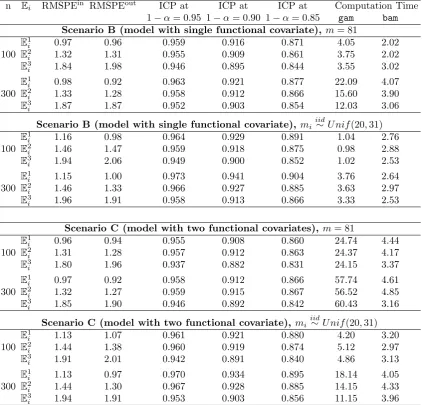
Table 1 summarizes the predictive performance of our method for these two scenarios.

We first discuss the case when the true function is non-linear (the top two panels in

Table 1). In this case, we observe that RMSPEin and RMSPEout from fitting the GFCM

are smaller than those from the linear FCM in all cases, indicating that the proposed

GFCM outperforms the linear FCM. The ICPs from the GFCM and the linear FCM are

fairly close to the nominal levels of 0.95, 0.90, and 0.85. However, on an average the

linear FCM produces larger intervals, indicated by larger IL values and wider range of

the estimated standard error denoted by R(SE) compared to the GFCM. Such patterns

confirm that the variability in prediction is not properly captured by the linear FCM when

the true model is non-linear. For less complicated error patterns such asE1

i (independent

error structure), both models produce smaller prediction errors; nevertheless GFCM still

produces smaller errors compared to linear FCM. The results are valid for different sample

sizes as well as for dense/sparse sampling designs. The bottom two panels of Table 1 show

the results when the underlying model is linear. In this case, the GFCM continues to show

very good prediction performance; the results are almost identical to the ones yielded by

the linear FCM irrespective of the number of subjects, sparseness of the sampling, and

the error covariance structure.

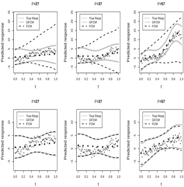
To aid understanding these results, Figure 1 displays prediction bands for three

subject-level trajectories, when the true model is non-linear (top panel) and linear

(bot-tom panel), and the covariates are observed densely. In the top panel, the prediction

bands for the linear FCM (dashed line) are much wider than the bands from the GFCM

(solid line). This indicates that variance estimation from the linear FCM is less accurate.

In the bottom panel, the prediction bands of the GFCM (grey solid line) and the linear

FCM (dashed line) are almost identical, indicating a similar performance in terms of the

variance estimation when the true model is linear.

Result from Scenario C: Now consider the setting involving two functional

covari-ates. In this experiment, we investigate both in-sample and out-of-sample prediction

performance as well as computational complexity of our algorithm with respect to the

number of additional covariates. It is worth noting that the computational complexity

can be affected by the number and the type of additional predictors as well as their

readily available irrespective of the number of terms in the model. Selecting the optimal

values of the smoothing parameters may be computationally demanding, and thus the

computational time depends on the number of smoothing parameters. There are two

available implementation tools to obtain predictions: gam and bam functions of mgcv

(Wood 2015) R package. Both functions provide almost identical model fits, but

com-putational advantage can be gained when using the bam function with very large data

sets. For completeness, we report simulation results for Scenario B (the model involving

a single functional covariate) and C.

We obtained the GFCM fits using 7 cubic B-splines for x1, x2 and t to model the

smooth functions F1(x1, t) and F2(x2, t). For estimation of the residual covariance, we

preset PVE = 99%. Table 2 summarizes RMSPEin, RMSPEout, ICP’s at the nominal

levels of 0.95, 0.90, and 0.85, and average computation time (in seconds). The

compu-tation time is measured on a 2.3GHz AMD Opteron Processor and averaged over 1000

Monte Carlo replications. The top and bottom post display the results corresponding

to Scenario B and C, respectively. We observe from the results that both in-sample

and out-of-sample predictive accuracy are still maintained irrespective of the number

of predictive variables. We also observe that the coverage (indicated by ICP) is fairly

close to the nominal levels in all cases. In terms of computational cost, both gam and

bam slightly increase the average computation time with the increased sample size and

model complexity. Nevertheless, the additional computation expense is rather minimal

compared to the computational time corresponding to single functional covariate. The

results also show that computations can be further sped up if bamis used.

To summarize, the numerical investigation shows that GFCM may result in significant

gain in prediction accuracy over the standard linear FCM, when the true model is

non-linear; GFCM has similar prediction performance relative to the linear FCM, when the

true model is linear. Furthermore, in the presence of two functional covariates, our

method still preserves high predictive accuracy, and the additional computation cost is

not substantial compared to the case of single functional covariate. Finally, although

results are not shown, we found that the above prediction performance is not sensitive

to the number of basis functions selected.

D.1 reports simulation results corresponding to another level of sparseness. Appendix

D.2 compares the results corresponding to two competitive approaches for covariance

estimation: using local linear smoothing Yao et al. (2005a) which is implemented in

Matlab using the functions of the PACE package and using a fast covariance smoothing

method (Xiao et al. 2016) which is implemented usingfpca.facefunction of therefund

R package (Huang et al. 2015).

5.2.2 Testing Performance

Now we assess the performance of the proposed testing procedure for the following two

scenarios: (A) E[Yd(t)|X1(t) = x1] = 1 + 2t+t2 +d(x1t/8); and (B) E[Yd(t)|X1(t) =

x1, X2(t) = x2] = 2t +t2 +x1sin(πt)/4 +d{2 cos(x2t)}. We generate the data

corre-sponding to the above true models using the error covariance structure and sampling

design defined in Section 5.1. In Scenario (A), whend= 0, the true model is a univariate

function of time point t, while when d > 0, the true model depends on both x1 and t.

Thus the parameter d indexes the departure from the null hypothesis given in (5). In

Scenario (B), the parameterd≥0 controls the departure from the null hypothesis given

in (7). For each of the scenarios, type I error of the test is investigated by settingd= 0,

and the power of the test is studied for positive values ofd. We generated 2000 samples

to assess the type I error rate, and 1000 samples to assess the power. The distribution

of the test statistic in (6) is approximated using B = 200 bootstrap samples for each

simulation.

Result from Scenario A: We first examine the size and power performance of the

global test presented in Algorithm 1. The empirical type I error rates are evaluated at

nominal levels of α = 5% and 10% for sample sizes 100 and 300, and the estimated

rejection probabilities are presented in top panel of Table 3. We observe that estimated

type I error rates are mostly within 2 standard errors of the nominal values, and the larger

sample size (n= 300) improves the size performance. The results also indicate that the

performance is similar across different covariance structures and sampling designs. The

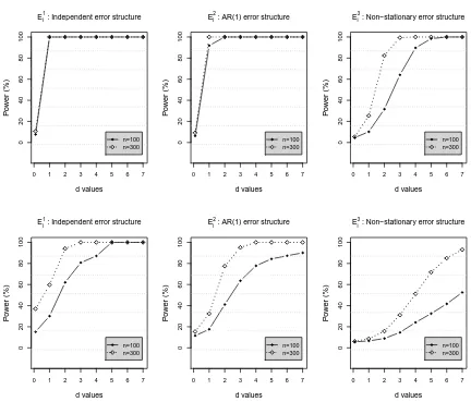
power performance of our proposed test is evaluated for a fixed nominal level α = 5%.

The top panel in Figure 2 displays the rejection probabilities for d = 0.1 ∼ 7 and for

sparse design. As expected, the power of the testing procedure increases with the sample

size, while the results are affected by the complexity of the error covariance: the power

corresponding to non-stationary error covariance is much lower than the counterpart

corresponding to AR(1) covariance error structure. Power curves for densely sampled

scenario are provided in the Supplementary materials, Appendix D.3. We found that the

results for densely sampled data are very similar to the one obtained for sparsely sampled

data.

Result from Scenario B: We now assess the size and power properties of the

signifi-cance testing presented in Algorithm 2. The bottom panel of Table 3 shows the empirical

type I error rates corresponding to nominal levels α= 5% and 10% for sample sizes 100

and 300. The results show that the estimated sizes are mostly within 2 standard errors of

the nominal values for all significance levels, and the results are less affected by different

error covariance structure and sampling designs. The bottom panel in Figure 2 displays

the rejection probabilities at the α = 0.05 level for d = 0.1 ∼ 7 and for different error

covariance structure; again, we only present the case corresponding to sparse design. For

the moderate sample size (n = 100), the power of the testing procedure increases with

the value ofd. For the larger sample size (n = 300) the empirical rejection probabilities

converge to 1 at a fast rate as the value of d increases. As expected, there is some loss

of power for complicated error pattern such asE3

i (non-stationary error covariance

struc-ture). However, the power performance for this case improves with the larger sample

size (n = 300). We also detected that the power of the test is affected by how the data

is sampled, but with only a negligible difference; the power curves corresponding to the

dense design are provided in the Supplementary materials, Appendix D.3.

Finally, it is worthwhile noting that, when calculating the size of proposed test Tn,obs

or T_b∗, the difference RSS0 −RSS1 occasionally comes out negative. We detected such

cases 2.6% of the time on an average, and this is true irrespective whether the sampling

design is dense or sparse. In these cases, we set RSS0−RSS1 = 0. Typically df0−df1

is positive. However, for very few cases (less than 0.1% of the time) this difference was

5.3

Applications

5.3.1 Gait Data

We turn our attention to data applications. We first consider the study of gait deficiency,

where the objective is to understand how the joints in hip and knee interact during a gait

cycle (Theologis 2009). Typically, one represents the timing of events occurring during a

gait cycle as a percentage of this cycle, where the initial contact of a foot is recorded as

0% and the second contact of the same foot as 100%. The data consist of longitudinal

measurements of hip and knee angles taken on 39 children as they walk through a single

gait cycle (Olshen et al. 1989; Ramsay and Silverman 2005). The hip and knee angles

are measured at 20 evaluation points {tj}20j=1 in [0,1], which are translated from percent

values of the cycle. Figure 1 of Appendix E.1 displays the observed individual trajectories

of the hip and knee angles.

We consider our proposed methodology to relate the hip and knee angles, and this is

an example of densely observed functional covariates and response. Let Yij = Yi(tj) be

the knee angle andWij =Xi(tj) +δij be the hip angle corresponding to theith child and

the percentage of gait cycle tj. Here δij are the measurement errors. We first employ

our resampling based test to investigate whether the hip angles are associated with the

knee angles. We select 7 cubic B-splines for x and t to fit the GFCM, E[Yi(t)|Xi(t)] =

F{Xi(t), t}, and B = 250 bootstrap replications are used. The bootstrap p-value is

computed to be less than 0.004, thus we conclude that the hip angle measured at a

specific time point has a strong effect on the knee angle at the same time point.

To assess how the hip and knee angles are related to each other, we fit our proposed

GFCM as well as the linear FCM. We assess the predictive accuracy by splitting the

data into training and test sets of size 30 and 9. Assuming that the hip angles are

observed with measurement errors, we smooth the covariate by FPCA and then apply

the center/scaling transformation. We compare prediction errors obtained by fitting both

the GFCM and the linear FCM. Also, as a benchmark model we further fit a linear mixed

effect (LME) modelYij = (β0+b0i) + (β1+b1i)Xij+ (β2+b2i)tij+ϵij, where (b0i, b1i, b2i)T

are the subject random coefficients from N(0, R) with some 3×3 unknown covariance

matrix R, ϵij are the errors from N(0, σϵ2), and (b0i, b1i, b2i)T and ϵij are assumed to be

out-of-sample RMSPE, the ICP, the IL and the R(SE). For the LME model, we report similar

measures, but we take average over the repeated measurements instead of integrating

over the time domain.

The results are summarized in Table 4 (top panel). We observe that the LME model

provides a poor predictive performance compared to the others, implying that models

in the framework of concurrent regression model are obviously better. GFCM yields

slightly better predictive performances relative to the linear FCM (negligible difference).

Specifically, the prediction errors from the GFCM are smaller than the linear FCM. The

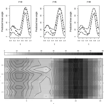
R(SE) obtained from the GFCM are narrower at all significance levels. Figure 3, top

panel, shows the prediction bands obtained for few subjects in the test data set. The two

competitive models, GFCM (solid line) and the linear FCM (dashed line), show similar

results. The bottom panel in Figure 3 displays a heat map plot of the predicted surface

using the GFCM. The results corroborate that the relationship between the hip angles and

the knee angles is linear. This finding is also confirmed by additional simulations results

using a generating model that mimics the gait data, which are included in Appendix E.2

of the Supplementary Materials.

5.3.2 Dietary Calcium Absorption Data

Next, we consider an application to dietary calcium absorption study (Davis 2002). In a

group of 188 patients, dietary and bone measurement tests are conducted approximately

every five years, and calcium intake and absorption are measured for each subject. The

patients are between 35 and 45 years old at the beginning of the study, with the overall

ages ranging from 35 to 64 years old. The number of repeated measurements per subject

varies between 1 to 4 times. This is an example of data where both the functional

response and covariate are observed on a sparse design. Our objective is to examine

the pattern of calcium absorption over the ages based on calcium intake as well as body

mass index (BMI) of the patients averaged over their ages. To assess their relationship,

let Yij = Yi(tij) be the calcium absorption and W1ij = X1,i(t1ij) +δij be the calcium

intake corresponding toith subject and the jth time point, where δij are the noise. Let

X2,i denote the average BMI for the ith subject. Figure 2 of Appendix E.1 displays the

at the visit.

In the analysis, we fit the GFCM, E[Yi(t)|X1,i(t), X2,i] = F{X1,i(t), t} +γ(t)X2,i,

where γ(t) denotes the unknown slope function of the average BMI. As an alternative

model, we also study the dependence assuming a linear FCM, E[Yi(t)|X1,i(t), X2,i] =

β0(t) +β1(t)X1,i(t) +γ(t)X2,i. In the analysis, ages are transformed into the values in

[0,1], and the results are considered as evaluation points of the functions. As before, we

begin by testing the null hypothesis of no association between the calcium intake and the

absorbtion. Specifically, we test the null hypothesis H0 : E[Y(t)|X1(t) =x1, X2 =x2] =

β0(t) +x2γ(t) versus the alternativeH1 : E[Y(t)|X1(t) =x1, X2 =x2] =F(x1, t) +x2γ(t)

using Algorithm 2. We select 7 cubic B-splines in directions x and t respectively to fit

the GFCM, and useB = 250 bootstrap replications. The p-value of our test is obtained

to be less than 0.003, indicating a significant association between the current calcium

intake measured and the current absorption.

We next analyze the predictive performance of the GFCM by using a training set

of 148 random patients and a test set formed by the remaining 40 patients. Shown

are also the results obtained with the linear FCM. Several adjustments are required to

accommodate the sparse sampling design of the covariates,X1,i(t). The covariates in the

training set are smoothed using the standard FPCA toolkit for sparse functional data

Yao et al. (2005a). The resulted estimated model (using the training data) is later used

to reconstruct the trajectories in the test set. The prediction results using the GFCM and

the competitive linear FCM are presented in Table 4 (bottom panel). Both the GFCM

and the linear FCM show similar in-sample and out-of-sample performance, RMSPEin

and RMSPEout_{; this indicates that a simple linear association between the calcium intake}

and absorption is more appropriate.

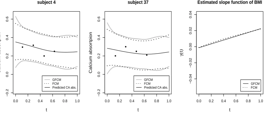
Furthermore, in Figure 4, the leftmost two panels present the point-wise prediction

intervals/bands for two selected subjects from the test data. The differences between the

GFCM (grey solid lines) and the linear FCM (dashed lines) are rather negligible, further

confirming a linearity dependence between the calcium intake and the absorption. The

rightmost panel in Figure 4 displays the estimated slope functionbγ(t) obtained by fitting

the GFCM and the linear FCM. On an average, both methods indicate a positive effect

Additional analysis has shown that the difference is due to the estimation errors.

6

Discussion

We propose a wider class of function-on-function regression models, the general

func-tional concurrent model, and discuss significance testing of no association. In particular,

our proposed hypothesis testing can formally assess whether the effect of a functional

covariate is significant under the assumption that the relationship between the response

and the predictor is general; the linear dependence is a special case of the proposed

gen-eral model, as described by our proposed modeling. In contrast, the existing literature

assumes a linear dependence between the response and the covariate/s. Thus, similar

significance tests are only valid when the linearity dependence assumption between the

response and the covariate is true. For the two applications - the gait data and the

dietary calcium absorption data - our testing procedure found significant association

between the response and covariate under a more general dependence assumption.

Fur-thermore, using the proposed methods we found evidence that the relationship between

the response and covariate is indeed linear; in contrast, the linear FCM assumes a linear

dependence is valid. Thus, our proposed procedure allows one to approach the problem

from a more general point of view. We have implemented our proposed estimation and

testing methodology usingRsoftware, and details about the implementation are provided

in Appendix F of the Supplementary Materials.

References

Davis, C. S. (2002). Statistical methods for the analysis of repeated measurements. New

York, NY: Springer.

Eilers, P. H. C. and B. D. Marx (1996). Flexible smoothing with b-splines and penalties.

Statistical Science 11, 89–121.

Goldsmith, J., S. Greven, and C. Crainiceanu (2013). Corrected confidence bands for

functional data using principal components. Biometrics 69, 41–51.

Goldsmith, J., V. Zipunnikov, and J. Schrack (2015). Generalized multilevel

Guo, W. (2002). Functional mixed effects models. Biometrics 58, 121–128.

Huang, L., F. Scheipl, J. Goldsmith, J. Gellar, J. Harezlak, M. W. McLean, B. Swihart,

L. Xiao, C. Crainiceanu, and P. Reiss (2015). refund: Regression with Functional Data.

R package version 0.1-13.

Jiang, C.-R. and J.-L. Wang (2011). Functional single index models for longitudinal data.

The Annals of Statistics 39, 362–388.

Li, Y. and D. Ruppert (2008). On the asymptotics of penalized splines. Biometrika 95,

415–436.

Malfait, N. and J. O. Ramsay (2003). The historical functional linear model. The

Canadian Journal of statistics 31, 115–128.

Marx, B. D. and P. H. C. Eilers (2005). Multivariate penalized signal regression.

Tech-nometrics 47, 13–22.

McLean, M. W., G. Hooker, A. M. Staicu, F. Scheipl, and D. Ruppert (2014). Functional

generalized additive models. Journal of Computational and Graphical Statistics 23,

249–269.

Morris, J. S. and R. J. Carroll (2006). Wavelet-based functional mixed models. Journal

of the Royal Statistical Society: Series B 68, 179–199.

Olshen, R. A., E. N. Biden, M. P. Wyatt, and D. H. Sutherland (1989). Gait analysis

and the bootstrap. The Annals of Statistics 17, 1419–1440.

Ramsay, J. O., G. Hooker, and S. Graves (2009). Functional data analysis in R and

Matlab. New York, NY: Springer.

Ramsay, J. O. and B. W. Silverman (2005). Functional data analysis (2nd ed.). New

York ; Berlin : Springer.

Reiss, P. T., L. Huang, and M. Mennes (2010). Fast function-on-scalar regression with

penalized basis expansions. International Journal of Biostatistics 6(28).

Ruppert, D., M. P. Wand, and R. J. Carroll (2003). Semiparametric regression.

Cam-bridge, New York: Cambridge University Press.

Scheipl, F., A. M. Staicu, and S. Greven (2015). Functional additive mixed models.

Journal of Computational and Graphical Statistics 24, 477–501.

Sent¨urk, D. and D. V. Nguyen (2011). Varying coefficient models for sparse