RL-SKAT: An Exact and Efficient Score Test for Heritability and Set Tests

(1)

| INVESTIGATION

RL-SKAT: An Exact and Ef

ﬁ

cient Score Test for

Heritability and Set Tests

Regev Schweiger,*,1_{Omer Weissbrod,}†_{Elior Rahmani,* Martina Müller-Nurasyid,}‡,§,_{** Sonja Kunze,}††,‡‡ Christian Gieger,††,‡‡_{Melanie Waldenberger,**},††,‡‡_{Saharon Rosset,}§§_{and Eran Halperin***},†††,‡‡‡ *Blavatnik School of Computer Science, Tel Aviv University, 6997801 Israel,†Department of Epidemiology, Harvard T.H. Chan School of Public Health, Boston, Massachusetts 02115,‡Institute of Genetic Epidemiology,††Institute of Epidemiology II, and ‡‡_{Research Unit of Molecular Epidemiology, Helmholtz Zentrum München, German Research Center for Environmental Health,} 85764 Neuherberg, Germany,§Department of Medicine I, Ludwig-Maximilians-Universität, 80336 Munich, Germany, **German Centre for Cardiovascular Research, Partner Site Munich Heart Alliance, 80336 Munich, Germany,§§School of Mathematical Sciences, Department of Statistics, Tel Aviv University, 69978 Israel, and ***Department of Computer Science,†††Department of Anesthesiology and Perioperative Medicine, and‡‡‡Department of Human Genetics, University of California, Los Angeles, California 90095 ORCID IDs: 0000-0003-2450-8901 (R.S.); 0000-0002-9017-2070 (E.R.); 0000-0001-6986-9554 (C.G.); 0000-0003-0583-5093 (M.W.); 0000-0002-4458-9545 (S.R.); 0000-0002-2373-3691 (E.H.)

ABSTRACTTesting for the existence of variance components in linear mixed models is a fundamental task in many applicativefields. In statistical genetics, the score test has recently become instrumental in the task of testing an association between a set of genetic markers and a phenotype. With few markers, this amounts to set-based variance component tests, which attempt to increase power in association studies by aggregating weak individual effects. When the entire genome is considered, it allows testing for the heritability of a phenotype, defined as the proportion of phenotypic variance explained by genetics. In the popular score-based Sequence Kernel Association Test (SKAT) method, the assumed distribution of the score test statistic is uncalibrated in small samples, with a correction being computationally expensive. This may cause severe inflation or deflation ofP-values, even when the null hypothesis is true. Here, we characterize the conditions under which this discrepancy holds, and show it may occur also in large real datasets, such as a dataset from the Wellcome Trust Case Control Consortium 2 (n = 13,950) study, and, in particular, when the individuals in the sample are unrelated. In these cases, the SKAT approximation tends to be highly overconservative and therefore underpowered. To address this limitation, we suggest an efficient method to calculate exactP-values for the score test in the case of a single variance component and a continuous response vector, which can speed up the analysis by orders of magnitude. Our results enable fast and accurate application of the score test in heritability and in set-based association tests. Our method is available inhttp://github.com/cozygene/RL-SKAT.

KEYWORDSstatistical genetics; SKAT; heritability; set-tests

T

HE variance component model is a well-established sta-tistical framework used in many scientiﬁcﬁelds. Testing for an association between several explanatory variables and a univariate response produces a variety of useful applications. For example, in metagenomics, an association is tested be-tween a phenotype (e.g., body mass index, blood glucose

levels, blood lipid levels, etc.) and the relative abundance counts of the measured species (Zhaoet al.2015).

In statistical genetics, testing for an association between a set of genetic markers and a phenotype, such as a disease or a trait, is a fundamental task. Since studies to detect genetic signals are often underpowered, even with large datasets becoming available, the common approach to help alleviate this issue is grouping together genetic markers and testing them jointly. Grouping genetic markers is commonly imple-mented under the framework of variance component models. In addition to association testing, this framework can be used to answer several questions, such as estimation of the underlying heritability of a phenotype (Kang et al. 2010); estimating the uncertainty of such estimation (Furlotteet al.

Manuscript received July 7, 2017; accepted for publication September 24, 2017; published Early Online October 12, 2017.

Supplemental material is available online atwww.genetics.org/lookup/suppl/doi:10. 1534/genetics.117.300395/-/DC1.

1_{Corresponding author: Blavatnik School of Computer Science, Schreiber Building,}

(2)

2014; Schweiger et al. 2016, 2017); phenotype prediction (Hayeset al.2001), and more.

We consider two main scenarios in which such tests are performed: (i) a single phenotype, many sets of markers and (ii) many phenotypes, a single set of markers. Scenario (i) is common in set-testing, where relatively few markers are tested jointly. This is particularly useful in the case of rare variants, which are increasingly available for study using sequencing technologies, and which constitute a large part of human genetic variability. In such studies, a single pheno-type is often tested against several sets of markers (for exam-ple, all rare variants in a single gene), because single-marker tests are often underpowered. Scenario (ii) occurs when studying heritability, defined as the proportion of phenotypic variance explained by genetics. Here, the tested markers are commonly the entire set of genotyped or sequenced single-nucleotide polymorphism (SNP) variants, or large portions of the genome (defined by,e.g., chromosome or functional annotation), and they are often tested against many (e.g., thousands) of phenotypes. Such phenotypes could be expres-sion profiles of genes (Priceet al.2011; Wrightet al.2014; Lloyd-Joneset al.2017), methylation levels across of various methylation sites in the DNA (Quonet al.2013; Van Dongen

et al.2016) or neuroimaging measurements (Ganjgahiet al.

2015; Geet al.2015).

Within the variance components framework, a common approach for association testing is the score test. It is used, for example, for testing the heritability of morphometric mea-surements derived from brain structural MRI scans (Geet al.

2015) and on fractional anisotropy measures in subjects from the Genetics of Brain Structure study (Ganjgahiet al.2015). The main popular alternative to the score test is the generalized likelihood ratio (LR) test,e.g., as implemented by GCTA, a popular software package for heritability estima-tion (Yanget al.2011). Both the score test and the LR test are based on properties of the likelihood function. The LR test statistic is calculated from the likelihood of the bestﬁtting model across different heritability values, and from the likeli-hood of the model corresponding to no heritability. Con-versely, the score test is based on the derivative of the likelihood function at the point corresponding to zero asso-ciation, and testing if it is signiﬁcantly nonzero. Compared with the LR test, the score test is often advantageous as it requires parameter estimation only for the null model, whereas the LR test requires parameter estimation for both the null and the alternative model. Additionally, the score test is the locally most powerful test; see Lippertet al.(2014) for a thorough comparison between the two tests, mainly in the context of set testing.

The Sequence Kernel Association Test (SKAT) (Wuet al.

2011) has become the standard score-based test in statistical genetics and in metagenomics (Zhao et al.2015), in large part due to its computational tractability. One of its merits is that it does not rely on the asymptotic distribution of the score test statistic, instead specifying a nonasymptotic distri-bution for the statistic under the null hypothesis of no

asso-ciation. However, it has been observed that this distribution may be inaccurate. In the SKAT-O extension (Leeet al.2012), a resampling-based moment-matching correction is suggested. An adaptive permutation testing procedure is suggested in Hasegawaet al.(2016). Chenet al.(2016) provide a method for calculating exactP-values; however, their method may be signiﬁcantly slower than that of SKAT, as it requires the eigendecomposition of a full rank square matrix, whose com-putational complexity is typically cubic in the sample size, for each distinct response variable (e.g., phenotype), or each set of explanatory variables (e.g., SNP set). Finally, in these works, it is reported that this discrepancy occurs mainly in studies having a small sample size, and it is currently unclear to which extent theP-values of SKAT are calibrated for large sample sizes.

Here, we undertake a thorough analysis of the null distri-bution of the score test statistic, and its discrepancy under the SKAT approximation. We suggest a practical way to quantify this discrepancy, and show that such discrepancies may occur even at large sample sizes. We show that a discrepancy is expected when the number of markers is comparable to or larger than the number of individuals, and when the individ-uals are relatively unrelated. In particular, in addition to such inaccuracies occurring in tests of sets of rare-variants in small samples, we conclude that they may also occur in large scale heritability studies. We further suggest a computational method, Recalibrated Lightweight SKAT (RL-SKAT), that allows exact P-value computation while maintaining computation time as in SKAT; in particular, for multiple phenotypes tested against the same marker set, only a single eigendecomposition is required. Finally, we demonstrate and validate our results on two real datasets, a large dataset from the Wellcome Trust Case Control Consortium 2 (International Multiple Sclerosis Genetics Consortiumet al.2011) (WTCCC2) study and the Cooperative health research in the Region of Augsburg (KORA) study (Holle

et al.2005) dataset.

Materials and Methods

We begin by reviewing the score test, as deﬁned by the SKAT method (Wuet al.2011) [see also the Supplementary Infor-mation in Lippertet al.(2014) for an excellent review]. We focus here on continuous phenotypes, and on the case of a single variance component; for other cases, see theDiscussion

below.

The variance components model

We consider the following standard variance components model [see Searleet al.(2009) for a detailed review]. Letn

(3)

encodes similarity between individuals. Then,yis assumed to follow:

y NXb;s2

gKþs2eIn

; (1)

The ﬁxed effects b and the coefﬁcients s2

g and s2e are the

parameters of the model.

In the context of statistical genetics,yis a vector of phe-notype measurements for each individual, andXis a matrix of covariates (often including an intercept, sex, age,etc.). LetZ be an3mstandardized (i.e., columns have zero mean and unit variance) genotype matrix containing the mSNPs we test. The common choice forKis a weighted dot product of the genetic markers (Yang et al. 2010); formally, deﬁne

K¼ZWZ⊤_;_where_W_{is a non-negative}_m₃_m_diagonal

ma-trix assigning a weight per SNP. A standard choice is the uniformWi;i¼1=m[see Wuet al.(2011) for a discussion].

The narrow-sense heritability due to genotyped common SNPs is deﬁned as the proportion of total variance explained by genetic factors (Visscheret al.2008):

h2 ¼ s

2 g

s2 gþs2e

: (2)

The score test

Under the above model, evaluating whether the tested cova-riates inﬂuence the response, while adjusting for additional covariates, corresponds to testing the null hypothesiss2

g¼0:

SKAT tests this hypothesis with a variance component score test in the corresponding mixed model. Speciﬁcally, the score statistic in the single-kernel case is obtained from the deriv-ative of the restricted likelihood, discarding terms that are constant with respect toy(Lippertet al.2014):

QðyÞ ¼y⊤SKSy (3)

where S¼In2XðX⊤XÞ21X⊤ is the projection matrix to the

subspace orthogonal to the covariatesX:For clarity of pre-sentation, we will divide the statistic bys2

e:Then,

Proposition 1:Letffigbe the eigenvalues ofSKS⊤and bex2

1;i are i.i.d. random variables distributed chi-square with one de-gree of freedom. Then,

Qs2_e X

n

i¼1

fix21;i: (4)

The proof of Proposition 1, as well as all proofs below, are deferred to the Supplemental Material inFile S1.

The exact distribution of the score test statistic

The above derivation is exact whenevers2e is known.

How-ever, in practice,s2

e is not known and needs to be estimated

from the data; most often, from the single response vector we are testing. In practice,s2

e is replaced with its restricted

max-imum likelihood (REML) estimate. The REML estimate is

simply the corrected mean of the squared entries of the phe-notype, after regressing out the covariates and usingS⊤S¼S:

^ s2

eðyÞ ¼ jjSyjj2

n2p ¼

y⊤_Sy

n2p: (5)

We note that sometimes the ML estimatey⊤Sy=nis used, or just y⊤Sy;as this only introduces a multiplicative constant, we use the unbiased REML estimate for simplicity of presenta-tion later. The statisticQands^2e;are, in fact, dependent random

variables. Therefore, the assumed distribution of Q=^s2e

(de-scribed in Proposition 1) does not hold when substitutings2 e

with its estimate,s^2e:In Zhang and Lin (2003), Liuet al.(2007,

2008), and Wuet al.(2011), this substitution is justiﬁed by the

claim that the (restricted) ML estimators^2e is consistent, and

may therefore be substituted by its true value for a large enough sample size,n. However, this argument does not take into consideration the dependency betweenQands^2

e:Also, as

shown below, this distribution might not hold in realistic set-tings. In Chen et al. (2016), this discrepancy is reported for small samples, and an exact distribution is derived for the sta-tisticQ=^s2e;and for anyn;KandX;which we review here:

Proposition 2:The distribution of Qs^2e may be modeled as a

ratio of quadratic forms of normal variables. In particular, if

zN ð0n;InÞ;then

Q ^ s2

e

¼dðn2pÞ z

⊤_SKSz

z⊤_Sz (6)

Assessing the discrepancy

While noted in the literature (Zhaoet al. 2015; Chenet al.

2016), the above discrepancy is reported for small samples only. However, as we show now, it may occur also when the number of individuals is large. We give a qualitative measure for when to expect large discrepancies between the asymp-totic approximation of a weighted mixture of chi-squares and the exact distribution.

In the Supplemental Material inFile S1, it is shown that the distributions ofQs2

eandQ

^ s2

e have the same means, but that

VarQs2 e

.VarQs^2e

;i.e., the latter has a smaller variance. We can further quantify the ratio between the variances as an indicator to the discrepancy between the distributions.

Proposition 3: Denote the eigenvalues ofSKSbyf1;. . .;fn;

and note that there are at most n2p nonzero eigenvaluesfi:

Denote the ﬁrst two sample moments of the eigenvalues by

f¼Pn

i¼1fi=ðn2pÞ and f2¼

Pn

i¼1f2i=ðn2pÞ: Denote the empirical variance of the eigenvalues bys2_ð_f_{Þ ¼}_f2₂_ð_f_Þ2

:Then,

R:5Var

Qs2e

VarQs^2_e¼

n2pþ2

n2p

sðfÞ f

₂2

þ1 !

(7)

(4)

dispersion. Therefore, the ratio becomes larger when the CV is smaller. Also, as noted above, since the approximation wrongly ignores the dependency between the statisticQand

^ s2

e;we expect the discrepancy to grow larger as the correlation

betweenQands^2e increases. We therefore examine this

corre-lation as an additional measure of this discrepancy.

Proposition 4: Let sðfÞ=f be the CV of the eigenvalues as

above. Then,

CorrQ;s^2_e¼ sðfÞ f

2

þ1 !₂1=2

(8)

This again demonstrates that CV affects discrepancy—the correlation becomes stronger when the CV is smaller. When

CV1; for example, when KIn; we have R1 and

R ðn2pþ2Þ=ðn2pÞ ð1þn=mÞ=ðn=mÞConversely, when

CV1;we haveR1 and CorrðQ;^s2eÞ 1=CV:This also

gives the variance ratio as the function of the correlation as

R¼n2pþ2

n2p

1

12Corr2Q;s^2_e: (9)

To summarize, the discrepancy is strong when the eigenvalues are more uniformly dispersed, and is weak when they have large variability. The dispersion of the eigenvalues of a kinship matrix has been previously shown to be related to the un-certainty in estimation of heritability: In Visscher and Goddard (2015), it is shown that the asymptotic variance of the herita-bility REML estimator decreases with the variance of the en-tries of the kinship matrix, and with the variance of the eigenvalues. In Schweigeret al.(2016), this result is shown without assumptions of asymptotics.

Examples:We now employ Propositions 3 and 4 to analyze

several interesting examples in a genetic context. For simplic-ity, in the following, we useX¼0;so thatp¼0 andS¼In:

Completely unrelated cohort: Suppose the cohort contains

completely unrelated individuals; then, K¼In: Thus,

f1¼. . .¼fn ¼1;soR ¼N;CorrðQ;s^2eÞ ¼1;andQ=^s 2 e is

the constantn. Compare this to the case wheres2

e is known;

then, it can be easily seen that Q=s2

e x2n: Therefore, the

mean is the same but the variance vanishes completely.

Rank-one kinship matrix: Consider the case of a simple

burden test (Leeet al.2012): if we assume the random effects sof all SNPs are identical, the burden test becomes

equiva-lent to the score test withK¼uu⊤;whereu¼Z1m: Alterna-tively, consider the extreme case, where all the individuals are identical:K¼11⊤ (while unlikely in human, this could be approximately true in studies of plants, yeast, etc.). In both these cases, there is a single nonzero eigenvalue:

f2¼. . .¼fn¼0; which gives R1 and CorrðQ;s^2eÞ ¼ ðf1=nÞ=

ffiffiffiffiffiffiffiffiffiffiffi f2₁₌

n

q

¼1 ffiffiffipn;that is, with large enough sample size, we expect the correlation to be effectively zero, and the SKAT mixture approximation to hold well.

A full rank kinship matrix: Assume the matrixZcontains

m.nSNPs in linkage equilibrium, where each column was mean-centered and normalized to have unit variance. Choos-ing the linear kernelK¼ZZ⊤=m;we follow Patterson et al.

(2006) in modelingZas a matrix of random standard normal variables, from which it follows thatKis a Wishart matrix. The limit distribution of the density of the eigenvalues ofKis spec-iﬁed by the Marčhenko-Pastur distribution (Marcenko and Pastur 1967), with itsﬁrst two moments known to be 1 and 1þn=m: Under this approximation, f1; f21þn=m; s2_ð_f_Þ_n₌_m_; _R_ð_n₂_p_þ₂_Þ₌_ð_n₂_p_{Þ ð}₁_þ_n₌_m_Þ₌_ð_n₌_m_Þ

and CorrQ;s^2e

1=pffiffiffiffiffiffiffiffiffiffiffiffiffiffiffiffiffiffi1þn=m: Whenmn; as is often the case, R1 and CorrðQ;s^2eÞ 1:This shows that, for a Table 1 Performance summary

Scenario Algorithm Exact? Preprocessing CalculatingQ=s^2

e CalculatingP-value

Heritability SKAT Approximate Oðnp2_þ_n2_p_þ_n3_Þ _O_ð_n2_Þ _O_ð_n_Þ

MiRKAT Exact Oðnp2_þ_n2_p_Þ _O_ð_n2_Þ _O_ð_n3_Þ

RL-SKAT Exact Oðnp2_þ_n2_p_þ_n3_Þ _O_ð_n2_Þ _O_ð_n_Þ

Set-testing SKAT Approximate Oðnp2_þ_nmp_þ_nm2_Þ _O_ð_n_ð_m_þ_p_ÞÞ _O_ð_n_Þ

MiRKAT Exact Oðnp2_þ_nmp_Þ _O_ð_n_ð_m_þ_p_ÞÞ _O_ð_n3_Þ

RL-SKAT Exact Oðnp2_þ_nmp_þ_n_ð_m_þ_p_Þ2_Þ _O_ð_n_ð_m_þ_p_ÞÞ _O_ð_n_Þ

Comparison of the different approaches forP-value calculation discussed. RL-SKAT achieves accuracy while remaining computationally efﬁcient.

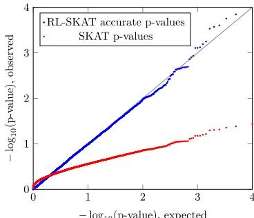
Figure 1 Statistic distribution. Results of the WTCCC2 data analysis, presented by quantile-quantile plots of the2log10ðpÞ-values for

(5)

large class of kinship matrices, we would expect the SKAT mixture approximation to hold poorly.

SNP set:Now, consider the case of set-testing, whereZis a normalized matrix of m,n SNPs in linkage equilibrium. Following the modeling above, we have againR ðn2pþ2Þ=

ðn2pÞ ð1þn=mÞ=ðn=mÞ and CorrQ;s^2e

1 ffiffiffiffiffiffiffiffiffipn=m;

whenmn;R1 and CorrQ;s^2e

pffiffiffiffiffiffiffiffiffim=n1;and thus expecting a good approximation by the mixture. This perhaps shows why the SKAT mixture approximation was considered good in the context of set-tests, when few variants or a large sample is considered. This also shows why, in small samples, the mixture is expected to be a poor approximation.

Calculating P-values

We now describe how to efﬁciently calculateP-values for the distribution of the statisticr¼Qy=^s2e

y calculated from the data; that is, given an observed statistic r, what is PrQs^2e.r

under the null? We review the result in Chen

et al.(2016):

Proposition 5:Let r be the observed value of the statistic.

De-note by að1rÞ;. . .;a ðrÞ

n the eigenvalues of SKS2r=ðn2pÞ S: Then,

Pr

Q ^ s2

e

.r

¼Pr X

n

i¼1

aðrÞ

i x

2 1;i.0

!

(10)

where x2

1;i are i.i.d. random variables distributed chi-square with one degree of freedom.

However, this condition requires us to calculate the eigen-values of SKS2r=ðn2pÞ S for each new value r, which, naively, has a complexity ofOðn3_Þ_:_{We consider two scenarios}

where this is problematic. First, in many heritability studies, we wish to test the heritability of many (e.g., thousands) of phe-notypes, all relative to the same kernel or kinship matrix (see above). For each phenotypey1;. . .;yN;we calculate its score test statisticri:ForP-value calculation, we need to compute the eigendecomposition ofSKS2ri=ðn2pÞ Sfor each observed statisticri;which is a signiﬁcant computational burden.

A second problematic scenario is of an association study of a single phenotype with many sets of SNPs,e.g., rare variants. Choosing a weighted linear kernel as in SKAT (Wu et al.

2011), we haveKi¼ZiWiZ⊤i for each set. AsKichanges with

each test, in principle, we need to perform a costly On3

eigendecomposition for each matrixKi:However, a signiﬁ-cant computational saving is gained due to the fact that the nonzero eigenvalues of SKiS¼SZiWiZ⊤iS are the same as

those ofW1_i=2Z⊤iSZiW 1=2

i ;which is anm3mmatrix (Lippert

et al.2014). As the number of tested SNPsmis often small,

calculating the eigenvalues of this matrix instead is signiﬁ-cantly faster, taking only Oðm3_Þ_; _{with matrix construction}

taking onlyOðnðmþpÞ2Þ(see Lippertet al.2014). However, with the exact approach, we need to calculate the eigen-values of SKiS2ri=ðn2pÞ Sinstead of SKiS: Even when

Kiis low rank, the matrixSKiS2ri=ðn2pÞ Smay be close

to full rank, so another approach is needed.

The following characterizes the eigenvalues ofSKS2r= ðn2pÞ Sgiven the eigenvalues ofSKS:

Proposition 6:Let r be the observed score test statistic. Denote

byf1;. . .;fnthe eigenvalues ofSKS:Denote the column space of a matrixAbycolðAÞ;its null space bykerðAÞ:Then,

Pr

Q ^ s2

e

.r

¼

Pr X

k

i¼1

fi2

r

n2p

x2

i;12

X

kþq

i¼kþ1 r n2px

2 i;1.0

! (11)

Figure 2 Heritability study. Histograms of theP-values of the studied phenotypes in the KORA dataset, as calcu-lated by the accurate method (left) and the inaccurate method (right). Histograms are shown in log-scale, and are capped atp¼1028_{for clarity of presentation. SKAT}

tends to severely deﬂateP-values, which are small accord-ing to the accurate calculation, leadaccord-ing to a severe loss of power.

(6)

where k¼rankðSKSÞis the number of nonzero eigenvaluesfi,

q¼dimðkerðSKSÞ\colðSÞÞ;and x2

1;i are i.i.d. random vari-ables distributed chi-square with one degree of freedom, i¼1;. . .;kþq:

Proposition 6 shows that calculating theP-value amounts to evaluating the cumulative distribution function of a certain weighted mixture of chi-square distribution at 0. This can be done rapidly using the Davies method (Davies 1980), which is based on the numerical inversion of the characteristic func-tion and runs in OðnÞ complexity, or using other methods (Duchesne and De Micheaux 2010).

It remains to calculatekandq. Naively, this can be done in

Oðn3_Þ_;_{for example by calculating the singular value}

decom-position (SVD) of SKSand Sto getk and to obtain vector bases for kerðSKSÞand colðSÞ;and by calculating the SVD of a matrix whose columns are the two vector bases to obtainq. When the same kernel is used with many phenotypes, it is a single preprocessing step. However, when the number of SNPs used to construct the kernel and the number of covariates are small, these quantities can be calculated much faster:

Proposition 7: Suppose K¼ZWZ⊤; and let k¼rankðSKSÞ

and q¼dimðkerðSKSÞ\colðSÞÞ:Then, k and q can be calcu-lated in complexity OðnðmþpÞ2Þ.

Most commonly,k¼minðm;nÞ21:When the number of SNPsmand the number of covariatespare small, the com-putational saving is substantial.

Data availability

This study makes use of data generated by the Wellcome Trust Case Control Consortium. A full list of the investigators who contributed to the generation of the data is available from

www.wtccc.org.uk. The data used in this manuscript were obtained via KORA.PASST (https://epi.helmholtz-muenchen. de/) with the following variables: KORA F4 Illumina Human-Methylation450K BeadChip array, BMIQ normalization KORA

F4 Affymetrix 6.0 SNP Array; imputed (HapMap2 reference panel). Access to the data may be obtained by request to KORA.

Results

Performance summary

We summarize the results described inMaterials and Methods

above in Table 1 and in Algorithms 1 and 2. We compare our method, RL-SKAT, with the SKAT formulation and the correc-tion of Chenet al.(2016) using the naive implementation of Proposition 5, as implemented by the MiRKAT software package (Zhao et al. 2015). The two scenarios discussed are those of a heritability study (sameKwith many responses yi) and SNP set-testing (many low rankKi). In all methods, a

preprocessing step of calculatingXyandffigis required. In a heritability study, calculating the statistic Q=^s2

e amounts to

evaluating two quadratic forms in Oðn2_Þ_: _{Compared to}

RL-SKAT, MiRKAT requires a fullOðn3_Þ_{eigendecomposition}

for each yi:For a set-testing study, these quadratic forms can be calculated inOðnðmþpÞÞdue to the low rank ofKi: Again, MiRKAT requires a fullOðn3_Þ _{eigendecomposition,}

compared to the OðnðmþpÞ2Þ procedure described in Proposition 7.

We now demonstrate our results on two datasets: a data-set from the Wellcome Trust Case Control Consortium 2 (International Multiple Sclerosis Genetics Consortium et al.

2011) (WTCCC2) study and the Cooperative health research in the Region of Augsburg (KORA) study (Holleet al.2005). A full description of data preprocessing is given in the Sup-plemental Material inFile S1.

A simulation study using WTCCC2 data

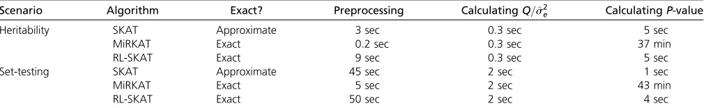
Weﬁrst analyze data with real genotypes from the WTCCC2 Multiple Sclerosis dataset, and simulated phenotypes. We used the same data processing described in Yang et al. Table 2 Benchmarks

Scenario Algorithm Exact? Preprocessing CalculatingQ=s^2

e CalculatingP-value

Heritability SKAT Approximate 3 sec 0.3 sec 5 sec

MiRKAT Exact 0.2 sec 0.3 sec 37 min

RL-SKAT Exact 9 sec 0.3 sec 5 sec

Set-testing SKAT Approximate 45 sec 2 sec 1 sec

MiRKAT Exact 5 sec 2 sec 43 min

RL-SKAT Exact 50 sec 2 sec 4 sec

Benchmark of the performance of different approaches forP-value calculation, applied to the KORA dataset.

Algorithm 1 RL-SKAT for heritability

procedurePREPROCESSINGðX;KÞ ⊳Preprocessing step, done once

CalculateXy5ðX⊤XÞ21

X⊤ ⊳Oðnp2_Þ

CalculateSKSusingS5I2XXy ⊳Oðn2_p_Þ

Calculateu1;. . .;un, the eigenvalues ofSKS ⊳Oðn3Þ

Extractk5rankðSKSÞ ⊳Oð1Þ

Calculateq5dimðkerðSKSÞ \_col_ð_S_ÞÞ_{using Proposition 7} _⊳_O_ð_n_ð_n1p_Þ2_Þ

procedureTESTðyÞ ⊳Calculate p-value for a single phenotypey

Calculate the score:r: 5Q=s^2_e5ðn2pÞ y⊤SKSy=y⊤Sy ⊳Oðn2_Þ

Calculatefað_irÞgas in Propositions 5 and 6 ⊳OðnÞ

Calculate the p-valuep5PrðPn_i₅1a ðrÞ

(7)

(2014), resulting inm = 360,556 SNPs forn = 13,950 in-dividuals. We constructed the kinship matrix by a standard, uniformly weighted linear kernel. We sought to demonstrate the discrepancy between the true null distribution and the chi-square weighted mixture distribution. Following Propo-sition 4, we calculated the correlation to be 0.886 and vari-ance ratio to beR¼4:69;indicating that a large discrepancy is possibly expected. To verify this, we simulated 10,000 ran-dom phenotypes, where each phenotype is a vector of i.i.d. standard normal variables. We tested whether the variance component is signiﬁcantly.0, and calculated theirP-values under the assumptions of either of the two distributions. In Figure 1, we show the quantile-quantile plots for the two sets ofP-values. As evidenced, using the SKAT mixture dis-tribution results in a severe deﬂation of small P-values, while using the correct distribution as in Proposition 1 re-sults in an accurate P-value distribution. This shows that even for large sample sizes (n = 13,950), such a discrep-ancy is possible.

Testing for heritable methylation sites in the KORA dataset

The longitudinal KORA study consists of whole-blood meth-ylation levels and genotypes of n = 1799 individuals. The phenotype is the proportion of methylated samples at a spe-ciﬁc site, averaged across DNA samples of an individual. The study consists of independent population-based subjects from the general population living in the region of Augsburg, southern Germany (Holleet al.2005). Whole-blood samples of the KORA F4 study were used as described elsewhere (Pfeiffermet al.2015). In summary, a total of 431,366 meth-ylation site phenotypes, and 657,103 SNPs, were available for analysis. The correlation as in Proposition 4 is 0.976 and the variance ratio isR¼22:01;indicating again that a large discrepancy is expected. We performed a heritability study of multiple phenotypes with the same kinship matrix, by testing the heritability of theN = 43,140 methylation sites on chro-mosome 1. As it is common for a methylation site to be cor-related with its surrounding SNPs (Gibbset al.2010; Zhang

et al.2010; Bellet al.2011), we avoided suchciseffects by

using a kinship matrix constructed from the m = 604,170 SNPs on all chromosomes other than 1. The kinship ma-trix is constructed by a standard, uniformly weighted linear kernel. For covariates, we used Xconsisting only

of an intercept vector. Again, we calculatedP-values under the assumption of the two distributions. We note that it has been shown that some methylation site profiles often display significant heritability, while others do not; thus, both significant and insignificant P-values are expected (Rahmaniet al.2017).

In Figure 2 we show the histograms of the log10of theP-value

of all the considered phenotypes. The two histograms are indeed very different; P-values calculated using the inaccurate SKAT mixture distribution indicate that the heritability of almost all sites is considered insigniﬁcant; for example, using a Bonferroni threshold of 0:051=431401026_; _{only 8/43,140 sites are}

significant. In light of the results above, it is reasonable to suspect that P-values of many heritable phenotypes are de-flated, thus causing false negatives. TheP-values distribution has a peak at0.5, likely an artifact of the inaccurate calcula-tion method. In comparison,P-values calculated by RL-SKAT do not exhibit such a peak. They are significantly smaller, and using the same Bonferroni threshold, we now find 319/43,140 significant sites. Indeed, a simulated power study of both approaches under varying degrees of a true underlying heritability validates that the inaccurate approach results in a severe decrease in power (Figure 3), which has been reported in the literature (Uemotoet al.2013). As a point of reference, we compared the power of RL-SKAT with that of the popular LR test approach, and found they have similar power (see the Supplemental Material inFile S1). We conclude that in this dataset, using the SKAT distribution forP-value calculation is highly problematic.

Benchmarks

Finally, we benchmarked the methods discussed here on the KORA dataset under the two above scenarios, on a 64G, 2.2 GHz Linux workstation, using our implementation in the Python language. We verified that the relevant part of our implementation is equivalent to MiRKAT and has a very similar running time. For the scenario of heritability testing, we calculated theP-values of 1000 phenotypes with the kin-ship matrix. For the scenario of set testing, we used 1000 sets of 100 SNPs each. The results are summarized in Table 2; as expected, the computational savings are very significant, achieving a speedup of more than two orders of magnitude. We expect the speedup to be even more significant for larger datasets.

Algorithm 2 RL-SKAT for set-tests

procedurePREPROCESSING(X;ZW1=2) ⊳Preprocessing step, done once

CalculateXy5ðX⊤XÞ21X⊤ ⊳Oðnp2_Þ

CalculateSZW1=2usingS5I2XXy ⊳OðnmpÞ

Calculateu1;. . .;unas the squares of the singular values ofSZW1=2 ⊳Oðnm2Þ

Extractk5rankðSKSÞ ⊳Oð1Þ

Calculateq5dimðkerðSKSÞ \_col_ð_S_ÞÞ_{using Proposition 7} _⊳_O_ð_n_ð_m1p_Þ2_Þ

procedureTEST(y) ⊳Calculate p-value for a single phenotypey

Calculate the score:r: 5Q=s^2

e5ðn2pÞ y⊤SKSy=y⊤Sy;usingK5ZWZ⊤ ⊳Oðnðm1pÞÞ

Calculatefað_irÞgas in Propositions 5 and 6 ⊳OðnÞ

Calculate the p-valuep5PrðPn_i₅1a ðrÞ

(8)

Discussion

In summary, we have shown that the distribution suggested by SKAT to the score test statistic may be very inaccurate. Unlike previous studies, which have noted this discrepancy only in small sample sizes, we have shown that it might occur in large studies as well. We have proposed a computational method to accurately calculateP-values without compromising compu-tational time. Finally, we demonstrated ourﬁndings in two datasets.

The exact calculation ofP-values can be applied to other variants of the score test; for example, the SKAT-O (Leeet al.

2012) test seeks to ﬁnd an optimal combination of burden tests and nonburden tests, which amounts to the score test with a certain kernel.

In this work, we focused on the case of a single kernel, and on a continuous phenotype. The extension of this work to multiple kernels (e.g., corresponding to several sets of SNPs) or to binary phenotypes (e.g., case/control studies) is non-trivial, as the null distribution cannot be modeled as a ratio of quadratic forms (see, e.g., Wang 2016; Wu et al.2016). It therefore remains a subject for future work.

We believe that the prominence of likelihood-ratio based tests in heritability studies might stem from the statistical issues discussed above (see, for example, Uemotoet al.2013), where SKAT was found to be signiﬁcantly less powerful. It is our hope that this paper would facilitate the use of score tests in heritability studies in the future.

Acknowledgments

R.S. is supported by the Colton Family Foundation. This study was supported in part by a fellowship from the Edmond J. Safra Center for Bioinformatics at Tel Aviv University to R.S. and E.R. E.H was partially supported by NSF grant 1705197. Funding for the project was provided by the Wellcome Trust under award 076113. The KORA study was initiated andﬁnanced by the Helmholtz Zentrum München, German Research Center for Environmental Health, which is funded by the German Federal Ministry of Education and Researchand by the State of Bavaria. Furthermore, KORA research was supported within the Munich Center of Health Sciences, Ludwig-Maximilians-Universität, as part of LMUinnovativ.

Literature Cited

Bell, J. T., A. A. Pai, J. K. Pickrell, D. J. Gaffney, R. Pique-Regiet al., 2011 DNA methylation patterns associate with genetic and gene expression variation in hapmap cell lines. Genome Biol. 12: R10.

Chen, J., W. Chen, N. Zhao, M. C. Wu, and D. J. Schaid, 2016 Small sample kernel association tests for human genetic and microbiome association studies. Genet. Epidemiol. 40: 5–19. Davies, R. B., 1980 Algorithm AS 155: the distribution of a linear combination of_x2_{random variables. J. R. Stat. Soc. Ser. C Appl.}

Stat. 29: 323_–333.

Duchesne, P., and P. L. De Micheaux, 2010 Computing the distri-bution of quadratic forms: further comparisons between the Liu-Tang-Zhang approximation and exact methods. Comput. Stat. Data Anal. 54: 858–862.

Furlotte, N. A., D. Heckerman, and C. Lippert, 2014 Quantifying the uncertainty in heritability. J. Hum. Genet. 59: 269–275. Ganjgahi, H., A. M. Winkler, D. C. Glahn, J. Blangero, P. Kochunov

et al., 2015 Fast and powerful heritability inference for family-based neuroimaging studies. Neuroimage 115: 256–268. Ge, T., T. E. Nichols, P. H. Lee, A. J. Holmes, J. L. Roffmanet al.,

2015 Massively expedited genome-wide heritability analysis (MEGHA). Proc. Natl. Acad. Sci. USA 112: 2479–2484. Gibbs, J. R., M. P. van der Brug, D. G. Hernandez, B. J. Traynor, M.

A. Nallset al., 2010 Abundant quantitative trait loci exist for DNA methylation and gene expression in human brain. PLoS Genet. 6: e1000952.

Hasegawa, T., K. Kojima, Y. Kawai, K. Misawa, T. Mimori et al., 2016 AP-SKAT: highly-ef_ﬁcient genome-wide rare variant as-sociation test. BMC Genomics 17: 745.

Hayes, B., M. Goddard, and M. E. Goddard, 2001 Prediction of total genetic value using genome-wide dense marker maps. Ge-netics 157: 1819–1829.

Holle, R., M. Happich, H. Löwel, and H. Wichmann MONICA/ KORA Study Group, 2005 KORA - a research platform for pop-ulation based health research. Gesundheitswesen 67: S19–S25. International Multiple Sclerosis Genetics Consortium Wellcome Trust Case Control Consortium 2Sawcer, S., G. Hellenthal, M. Pirinen, C. C. Spencer, N. A. Patsopouloset al., 2011 Genetic risk and a primary role for cell-mediated immune mechanisms in multiple sclerosis. Nature 476: 214–219.

Kang, H. M., J. H. Sul, S. K. Service, N. A. Zaitlen, S.-y. Konget al., 2010 Variance component model to account for sample struc-ture in genome-wide association studies. Nat. Genet. 42: 348– 354.

Lee, S., M. J. Emond, M. J. Bamshad, K. C. Barnes, M. J. Riederet al., 2012 Optimal uniﬁed approach for rare-variant association test-ing with application to small-sample case-control whole-exome sequencing studies. Am. J. Hum. Genet. 91: 224–237.

Lippert, C., J. Xiang, D. Horta, C. Widmer, C. Kadie et al., 2014 Greater power and computational ef_ﬁciency for kernel-based association testing of sets of genetic variants. Bioinfor-matics 30: 3206_–3214.

Liu, D., X. Lin, and D. Ghosh, 2007 Semiparametric regression of multidimensional genetic pathway data: least-squares kernel machines and linear mixed models. Biometrics 63: 1079_–1088. Liu, D., D. Ghosh, and X. Lin, 2008 Estimation and testing for the effect of a genetic pathway on a disease outcome using logistic kernel machine regression via logistic mixed models. BMC Bio-informatics 9: 292.

Lloyd-Jones, L. R., A. Holloway, A. McRae, J. Yang, K. Smallet al., 2017 The genetic architecture of gene expression in peripheral blood. Am. J. Hum. Genet. 100: 228–237.

Marcenko, V. A., and L. A. Pastur, 1967 Distribution of eigen-values for some sets of random matrices. Math. USSR-Sbornik 1: 457.

Patterson, N., A. L. Price, and D. Reich, 2006 Population structure and eigenanalysis. PLoS Genet. 2: e190.

Pfeifferm, L., S. Wahl, L. C. Pilling, E. Reischl, J. K. Sandlinget al., 2015 DNA methylation of lipid-related genes affects blood lipid levels. Circ. Cardiovasc. Genet. 8: 334–342.

Price, A. L., A. Helgason, G. Thorleifsson, S. A. McCarroll, A. Kong

et al., 2011 Single-tissue and cross-tissue heritability of gene expression via identity-by-descent in related or unrelated indi-viduals. PLoS Genet. 7: e1001317.

(9)

Rahmani, E., L. Shenhav, R. Schweiger, P. Youseﬁ, K. Huenet al., 2017 Genome-wide methylation data mirror ancestry informa-tion. Epigenetics Chromatin 10: 1.

Schweiger, R., S. Kaufman, R. Laaksonen, M. E. Kleber, W. März

et al., 2016 Fast and accurate construction of conﬁdence in-tervals for heritability. Am. J. Hum. Genet. 98: 1181–1192. Schweiger, R., E. Fisher, E. Rahmani, L. Shenhav, S. Rossetet al.,

2017 Using stochastic approximation techniques to efﬁciently construct conﬁdence intervals for heritability, pp. 241–256 in

International Conference on Research in Computational Molecular Biology. Springer, Berlin.

Searle, S. R., G. Casella, and C. E. McCulloch, 2009 Variance Components, Vol. 391. John Wiley & Sons, Hoboken, NJ. Uemoto, Y., R. Pong-Wong, P. Navarro, V. Vitart, C. Haywardet al.,

2013 The power of regional heritability analysis for rare and common variant detection: simulations and application to eye biometrical traits. Front. Genet. 4: 232.

Van Dongen, J., M. G. Nivard, G. Willemsen, J.-J. Hottenga, Q. Helmeret al., 2016 Genetic and environmental inﬂuences in-teract with age and sex in shaping the human methylome. Nat. Commun. 7: 11115.

Visscher, P. M., and M. E. Goddard, 2015 A general uniﬁed frame-work to assess the sampling variance of heritability estimates using pedigree or marker-based relationships. Genetics 199: 223–232. Visscher, P. M., W. G. Hill, and N. R. Wray, 2008 Heritability in the

genomics era—concepts and misconceptions. Nat. Rev. Genet. 9: 255–266.

Wang, K., 2016 Boosting the power of the sequence kernel asso-ciation test by properly estimating its null distribution. Am. J. Hum. Genet. 99: 104_–114.

Wright, F. A., P. F. Sullivan, A. I. Brooks, F. Zou, W. Sunet al., 2014 Heritability and genomics of gene expression in periph-eral blood. Nat. Genet. 46: 430–437.

Wu, B., W. Guan, and J. S. Pankow, 2016 On efﬁcient and ac-curate calculation of signiﬁcance p-values for sequence kernel association testing of variant set. Ann. Hum. Genet. 80: 123– 135.

Wu, M. C., S. Lee, T. Cai, Y. Li, M. Boehnke et al., 2011 Rare-variant association testing for sequencing data with the se-quence kernel association test. Am. J. Hum. Genet. 89: 82–93. Yang, J., B. Benyamin, B. P. McEvoy, S. Gordon, A. K. Henderset al., 2010 Common SNPs explain a large proportion of the herita-bility for human height. Nat. Genet. 42: 565–569.

Yang, J., S. H. Lee, M. E. Goddard, and P. M. Visscher, 2011 GCTA: a tool for genome-wide complex trait analysis. Am. J. Hum. Genet. 88: 76–82.

Yang, J., N. A. Zaitlen, M. E. Goddard, P. M. Visscher, and A. L. Price, 2014 Advantages and pitfalls in the application of mixed-model association methods. Nat. Genet. 46: 100–106. Zhang, D., and X. Lin, 2003 Hypothesis testing in semiparametric

additive mixed models. Biostatistics 4: 57–74.

Zhang, D., L. Cheng, J. A. Badner, C. Chen, Q. Chen et al., 2010 Genetic control of individual differences in gene-speciﬁc methylation in human brain. Am. J. Hum. Genet. 86: 411–419. Zhao, N., J. Chen, I. M. Carroll, T. Ringel-Kulka, M. P. Epsteinet al., 2015 Testing in microbiome-proﬁling studies with MiRKAT, the microbiome regression-based kernel association test. Am. J. Hum. Genet. 96: 797–807.