Implementation of Direct Displacement-Based Design for Highway Bridges

(1)

ABSTRACT

SUAREZ, VINICIO A. Implementation of Direct Displacement-Based Design for Highway Bridges. (Under the direction of Dr. Mervyn Kowalsky).

In the last decade, seismic design shifted towards Displacement-Based methods. Among the several methodologies that have been devolved, the Direct Displacement-Based Design Method (DDBD) has been shown to be effective for performance-based seismic design of bridges and other types of structures.

The main objective of this Dissertation is to bridge the gap between existing research on Direct Displacement-Based Design (DDBD) and its implementation for design of conventional highway bridges.

Real highway bridges have complexities that limit the application of DDBD. This research presents new models to account for: limits in the lateral displacement capacity of the superstructure, skewed configurations, P-Δ effects, expansion joints and different types of substructures and abutments. Special interest is given to the definition of predefined displacement patterns that can be used for direct application of DDBD to several types of bridges.

The results of the research show the effectiveness of the proposed models. One of the most relevant conclusions is that bridge frames of bridges with seat-type abutments, which comply with the balanced mass and stiffness requirements of AASHTO, can be designed with DDBD using rigid body translation patters, which greatly simplifies the application of DDBD.

Another objective of the research was to compare the execution and outcome of DDBD to the design method in the new AASHTO Guide Specifications for LRFD Seismic Bridge Design. This was accomplished by a comparative study of four real bridges designed with the two methods. Results of that study indicate that DDBD is compatible with the new AASHTO Guide Specification and furthermore, it has several advantages over the design method in that specification.

(2)

Implementation of Direct Displacement Based Design for Highway Bridges by

Vinicio A. Suarez

A dissertation submitted to the Graduate Faculty of North Carolina State University

in partial fulfillment of the requirements for the Degree of

Doctor of Philosophy Civil Engineering

Raleigh, North Carolina 2008

APPROVED BY:

______________________ _______________________

Dr. Vernon Matzen Dr. James Nau

______________________ ________________________

Dr. Mohammed Gabr Dr. Lewis Reynolds

(3)

ii

BIOGRAPHY

Vinicio Suarez was born in Cuenca, Ecuador on February 23th, 1975. He received his BS in Civil Engineering, in December 2000, from Universidad Tecnica Particular de Loja (UTPL), in Ecuador. After graduating, he jointed the School of Engineering at UTPL as faculty member and taught courses on Strength of Materials and Reinforced Concrete. In August of 2004, he came to Raleigh and joined North Carolina State University to obtain a Master of Science Degree in 2005. After that, he started Doctoral studies, which he completed in 2008, obtaining the Degree of Doctor of Philosophy in Civil Engineering. His research interests include but are not limited to the seismic analysis and design bridges and buildings, soil-structure interaction and software development. After completion of his PhD, Vinicio will return to Ecuador as a Professor, Director of the Civil Engineering School and Director of the Civil Engineering, Geology and Mining Research Center at UTPL.

(4)

iii

ACKNOWLEDGMENTS

I wish to thank my advisor, Dr. Mervyn Kowalsky, for his continuous support and generosity in passing on his knowledge to me. I also want to thank the other members of the Advisory Committee, Dr. Vernon Matzen, Dr. Mohammed Gabr, Dr. James Nau and Dr. Lewis Reynolds.

I would not have done this without the love of my wife, María del Rocío and the support of of UTPL and its Chancellor Dr. Luis Miguel Romero. I also thank my friends in NCSU especially Brent Robinson and Luis Mata for their continuous support.

Finally, I would like to thank the financial support provided by NCSU, UTPL and SENACYT.

(5)

iv

LIST OF TABLES

PART I

Table 1 - Models for equivalent linearization ……….. 9

PART II Table 1. Parameters for hysteretic damping models in drilled shaft - soil systems ………… 24

Table 2. Displacement patterns for DDDBD of bridges ……… 27

Table 3 - Parameters for DDBD of common types of piers ………... 34

Table 4 - Parameters to define Eq.15 for far fault sites ………... 40

Table 5 - Parameters to define Eq.15 for near fault sites ……….. 40

Table 6 - Design parameters from local to global axes ……….. 70

Table 7 - Design results for multi-column bent ………. 71

Table 8 - Design results for multi-column bent ………. 72

Table 9 - Target displacements Trial design CA-1………. 75

Table 10 - Transverse design parameters ……… 77

Table 11 - Longitudinal design parameters ……… 78

Table 12 – Element design parameters ……….. 79

PART III Table 1- Parameters for hysteretic damping models in drilled shaft - soil systems …………88

Table 2 - Displacement patterns for DDDBD of bridges ………... 91

Table 3 - Summary of bridges used for trial designs ………. 91

Table 4 - Moment curvature analysis results for bent in bridge MO-1………... 95

Table 5 - Design results for MO-1 ………... 106

Table 6 - Moment-Curvature analysis results for LRFD Seismic design of bent in Bridge MO-2 ……… 109

Table 7 - Design Results for MO-2 ……….. 114

Table 8 - LRFD-Seismic design summary for trial design IL-2 ……….. 118

(8)

vii

Table 10 - DDBD results for trial design IL-2 ………. 124

Table 11 - Comparison of design results for trial design IL-2 ………. 125

Table 12 - Target displacements Trial design CA-1 ……… 130

Table 13. Transverse Design. CA-1 ………. 133

Table 14. Longitudinal Design parameters. Trial design CA-1 ………... 134

Table 15. Bent design. Trial design CA-1 ……… 135

Table 16. Summary of LDFD-Seismic and DDBD designs ……… 136

PART IV Table 1 - Bridge Frames ……….. 161

Table 2 - Continuous Bridges with seat-type abutments ……… 162

Table 3 - Integral abutment bridge table ……….. 169

Table 4 - Displacement patterns for DDDBD of bridges ……… 173

PART V Table 1 - Parameters for hysteretic damping models in drilled shaft - soil systems ……… 181

Table 2 - Parameters to define Eq.15 for far fault sites ……….. 182

Table 3 - Parameters to define Eq.15 for near fault sites ……….... 182

Table 4 - Yield displacement and equivalent model parameters for bent in sand ………... 189

Table 5 - In-plane damage-based target displacements for drilled shaft bent in sand …… 190

Table 6 - In-plane stability-based target displacements for drilled shaft bent in sand …... 191

Table 7 - In-plane design results for drilled shaft bent in sand ……….. 193

Table 8 - Bridge parameter matrix ……….. 202

Table 9 - DDBD results for bridge group ……….... 203

PART VI Table 1- Classification of bridges and design algorithms ……… 212

Table 2 - Target displacements Trial design CA-1 ……….. 228

Table 3 - Transverse Design. CA-1 ………... 231

Table 4 - Longitudinal Design parameters. Trial design CA-1 ………... 231

Table 5 - Bent design. Trial design CA-1 ……… 232

(9)

viii

LIST OF FIGURES

PART I

Figure 1 - Effects of earthquake motion on inelastic SDOF ……… 5

Figure 2 - Linearization Methods ……… 7

Figure 3 - Acceleration Response spectrum ……….. 11

Figure 4 - Equivalent damping models translated to displacement coefficient ………. 12

Figure 5 - Displacement coefficient models translated to equivalent damping ………. 12

Figure 6 - C coefficient for elastoplastic systems in sites class B. (FEMA, 2006) ……….... 13

PART II Figure 1 - Equivalent linearization approach used in DDBD ……… 21

Figure 2 - Equivalent single degree of system ………... 22

Figure 3 - Determination of effective period in DDBD ……… 23

Figure 4 - Equivalent damping models for bridge piers ………... 25

Figure 5 - DDBD main steps flowchart ………... 26

Figure 6 - Complementary DDBD flowcharts ………... 26

Figure 7 - Curve bridge unwrapped to be designed as straight ……….. 31

Figure 8 - Assumed superstructure displacement pattern ……….. 33

Figure 9 - Common types of piers in highway bridges ……….. 36

Figure 10 - Le and a for definition of the equivalent model for drilled shaft bents (Suarez and Kowalsky, 2007) ……….... 37

Figure 11 - Ductility vs. C for far fault sites ………. 41

Figure 12 - Ductility vs. C for near fault sites ……… 41

Figure 13 - Design axes in skewed elements ……….... 42

Figure 14 - Displacement patterns for bridges with expansion joints ………... 45

Figure 15 - Longitudinal displacement pattern for bridges with expansion joints ………… 46

Figure 16 - Strength distribution in the longitudinal and transverse directions ………. 47

Figure 17 - 2D model of bridge with secant stiffness ……….... 52

(10)

ix Figure 19 - Force-displacement response of bents designed for combinations of seismic and

non-seismic forces ……….. 60

Figure 20 - Two span continuous bridges ……….. 66

Figure 21 - Target ductility of central pier of two span bridge ……….. 67

Figure 22 - Single Column Bent ………. 68

Figure 23 - Stability based ductility vs. aspect ratio for a single column pier ………... 69

Figure 24 - Multi column bent ……… 69

Figure 25 - Displacement spectrum and displacement spectra of 7 earthquake compatible records ……… 71

Figure 26 - Elevation view three span bridge ……… 72

Figure 27 - Superstructure section and interior bent ……….. 73

Figure 28 - Displacement Spectra ……….. 74

PART III Figure 1 - Equivalent linearization approach used in DDBD ……… 85

Figure 2 - Equivalent single degree of system ………... 85

Figure 3 - Determination of effective period in DDBD ……… 87

Figure 4 - Equivalent damping models for bridge piers ……… 88

Figure 5 - DDBD main steps flowchart ………. 89

Figure 6 - Complementary DDBD flowcharts ………... 90

Figure 7 - Design spectra ……… 92

Figure 8 - Elevation view MO-1 bridge ……… 93

Figure 9 - Central bent MO-1 bridge ………. 93

Figure 10 - Determination of disp. demand for LRFD Seismic design of bridge MO-1 ….. 96

Figure 11- Determination of effective period for DDBD of bridge MO-1 ……….. 102

Figure 12 - Moment curvature response of RC column of diameter 1.07 m with 1% steel 104 Figure 13 - α β γ factors of UCSD modified model ……… 105

Figure 14 - Elevation view MO-2 Bridge ……… 107

Figure 15 - Interior bent in MO-2 Bridge ……… 108

(11)

x

Figure 17 - Effective period for interior bent of bridge MO-2 ……… 113

Figure 18 - Moment curvature response of 0.9 diameter RC section with 2.6% steel ……. 113

Figure 19 - Elevation view of trial design IL-2 ……… 115

Figure 20 - Interior bent trial design IL-02 ……….. 116

Figure 21 - Cracked to gross inertia ratio for circular RC sections (Imbsen, 2007) ……… 117

Figure 22- 2D bridge model for static analysis ……… 122

Figure 23 - Elevation view trial design CA-1 ……….. 126

Figure 24 - Superstructure section and interior bent, trial design CA-1 ……….. 127

PART IV Figure 1 - Equivalent single degree of system ………. 158

Figure 2 - DDBD main steps flowchart ……… 158

Figure 3 - Complementary DDBD flowcharts ……… 159

Figure 4 - Displacement design spectrum and compatible records ………. 160

Figure 5 - Superstructure type and properties ………. 160

Figure 6 - Regularity indexes for bridge frames ………. 163

Figure 7 - Regularity indexes for bridges with seat-type abutments ……….. 164

Figure 8 - Performance indexes for bridge frames. ………. 165

Figure 9 - Performance indexes for Bridges with seat-type abutments ………... 166

Figure 10 - Design and analysis results for bridge 1.7……….. 167

Figure 11 - Design and analysis results for bridge 3.9 ………. 168

Figure 12 - Displacement pattern for a bridge with integral abutments ………... 168

Figure 13 - Design and ITHA results for bridges with integral abutments ……….. 170

Figure 14 - Displacement patterns for bridges with expansion joints ……….. 171

Figure 15 - Symmetric bridge with one expansion joint ……….. 171

Figure 16 - Asymmetric bridge with one expansion joint ……… 172

Figure 17 - Asymmetric bridge with two expansion joints ……….. 172

PART V Figure 1 - Equivalent linearization ………... 175

(12)

xi

Figure 3 - Complementary DDBD flowcharts ………. 177

Figure 4 - Determination of the effective period ……….. 178

Figure 5 - Equivalent damping models for bridge piers ……….. 182

Figure 6 - P-Δ Ductility for far fault sites ……… 183

Figure 7 - P-Δ Ductility for near fault sites ………. 184

Figure 8 - Drilled shaft bent is sand ………. 185

Figure 9 - Displacement design spectra form SDC D, C and B ……….. 186

Figure 10 - a) In-plane target displacement vs. aspect ratio. b) In-plane target ductility vs. aspect ratio ……… 191

Figure 11 - Stability index computed after DDBD of drilled shaft bent ……….. 194

Figure 12 - Design ductility and stability indexes for out-of-plane design of shaft bent …. 194 Figure 13 - Two column bent ……… 195

Figure 14 - Ductility and Stability index from design in out-of-plane direction ………….. 197

Figure 15 - Ductility and Stability index from design in in-plane direction ……… 197

Figure 16 - Equivalent single degree of freedom system ………. 198

Figure 17 - Superstructure type and properties ……… 202

PART VI Figure 1 - DDBD main steps flowchart ………... 210

Figure 2 - Complementary DDBD flowcharts ……… 211

Figure 3 - Assumed superstructure displaced shape at yield ……….. 214

Figure 4 - Design axes in skewed elements ………. 216

Figure 5 - Two span bridge ……….. 217

Figure 6 - Central Pier in two span bridge ………... 217

Figure 7 - Displacement Design Spectrum ……….. 218

Figure 8 - Elevation view trial design CA-1 ……… 225

Figure 9 - Superstructure section and interior bent, trial design CA-1 ……… 226

APPENDICES Figure 1 - Pier configurations supported by DDBD Bridge ……… 241

(13)

xii

Figure 3 – Elasto-plastic abutment ………. 245

Figure 4 – Single column integral bent ……… 247

Figure 5 – Single column bent ……… 249

Figure 6 – Multi column Integral bent ……… 251

Figure 7 – Multi column integral bent with pinned base ………... 253

Figure 8 – Multi column bent ………. 255

Figure 9 - Pier configurations supported by ITHA-Bridge ………. 259

Figure 10 – Abutment ………. 262

Figure 11 – Out-of-plane and in-plane response of abutment model ……….. 263

Figure 12 – Expansion joint model ……….. 263

Figure 13 – Single column integral bent ………. 264

Figure 14 – Single column bent ………... 265

Figure 15 – Multi column integral bent ……… 266

Figure 16 – Multi column integral bent with pinned base ……… 267

(14)

PART I

(15)

2

1. INTRODUCTION

Ideally, seismic resistant structures are designed with a simple configuration, such that their behavior can be easily modeled and analyzed, while aiming that energy dissipation takes place in well defined parts of the structure. In contrast with the seismic design of buildings, highway overpasses are usually designed to limit their capacity to the lateral capacity of the piers, therefore, bridge columns must be designed and detailed carefully to assure ductile behavior and capacity which is in excess of seismic demand.

Seismic design of bridges can be accomplished following different approaches. The conventional procedure, currently found in the LRFD Bridge Design Specification (AASHTO, 2004), is “force based” since damage in the structure is controlled by the provision of strength. The procedure uses strength reduction factors to reduce the elastic force demand to a design level demand while considering the importance, assumed ductility capacity, over-strength and redundancy in the structure.

After the Loma Prieta earthquake in 1989, extensive research has been conducted to develop improved seismic design criteria for bridges, emphasizing the use of displacements rather than forces as a measure of earthquake demand and damage in the structures (Priestley, 1993; ATC, 1996; Caltrans, 2006; ATC, 2003). Extensive work on the application of capacity design principles to assure ductile mechanisms and concentration of damage in specified regions has also been conducted.

Several Displacement-Based Design (DBD) methodologies have been proposed, among them, the Direct Displacement-Based Design Method (DDBD) (Priestley, 1993) has proven to be effective for performance-based seismic design of bridges, buildings and other types of structures (Kowalsky, 1995; Calvi and Kingsley, 1997; Kowalsky 2002; Dwairi, 2005; Ortiz, 2006; Suarez and Kowalsky, 2007).

(16)

3 superstructure capacity, skew in bents and abutments, displacement patterns, P-Δ effects, and different types of substructures, increasing the scope and applicability of DDBD substantially.

2. DISSERTATION ORGANIZATION

The Dissertation has seven parts. The first one contains the introduction and objectives of the research. It also includes a review of DDBD and other displacement based procedures.

Part II deals with the implementation of DDBD. In this part the DDBD method is presented with new features such as: the determination of a superstructure target displacement, the determination of a stability-based target displacement for piers, the design of skewed bents and abutments. Also included is a description of different design algorithms and their application to different types of bridges.

Part III contains a comparative study of bridges designed with DDBD and with the method in the AASHTO Guide Specification for LRFD Seismic Design of Bridges. The study looks at differences in the execution and outcome of the two methods.

Part IV contains a paper entailed “Displacement Patterns for Direct Displacement Based Design of Conventional Highway Bridges”. This paper focuses on determining under

what conditions predefined displacement patterns can be used for DDBD of different types of bridges. This is an extension of previous work done by Dwairi (2006).

Part V contains a paper entailed “Determination of a Stability-Based Target Displacement for Direct Displacement-Based Design of Bridges”. In designs controlled by

P-Δ effects, the determination of a target displacement that accounts for these effects eliminates the need for iteration in DDBD. This part contains the derivation of a model to compute the target displacement and also contains examples that demonstrate its application.

(17)

4

3. REVIEW OF THE FUNDAMENTALS OF DBD

Displacement Based Design (DBD) has gained popularity in the last decade, as it addresses several shortcomings of the conventional Force Based Design (FBD) procedure, while serving as a useful tool for performance-based seismic engineering. FBD is currently found in the AASHTO LRFD Bridge Design Specification (AASHTO, 2004).

The primary difference between DBD and FBD is that the first uses displacement as a measure of seismic demand and also as an indicator of damage in the structure. DBD takes advantage of the fact that displacement correlates better with damage than force. DBD also overcomes serious problems of FBD such as ignoring the proportionality between strength and stiffness and the generalization of ductility capacity through the use of force reduction factors (Priestley et al, 2007).

Several Displacement Based Design (DBD) methodologies have been developed including:

• The Direct Displacement Based Design Method (DDBD) (Priestley, 1993)

• The Seismic Design Criteria of Caltrans (Caltrans, 2006)

• The Bridge Design Specification of South Carolina DOT (SCDOT, 2002)

• MCEER/ATC-49 Recommended LRFD guidelines for seismic design of bridges (ATC, 2003)

• The Proposed AASHTO Guide Specification for LRFD Seismic Bridge Design (Imbsen, 2007)

DDBD and the other procedures show similarities such as:

• The use of displacement as a measure of damage and seismic demand.

• They require the computation of specific values of ductility for each bridge. This contrasts with the FBD approach in which ductility capacity is generalized by specification of force reduction factors.

(18)

5 (a)

(b)

Figure 1 - Effects of earthquake motion on inelastic SDOF

Despite the similarities, DDBD and the other DBD methods differ in several aspects:

• DDBD goes directly from target displacement to required strength, while the other methods require an iterative process in which strength is assumed and then displacement demand is checked against displacement capacity.

(19)

6 (Newmark and Hall, 1982) for systems in the constant velocity region of the design spectra.

The use of equivalent linearization in DDBD versus the use of displacement modification in the other methods, it is believed by the author to be a fundamental source of difference between both approaches. The origin and effects of this difference are discussed in the following section.

3.1 Linearization of Inelastic Response of SDOF Systems

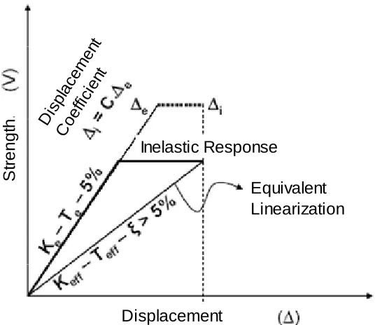
When a structure under seismic excitation is taken beyond its elastic limit, its maximum response is influenced by two phenomena: stiffness degradation and energy dissipation, as shown in Fig. (1.a). The degradation in stiffness is caused by yielding of sections in the structure and its primary effect is the increase of the displacement demand due to lengthening of the fundamental period. At the same time, the hysteretic behavior of the yielding sections results in energy dissipation, which reduces the displacement demand due to an increase of damping in the system. These effects can be visualized for different regions of the design spectrum in Fig. (1.b). If a Single Degree of Freedom (SDOF) system with initial period Tn

is considered of infinite strength and 5% damping, it responds with a peak elastic

displacement Δe. But, if a reduced strength is considered, yielding occurs, stiffness degrades,

period lengthens to Teff and displacement demand increases to Δ'e. However, this tendency to displace more is counteracted by the increase in damping that in turn, reduces the displacement demand to the final maximum inelastic displacement Δi. In a certain section of

(20)

7 Displacement

S

tr

e

ngt

h

.

Equivalent Linearization Inelastic Response

Dis pla

cem ent

Co effi

cie nt

Figure 2 - Linearization Methods

For design purposes, since seismic hazard is usually presented in the form of elastic spectra, it is convenient to substitute the real inelastic system for an elastic one such that both systems reach the same peak displacement. There are two widely known approaches to linearize inelastic SDOF systems: The Displacement Modification Method and the Equivalent Linearization Method.

Displacement Modification Method (DMM)

This method is used by AASHTO (Imbsen, 2007) and Caltrans (2006) to replace the inelastic system by an elastic one, with the same level of elastic-damping and fundamental-elastic period. The peak response of the substitute system is modified to match the peak displacement of the inelastic system by application of the displacement coefficient C (Fig. 2).

(21)

8 characteristic period, T*, equal to 1.25 times the period, Ts, at the end of the spectral acceleration plateau (Fig. 3). For short period structures, C is increased as given by Eq. 1 (Imbsen, 2007), where R equals the maximum ductility demand expected in the structure, and T* equals 1.25 Ts (Fig.3).

0 . 1 1 * 1 1

C= −

_⎟

+ ≥

⎠

⎞

⎜

⎝

⎛

R T T

R (Eq.1)

Equivalent Linearization Method (ELM)

This method is used in DDBD. In this approach, an inelastic SDOF is substituted by an elastic system with secant stiffness and equivalent viscous damping which, under earthquake excitation, reaches the same maximum displacement as the original inelastic SDOF (Fig.2) (Shibata and Sosen, 1976).

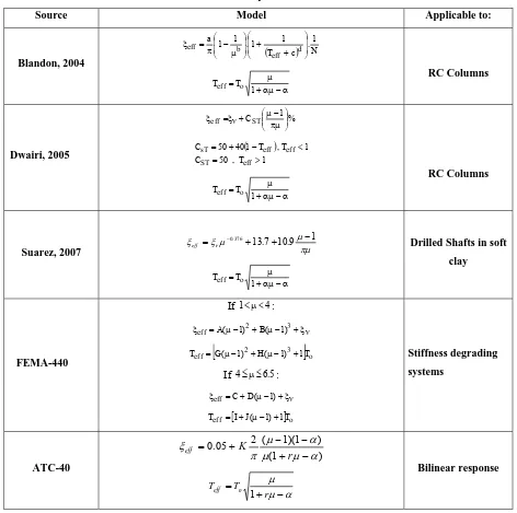
Several studies have been conducted to obtain models of equivalent damping, ξeq, for different types of structural elements such as RC beams, unbonded-postensioned walls, steel members, drilled shafts and piles and isolation/dissipation devices. (Dwairi, 2005 ; Blandon,

2004 ; Suarez, 2007 ) . Table 1 shows some of these models where ξv is the viscous damping in the elastic range, r Is the ratio between second and first slopes in a bilinear force-deformation response, μ is the ductility demand, Teff is the effective period that corresponds to secant stiffness and a,b,c,d, and A,B,C,D,G,H,I,J are coefficients that depend on the hysteresis model.

(22)

9 and Priestley (2004) and Suarez and Kowalsky (2007) to obtain models that can be used with DDBD.

Table 1 - Models for equivalent linearization

Source Model Applicable to:

Blandon, 2004

( ) N

1 . c T 1 1 . 1 1 a d eff b

eff _⎟⎟

⎠ ⎞ ⎜ ⎜ ⎝ ⎛ + + ⎟ ⎟ ⎠ ⎞ ⎜ ⎜ ⎝ ⎛ μ − π = ξ α − αμ + μ = 1 T

T_eff _o RC Columns

Dwairi, 2005

% 1 C_ST

eff=ξ + ⎜⎜_⎝⎛μ_πμ− ⎟⎟_⎠⎞ ξ _ν ( ) 1 T , 50 C 1 T , T 1 40 50 C eff ST eff eff sT > = < − + = α − αμ + μ = 1 T T_eff _o

RC Columns

Suarez, 2007 πμ

μ μ ξ ξ ν 1 9 . 10 7 . 13 376 .

0 ₊ ₊ −

= − eff α − αμ + μ = 1 T T_eff _o

Drilled Shafts in soft clay

FEMA-440

If 1<μ<4:

ν ξ + − μ + − μ =

ξ 2 3

eff A( 1) B( 1)

[

2 3

]

o

eff G( 1) H( 1) 1T

T = μ− + μ− +

If 4≤μ≤6.5:

ν ξ + − μ + =

ξeff C D( 1)

[ ]o

eff I J( 1) 1T

T = + μ− +

Stiffness degrading systems ATC-40 ) 1 ( ) 1 )( 1 ( 2 05 . 0 α μ μ α μ π ξ − + − − + = r K eff α μ μ − + = r T T_eff _o

1

Bilinear response

(23)

10 period based on stiffness which is not secant to maximum response. According to FEMA, using such definition of period reduces the variability in the determination of equivalent damping.

Comparative analysis of the linearization approaches

As it was mentioned before, the inelastic response of a SDOF system is affected by stiffness degradation and increased damping. The equivalent linearization approach, used in DDBD, accounts for these two phenomena in a rational and independent way. Conversely, with the displacement modification, these effects are mixed together, without considering the relation between damping and ductility and the energy dissipation characteristics of different materials. Furthermore, most of the research on coefficient C has been based on the response of elastic perfectly-plastic SDOF with mass proportional viscous damping, even though that type of response is not observed in reinforced concrete piers. (Priestley et al, 2007)

For a quantitative comparison of the two linearization methods, a displacement coefficient C is derived from an equivalent damping model. Based on its definition,

e Δ

i Δ

C= (Eq. 2)

where Δi is the inelastic displacement and Δe is the elastic displacement of a SDOF system

with the same fundamental period Tn and 5% viscous damping. Δi can be found in terms of

effective period Teff and equivalent damping ξeq as (Eurocode , 1998):

eff eff

eff ₂ _ξ

7 ) e(T Δ ) i(T Δ +

= _{(Eq. 3)}

Replacing Eq.3 in Eq.2, C is found as the ratio of elastic displacement for initial and effective periods times a damping reduction factor:

eff n eff ξ 2 7 ) e(T Δ ) e(T Δ C +

= _(Eq.4)

(24)

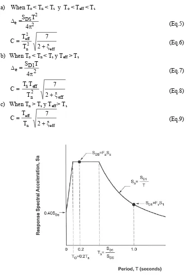
11 a) When To < Tn < Ts y To < Teff < Ts

2 2 DS e 4 T S π =

Δ _(Eq.5)

eff 2 n 2 eff ξ 2 7 T T C +

= _(Eq.6)

b) When To < Tn < Ts y Teff > Ts

2 1 D e 4 T S π =

Δ _(Eq.7)

eff 2 n eff ξ 2 7 T T s T C +

= _(Eq.8)

c) When Tn > Ts y Teff > Ts

eff n eff ξ 2 7 T T C +

= _(Eq.9)

(25)

12 Using Eq. 9, C has been found for SDOF systems with Tn > 1 s using the equivalent

linearization models presented in Table 1. The results are shown in Fig.4. Following an inverse approach, and also for the sake of comparison, the equal displacement approximation has been translated into an equivalent damping model, with results as shown in Fig. 5

0 0.2 0.4 0.6 0.8 1 1.2 1.4 1.6

1 2 3 4 5 6 7

Ductility D isp la ce m e n t C o ef f. C

Thin Takeda (Blandon) TYPE B (ATC 40)

RC Columns (Dwairi)

Equal Displacement

Degrading Stiff. (FEMA 440)

Drilled Shaft Hº A (Suarez)

Figure 4 - Equivalent damping models translated to displacement coefficient

0 5 10 15 20 25 30 35

0 1 2 3 4 5 6 7

Ductility E q ui va le nt D a m p in g ( % )

Thin Takeda (Blandon) TYPE B (ATC 40) RC Columns (Dwairi) Equal Displacement

Degrading Stiff (FEMA 440)" Drilled Shaft (Suarez)

(26)

13 It has been shown that for SDOF systems, equivalent linearization can be converted to displacement modification or vice versa, and as a result the two approaches are valid to linearize the inelastic response of SDOF systems. In addition, from observation of Figs. 4 and 5, important conclusions can be advanced:

• The equivalent damping models translate into displacement coefficient models that increase with ductility, whereas the equal displacement approximation implies C = 1, independently from ductility. Fig. 6 shows C coefficient from FEMA-440 (2006) as a function of Tn and the force reduction factor, R, which for elastoplastic response can

be assumed equal to ductility. This graph shows that in reality, C increases with ductility as predicted by the equivalent damping models. Assuming C = 1 seems to be a gross average of response.

Figure 6 - C coefficient for elastoplastic systems in sites class B. (FEMA, 2006)

(27)

14 ductility less than 2.5 and more damping for higher ductility. That means that bridge piers with ductility less than 2.5 require less strength if designed based on Dwairi or Blandon equivalent damping models.

• The equivalent damping model in FEMA 440 can not be compared to other damping models since this model is meant to be used with combination with an effective period that is not base on stiffness secant to maximum response.

• Fig. 5 shows that the equal displacement approximation is conservative for design of drilled shafts bents, since ignores soil damping.

4. DISPLACEMENT BASED DESIGN METHODS

4.1 Seismic Design Criteria by Caltrans

The Seismic Design Criteria (SDC) by Caltrans (2006) shifted towards displacement based design in 1999 consolidating ATC-32 recommendations (American Technology Council, 1996). The SDC is currently used for design of ordinary bridges in the state of California.

The SDC of Caltrans presents an iterative design procedure in which the lateral strength of the system (size and reinforcement of the substructure sections) is assumed at the beginning of the process. Then, by means of displacement demand analysis and displacement capacity verification, it is confirmed that the bridge with the assumed strength has an acceptable performance, otherwise, the strength is revised and the process repeated.

In the demand analysis, the peak inelastic displacement demands are estimated from a linear elastic response spectrum analysis of the bridge with cracked (secant to yield point) section stiffness. Then, elastic peak displacements are converted to peak inelastic displacements using the Displacement Modification Method described in Section 3.1.

(28)

15

4.2 Proposed AASHTO Guide Specification for LRFD Seismic Bridge

Design

The AASHTO LRFD Bridge Design Specifications (2004) and the AASHTO Standard Specifications are essentially the recommendations that were completed by the Applied Technology Council (ATC-6) in 1981 and adopted by AASHTO as a “Guide Specification” in 1983. Recognizing the availability of improvements since ATC-6 as documented in NCHRP 12-49, Caltrans Seismic Design Criteria (SDC) 2006, SCDOT – Seismic Design Specifications for Highway Bridges (2002) and related research projects, the T-3 AASHTO committee for seismic design started a project to update the LRFD guidelines that yielded the proposed AASHTO Guide Specification for LRFD Seismic Bridge Design (Imbsen, 2007).

The LRFD Seismic guide recognizes the variability of seismic hazard over the US territory and specifies different Seismic Design Categories. For category A no design is required, for categories B, C and D, demand analysis and capacity verification is required. The design procedure is in concept similar to the procedure by Caltrans, described in the previous section. For regular bridges, the demand analysis is performed by the uniform load method for regular bridges, while the spectral modal analysis can be used for all bridges. The capacity verification can be done using implicit equations for seismic design category B or C and by pushover analysis for categories D. As in Caltrans SDC, and with the exception of seismic category A, the proposed guide requires the application of capacity design principles for the detailing of the substructure sections and protected elements.

4.3 Direct Displacement Based Design

(29)

16 1) Determination of a target displacement profile for the bridge.

2) Evaluation of a substitute SDOF system, including the determination of equivalent damping based on ductility demand at target displacement.

3) Determination of required stiffness and strength using displacement design spectra. 4) Distribution of strength and application of capacity design principles.

DDBD requires no iteration when the target displacement profile can be accurately estimated at the beginning of the process. That is the case when a continuous bridge is designed in the longitudinal direction. No iteration is neither required for transverse design when the superstructure is formed by simply supported spans or when the superstructure displaces transversely as a rigid body. The DDBD method for bridges is covered in detail in Part II.

5. RESEARCH OBJECTIVES

The main objective of this research is to bridge the gap between existing research DDBD and its implementation for design of conventional highway bridges, with all their inherent complexities.

Since it was first proposed by Priestley in 1993, DDBD has been under constant development. Despite the important and extensive progress of DDBD in the last decade, several items require specific attention to fully implement DDBD for conventional highway bridges. The specific objectives of this dissertation are:

• Determine under what conditions predefined displacement patterns can be used for DDBD of different types of bridges.

• Propose a model for determination of a stability-based target displacement for piers.

• Propose models to account for: displacement capacity of the superstructure and skew.

• Define a general DDBD procedure for conventional highway bridges

• Determine the scope and applicability of DDBD

(30)

17

• Develop software for the application of DDBD

6. REFERENCES

AASHTO, 2004, LRFD Bridge design specifications, fourth edition, American Association of State Highway and Transportation Officials, Washington, D.C.

ATC, 2003, NCHRP 12-49 Recommended LRFD Guidelines for the Seismic Design of Highway Bridges, http://www.ATCouncil.org, (accessed June, 2008)

ATC-40. "Seismic Evaluation and Retrofit of Concrete Buildings/Volume 1". 1996,

http://www.ATCouncil.org, (accessed June, 2008)

Blandon Uribe C., Priestley M. 2005, Equivalent viscous damping equations for direct displacement based design, "Journal of Earthquake Engineering", Imperial College Press, London, England, 9, SP2, pp.257-278.

Caltrans, 2006, Seismic Design Criteria, Caltrans, http://www.dot.ca.gov/hq/esc/

earthquake_engineering, (accessed April 18, 2008)

Calvi G.M. and Kingsley G.R., 1995, Displacement based seismic design of multi-degree-of-freedom bridge structures, Earthquake Engineering and Structural Dynamics 24, 1247-1266.

Dwairi, H. and Kowalsky, M.J., 2006, Implementation of Inelastic Displacement Patterns in Direct Displacement-Based Design of Continuous Bridge Structures, Earthquake Spectra, Volume 22, Issue 3, pp. 631-662

Dwairi, H., 2004. Equivalent Damping in Support of Direct Displacement - Based Design with Applications To Multi - Span Bridges. PhD Dissertation, North Carolina State University

EuroCode 8, 1998, Structures in seismic regions – Design. Part 1, General and Building”, Commission of European Communities, Report EUR 8849 EN

FEMA, 2006. "FEMA 440, Improvement Of Nonlinear Static Seismic Analysis Procedures",

(31)

18 Imbsen, 2007, AASHTO Guide Specifications for LRFD Seismic Bridge Design, AASHTO,

http://cms.transportation.org/?siteid=34&pageid=1800, (accessed April 18, 2008).

Kowalsky M.J., 2002, A Displacement-based approach for the seismic design of continuous concrete bridges, Earthquake Engineering and Structural Dynamics 31, pp. 719-747. Kowalsky M.J., Priestley M.J.N. and MacRae G.A. 1995. Displacement-based Design of RC

Bridge Columns in Seismic Regions, Earthquake Engineering and Structural Dynamics 24, 1623-1643.

Miranda E. Inelastic displacement ratios for structures on Brm sites. Journal of Structural Engineering 2000; 126:1150–1159.

Newmark NM, Hall WJ. Earthquake Spectra and Design. Earthquake Engineering Research Institute, Berkeley, CA, 1982.

Ortiz, J., 2006, Displacement-Based Design of Continuous Concrete Bridges under Transverse Seismic Excitation". European School for Advanced Studies in Reduction of Seismic Risk (ROSE School).

Priestley, M. J. N., 1993, Myths and fallacies in earthquake engineering-conflicts between design and reality, Bulletin of the New Zealand Society of Earthquake Engineering, 26 (3), pp. 329–341

Priestley, M. J. N., Calvi, G. M. and Kowalsky, M. J., 2007, Direct Displacement-Based Seismic Design of Structures, Pavia, IUSS Press

Shibata A. and Sozen M. Substitute structure method for seismic design in R/C. Journal of the Structural Division, ASCE 1976; 102(ST1): 1-18.

South Carolina Department of Transportation (2002), Seismic Design Specifications for Highway Bridges, First Edition 2001, with October 2002 Interim Revisions

(32)

19

PART II

IMPLEMENTATION OF THE DIRECT

DISPLACEMENT-BASED DESIGN METHOD FOR SEISMIC DESIGN OF

HIGHWAY BRIDGES

Vinicio A. Suarez and Mervyn J. Kowalsky

Department of Civil, Construction and Environmental Engineering, North Carolina State University, Campus-Box 7908, Raleigh, NC-27695, USA

ABSTRACT

(33)

20

1. INTRODUCTION

After the Loma Prieta earthquake in 1989, extensive research has been conducted to develop improved seismic design criteria for bridges, emphasizing the use of displacements rather than forces as a measure of earthquake demand and damage in bridges. (Priestley, 1993; ATC, 1996; Caltrans, 2006; ATC, 2003; Imbsen, 2007)

Several Displacement Based Design (DBD) methodologies have been proposed. Among them, the Direct Displacement-Based Design Method (DDBD) (Priestley, 1993) has proven to be effective for performance-based seismic design of bridges, buildings and other types of structures (Priestley et al, 2007). Specific research on DDBD of bridges has focused on design of bridge piers (Kowalsky, 1995), drilled shaft bents with soil-structure interaction (Suarez and Kowalsky, 2007) and multi-span continuous bridges (Calvi and Kingsley, 1997; Kowalsky 2002; Dwairi, 2005; Ortiz, 2006).

DDBD differs from other DBD procedures for bridges, such as the Seismic Design Criteria of Caltrans (2005) or the newly proposed AASHTO Guide Specification for LRFD Seismic Bridge Design (Imbsen, 2007), in the use of an equivalent linearization approach and in its execution. While the other methods are iterative and require strength to be assumed at the beginning of the process, DDBD directly returns the strength required by the structure to meet a predefined target performance.

The purpose of this report is to present the DDBD method with all the details required for its application to the design of conventional highway bridges. The method presented here includes new features such as: the incorporation of the displacement capacity of the superstructure as a design parameter, the determination of a stability-based target displacement for piers, the design of skewed bents and abutments, among others.

2. FUNDAMENTALS OF DDBD

(34)

21 displacement and returns the strength required to meet the target displacement under the design earthquake. The target displacement can be selected on the basis of material strains, drift or displacement ductility, either of which is correlated to a desired damage level or limit state. For example, in the case of a bridge column, designing for a serviceability limit state could imply steel strains to minimize residual crack widths that require repair or concrete compression strains consistent with incipient crushing.

DDBD uses an equivalent linearization approach (Shibata and Sozen, 1976) by which, a nonlinear system at maximum response, is substituted by an equivalent elastic system. This system has secant stiffness, Keff, and equivalent viscous damping, ξeq, to match the maximum response of the nonlinear system (Fig 1). In the case of multi degree of freedom systems, the equivalent system is a Single Degree of Freedom (SDOF) with a generalized displacement, Δsys, and the effective mass, MEFF, computed with Eq. 1 and Eq. 2 respectively (Fig.2) (Calvi and Kingsley, 1995). In these equations, Δ1….Δi…Δn are the displacements of the piers and abutments (if present) according to the assumed displacement profile, and M1….Mi….Mn are effective masses lumped at the location of piers and abutments (if present).

(35)

22

Figure 2 - Equivalent single degree of system.

∑

= = = = Δ Δ =

Δ _i _n

i i i n i i i i sys M M 1 1 2 (1)

∑

= = = = Δ ⎟ ⎠ ⎞ ⎜ ⎝ ⎛ _Δ

= _i _n

i i i n i i i i eff M M M 1 2 2 1 (2)

(36)

23 that form the earthquake resisting system, and the elements are designed and detailed following capacity design principles to avoid the formation of unwanted mechanisms.

Figure 3 – Determination of effective period in DDBD

2.1 Equivalent damping

Several studies have been performed to obtain equivalent damping models suitable for DDBD (Dwairi 2005, Blandon 2005, Suarez 2006, Priestley et al 2007). These models relate equivalent damping to displacement ductility in the structure.

For reinforced concrete columns supported on rigid foundations, ξeq, is computed with Eq. 3 (Priestley, 2007).

t t

eq πμ

μ

(37)

24 For extended drilled shaft bents embedded in soft soils, the equivalent damping is computed by combination of hysteretic damping, ξeq,h, and tangent stiffness proportional viscous damping, ξv, with Eq. 4 (Priestley and Grant, 2005). The hysteretic damping is computed with Eq. 5 as a function of the ductility in the drilled shaft. The values of the parameters p

and q are given in Table 1 for different types of soils and boundary conditions (Suarez 2005). In Table 1, clay-20 and clay-40 refer to saturated clay soils with shear strengths of 20 kPa and 40 kPa respectively. Sand-30 and Sand-37 refer to saturated sand with friction angles of 30 and 37 degrees respectively. A fixed head implies that the head of the extended drilled shaft displaces laterally without rotation, causing double bending in the element. A pinned head implies lateral displacement with rotation and single bending. To use Eq. 4, ξv should be taken as 5%, since this value is typically used as default to develop design spectra.

h eq v

eq ,

378 .

0 ξ

μ ξ

ξ = − +

μ ≥1 (Eq. 4)

μ μ ξ_eq_,_h = p+q −1

μ ≥1 (Eq. 5)

Table 1. Parameters for hysteretic damping models in drilled shaft - soil systems

(38)

25 cases where the target displacement is less than the yield displacement of the element, a linear relation between damping and ductility is appropriate. Such relation is given by Eq. 6.

μ ξ ξ

ξ_eq = _v +(q− _v)

μ <1 (Eq. 6)

Figure 4. Equivalent damping models for bridge piers

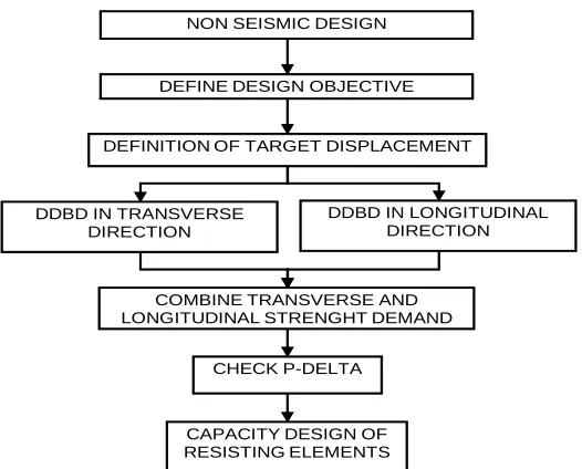
3. GENERAL DDBD PROCEDURE FOR BRIDGES

(39)

26

NON SEISMIC DESIGN

DEFINE DESIGN OBJECTIVE

DEFINITION OF TARGET DISPLACEMENT

COMBINE TRANSVERSE AND LONGITUDINAL STRENGHT DEMAND

CHECK P-DELTA DDBD IN TRANSVERSE

DIRECTION

DDBD IN LONGITUDINAL DIRECTION

CAPACITY DESIGN OF RESISTING ELEMENTS

Figure 5 - DDBD main steps flowchart

DDBD IN TRANSVERSE AND LONGITUDINAL DIRECTION FMS

EMS

DEFINE DISPLACEMENT PATTERN

SCALE PATTERN TO REACH TARGET DISPLACEMENT

COMPUTE DUCTILITY DEMAND AND EQUIVALENT DAMPING

COMPUTE SYSTEM MASS, DISPLACEMENT AND EQUIVALENT DAMPING

DETERMINE EFFECTIVE PERIOD, STIFFNESS AND REQUIRED STRENGTH

BUILT 2D MODEL WITH SECANT MEMBER STIFFNESS

COMPUTE DESIGN FORCES

Is the strenght distribution correct?

FMS EMS

COMPUTE INERTIAL FORCES FIND REFINED FIRST MODE SHAPE BY STATIC ANALYSIS

USE FIRST MODE SHAPE AS DISPLACEMENT PATTERN

BUILT 2D MODEL WITH SECANT MEMBER STIFFNESS

PERFORM EFFECTIVE MODE SHAPE ANALISYS

USE COMBINED MODAL SHAPE AS DISPLACEMENT PATTERN

Was the displacement Pattern predefined?

YES

NO NO

YES

(40)

27 The flowcharts in Fig. 6 show the procedure for DDBD in the transverse and longitudinal

direction, as part of the general procedure shown in Fig. 5. As seen in Fig. 6, there are three

variations of the procedure: (1) If the displacement pattern is known and predefined, DDBD is

applied directly; (2) If the pattern is unknown but dominated by the first mode of vibration, as in

the case of bridges with integral or other type of strong abutment, a First Mode Shape (FMS)

iterative algorithm is applied; (3) If the pattern is unknown but dominated by modal combination,

an Effective Mode Shape (EMS) iterative algorithm is applied. The direct application of DDBD,

when the displacement pattern is known, requires less effort than the application of the FMS or

EMS algorithms. Recent research by the author (Suarez and Kowalsky, 2008a) showed that

predefined displacement patterns can be effectively used for design of bridge frames, bridges

with seat-type of other type of weak abutments and bridges with one or two expansion joints.

These bridges must have a balanced distribution of mass and stiffness, according to AASHTO

(Ibsen, 2007). A summary of the design algorithms applicable to common types of highway

bridges is presented in Table 2.

Table 2. Displacement patterns for DDDBD of bridges

(41)

28

3.1 Design Objective

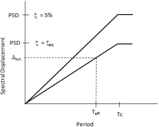
In DDBD, a design objective or performance objective is defined by specification of the seismic hazard and the design limit state to be met under the specified seismic hazard. The seismic hazard is represented by an elastic displacement design spectrum (Fig 3). The design spectrum is characterized by a Peak Spectral Displacement, PSD, and a corner period, Tc. The design limit state can be based on material strain limits, ductility, drift or any other damage or stability index. DDBD allows any combination of seismic hazard and design limit state; therefore, it can be used as a tool for Performance Based Seismic Engineering. Some of the most common design limit states are:

Life safety

This limit is used in the AASHTO Guide Specifications for LRFD Seismic Bridge Design (Imbsen, 2007) for bridges in Seismic Design Category (SDC) “D”. It is intended to protect human life during and after a rare earthquake. This limit implies that the bridge has low probability of collapse but may suffer significant damage in piers and partial or complete replacement may be required. To compute pier displacements to meet the life safety limit the ductility limits proposed in the AASHTO LRFD Guides (Imbsen, 2007) can be used. For single column bents ductility equals five. For multiple column bents, ductility equals six. For pier walls is the weak direction, ductility equals five. For pier walls in the strong direction, ductility equals one.

Damage control.

(42)

29 Specific values of compression strain for the confined concrete can be estimated using the energy balance approach developed by Mander (1988). In this model (Eq. 7), the damage-control concrete strain, εc,dc, is a function of volumetric transverse steel ratio, ρv , yield stress of the transverse steel reinforcement, fyh, ultimate strain of the transverse steel reinforcement , εsu,, compressive strength of the confined concrete, f’cc,(Eq. 8) compressive strength of the unconfined concrete, f’c, and the confinement stress f1 (Eq. 9).

` , ' 4 . 1 004 . 0 cc su yh v dc c f f ε ρ

ε = + (Eq. 7)

⎟ ⎟ ⎠ ⎞ ⎜ ⎜ ⎝ ⎛ − − +

= 1.254

' 2 ' 94 . 7 1 254 . 2 '

' 1 1

c c c cc f f f f f

f (Eq. 8)

yh vf

f₁ =0.5ρ (Eq. 9)

The damage control displacement for single column or multiple column bents can then be computed based on the damage control strains using the plastic hinge method (Priestley and Calvi, 1993). This method is covered in Section 3.2.4.

Serviceability

This limit is more restrictive than the damage control limit state. It sets the limit beyond which damage in piers needs repair (Kowalsky, 2000). For circular reinforced concrete columns, typical strains related to this limit state are 0.004 for concrete in compression and 0.015 for steel in tension. The steel tension strain is defined as the strain at which residual cracks widths would exceed 1 mm. Serviceability pier displacement can be computed with the plastic hinge method covered in Section 3.2.4.

Stability limit

(43)

30 effects can be neglected in the design of piers when the stability index is less that 25%. For application in DDBD, Priestley et al (2007) suggest that if the stability index is higher that 8%, P-Δ effects should be counteract by an increase in the strength of the pier. However, stability index should not exceed 30%.

3.2 Determination of target displacement

Perhaps the most important step of the DDBD procedure is to determine the target displacement profiles in the transverse and longitudinal directions of the bridge. This process is executed in two steps: (1) Target displacements are computed for all earthquake resisting elements; (2) Target profiles for transverse and longitudinal response are proposed so that one or more elements meet their target displacements. No element must exceed its target displacement. The proposed target profiles must be consistent with the expected dynamic response of the bridge. Therefore in most cases, it will not be possible that all elements meet their target displacements and there will be one or two elements controlling the displacement profiles of the bridge. A detailed explanation on how to determine the target displacements for superstructures, abutments and piers, and the target displacement profiles for a bridge is presented next.

3.2.1 Plan Curvature

(44)

31

Figure 7. Curve bridge unwrapped to be designed as straight

A practical solution suggest that bridges with subtended angles of 90 degrees or less can be unwrapped and designed as straight bridges (Fig. 7). This is currently recommended in other bridge design codes (Caltrans, 2004; Ibsen 2007). Span lengths and skew angles in the equivalent straight bridge must be the same as in the curved bridge. Gravity induced forces, especially those resulting from the curved geometry, must be carefully considered and combined with seismic actions. (see Section 3.8.1).

3.2.2 Superstructure target displacement

It is a common strategy to design bridges in which damage and energy dissipation take place in the piers and abutments while the superstructure is protected and designed to remain elastic. The reason is that the substructure elements can be effectively designed to be ductile and dissipate energy while most superstructures cannot.

(45)

32 If a target displacement is determined for the superstructure, this should meet the serviceability or other more restrictive strain limits or should by controlled by the displacement capacity of expansion joints. This discussion applies only to DDBD of bridges in the transverse direction. Bridge superstructures are usually stiff and strong in their axis, so their performance is not an issue when designing in the longitudinal direction.

Determining a superstructure target displacement is important for design of bridges responding with a flexible transverse displacement pattern, including: bridges with strong abutments, bridges with weak and flexible superstructures, bridges with unbalanced mass and stiffness.

The DDBD framework allows easy inclusion of superstructure transverse target displacement into the design procedure. The transverse target displacement profile of the bridge must be defined accounting for the target displacement of the piers, abutments and target displacement of the superstructure.

The determination of a target displacement for the superstructure requires moment curvature analysis of the superstructure section and double integration of the curvature profile along the length of the superstructure. Moment curvature analysis should account for expected material properties and strains caused by gravity loads. The result of the moment curvature analysis is the target curvature to meet the specified strain limits. Other important result is the flexural stiffness of the superstructure, which is also needed in design.

If it is believed that the target displacement of the superstructure should be controlled by yielding of the longitudinal reinforcement of a concrete deck, a yield curvature as target curvature can be estimated with Eq. 10. Where ws is the width of the concrete deck and εy is the yield strain of the steel reinforcement. The yield curvature of a section in mainly dependent on its geometry and it is insensitive to its strength and stiffness (Priestley, 2007).

s y ys

w

ε

(46)

33

Figure 8 - Assumed superstructure displacement pattern

Assuming that the superstructure responds in the transverse direction as a simply supported beam, with the seismic force acting as a uniform load (Fig. 8), the curvature along the superstructure, φs(x), as a function of the target curvature of the superstructure, φsT, is given by Eq. 11. Double integration of the curvature function results in the target displacement function shown as Eq. 12. Where Ls is the length of the superstructure and x is the location of the point of interest.

2 2 ) ( 4 4 s ys s ys x s L x L x φ φ

φ = − (Eq. 11)

⎥ ⎥ ⎦ ⎤ ⎢ ⎢ ⎣ ⎡ ₋ ₊ = Δ ₂ 3 3 4 6 2 4 2 s s s Ts Ts L x L x L x

φ (Eq. 12)

Eq. 12 gives the target displacement relative to the abutments. However, since the abutments are also likely to displace, Eq. 13 should be added to Eq. 12 to obtain a total target displacement. In Eq. 13, Δ1 and Δn are the displacements of the initial and end abutment respectively. x L_s n A 1 1 Δ − Δ + Δ =

Δ (Eq. 13)

i s n s i s i s i Ts Tsi x L L x L x L x ₁ 1 2 3 3 4 6 2 4

2 Δ −Δ

+ Δ + ⎥ ⎥ ⎦ ⎤ ⎢ ⎢ ⎣ ⎡ ₋ ₊ =

Δ φ (Eq. 14)

(47)

34 then ΔTsi controls design and becomes the design target displacement for the pier. An example that illustrates the application of this model is presented in Section 5.1

3.2.3 Abutment target displacement

Due to specific configurations and design details, an appropriate estimation of lateral target displacement will in most cases require a nonlinear static analysis of the abutment that has been previously designed for non-seismic loads. Instead of such analysis, a gross estimation of the displacement that will fully develop the strength of the fill behind the back or wing walls can be obtained with Eq. 15 (Imbsen, 2008). In this equation, fh is a factor taken as 0.01 to 0.05 for soils ranging from dense sand to compacted clays and Hw is the height of the wall. This relation might be useful in the assessment of a target displacement for integral abutments or seat-type abutments with knock-off walls.

w h T = f H

Δ (Eq. 15)

Table 3 - Parameters for DDBD of common types of piers

Transv. Long. Transv. Long. Transv. Long.

Single column integral bent H+Hsup+Lsp H+2Lsp 1/3 1/6 Hp Hp/2

Single extended drilled shaft integrall bent Le+Hsup Le+Lsp varies varies Hp Hp/2

Single column non-integral bent pinned in long direction H+Hsup+Lsp H+Lsp 1/3 1/3 Hp Hp

Single extended-drilled-shaft non-integral bent pinned in

long direction Le+Hsup Le varies varies Hp Hp/2

Multi column integral bent H+2Lsp H+2Lsp 1/6 1/6 Hp/2 Hp/2

Multi extended-drilled-shaft integrall bent Le+Lsp Le+Lsp varies varies Hp/2 Hp/2

Multi column integral bent with pinned base H+Lsp H+Lsp 1/3 1/3 Hp Hp

Multi column bent pinned in longitudinal direction H+2Lsp * H+Lsp * 1/6 * 1/3 * Hp/2 * Hp * Multi extended-drilled-shaft non-integral bent pinned in

long direction Le * Le * varies * varies * Hp/2 * Hp *

* These are in-plane and out-of-plane values and must be corrected for skew to get transverse and longitudinal values Effective Height Hp Yield Disp. Factor α

PIER TYPE Shear Height Hs

3.2.4 Pier target displacement

(48)

35 can be established. The first requirement is usually easy to comply knowing that the relation between strain in the plastic hinge region and displacement at the top of a pier is independent from the strength and stiffness of the pier.

The second item requires an assessment of design ductility and the use of an existing ductility-damping model such as those presented in Section 2.1. The determination of ductility demand requires knowledge of yield displacement which is calculated as part of the target displacement determination. As a result of this, the design of most common types of piers used in highway bridges can be easily implemented in DDBD. This includes piers with isolation/dissipation devices and piers with soil-structure interaction.

A graphic description of common types of reinforced concrete piers used in conventional bridges is presented in Fig. 9. In relation to that figure, Table 3 shows values for: the effective height of the pier Hp, yield displacement factor α, and shear height Hs.

These parameters are given for design in transverse and longitudinal axes of the bridge. In Table 3, H is the height of column, Le is the effective height of drilled shaft, Hsup is the height from the soffit to the centroid of the superstructure and Lsp is the strain penetration length. The parameters Le and α for drilled shaft bents are shown in Fig. 10 in terms of the type of soil, above ground height of the bent, La, and diameter of the drilled shaft section D. Plastic Hinge Method

Strain-based target displacements are determined using the plastic hinge method (Priestley et al, 2007). For any type of pier listed in Table 3, the target displacement, Δt, along the transverse and longitudinal axis of the bridge is estimated with Eq. 16. In this equation, Δy is the yield displacement of the pier, φt and φy are the target and yield curvature respectively, Lp is the plastic hinge length and Hp is the effective height of the pier defined in Table 3.

(

t y

)

p p y

T =Δ + φ −φ L H

(49)

36

(50)

37

Figure 10 - Le and a for definition of the equivalent model for drilled shaft bents (Suarez and Kowalsky, 2007)

The target curvature is determined in terms of the target concrete strain, εc,T, target steel strain, εs,T, and neutral axis depth, c, with Eq. 17. The target curvature can be controlled by the concrete reaching its target strain in compression or the flexural reinforcement reaching its target strain in tension.

⎥ ⎦ ⎤ ⎢

⎣ ⎡

− =

c D c

T s T c dc

,

, ,

min ε ε

(51)

38 The neutral axis depth can be estimated with Eq. 18, where P is the axial load acting on the element and Ag is the gross area of the section (Priestley et al, 2007)

⎟ ⎟ ⎠ ⎞ ⎜ ⎜ ⎝ ⎛ + = g ce A f P D c ' 25 . 3 1 2 .

0 (Eq. 18)

The yield curvature φy is independent of the strength of the section and can be determined in terms of the yield strain of the flexural reinforcement εy and the diameter of the section D with in Eq. 19 (Priestley et al, 2007)

D

y y

ε

φ =2.25 (Eq. 19)

The yield displacement Δy is given by Eq. 20, where α is given in Table 3 for transverse and longitudinal directions. For extended drilled shaft bents, α is shown in Figure 10.

( )

2

p y y =αφ H

Δ (Eq. 20)

Life safety target displacement

Is computed introducing the ductility limits given in Section 3.1 in Eq. 21. μ

y T =Δ

Δ (Eq. 21)

Damage control target displacement

(52)

39 Serviceability target displacement

The strain limits in Section 3.1 are used to compute a target curvature and then a target displacement with Eq. 16

Target displacements for SDC “B” and “C”

For these SDCs, the equations given in AASHTO (Ibsen, 2007) for the assessment of displacement capacity for moderate plastic action (Eq. 23) and minimal plastic action (Eq. 24) can also be used in DDBD to get a target displacement. In Eq. 23 and Eq. 24, Hc is the clear height of the columns and Λ is 1 for columns in single bending and 2 for columns in double bending. c c c c H H D

H 2.32ln 1.22 0.003

003 .

0 _⎟⎟≥

⎠ ⎞ ⎜ ⎜ ⎝ ⎛ − ⎟⎟ ⎠ ⎞ ⎜⎜ ⎝ ⎛ Λ − =

Δ (m) (Eq. 23)

c c c c H H D

H 1.27ln 0.32 0.003

003 .

0 _⎟⎟≥

⎠ ⎞ ⎜ ⎜ ⎝ ⎛ − ⎟⎟ ⎠ ⎞ ⎜⎜ ⎝ ⎛ Λ − =

Δ (m) (Eq. 24)

Stability-based target displacement

A target displacement for a bridge pier to meet a predefined value of the stability index, θs, can be estimated with Eq. 25 (Suarez and Kowalsky 2008b), where the parameters a, b, c and

d are given in Tables 4 and 5 for piers on rigid foundations and extended drilled shaft bents in different types of soils. Table 4 gives the parameters for near fault sites and Table 5 for far fault sites. The parameter C in Eq. 25 is computed with Eq. 26 in terms of the peak spectral displacement, PSD, the corner period, Tc, the axial load acting on the pier, P, the effective mass on the pier, Meff , and the height of the pier H.

C d C c bC a s − + + = θ

(53)

40

H M

P PSD

T C

eff s y c

θ π

2 Δ

= (Eq. 26)

If a bridge pier is designed as a stand-alone structure, Meff can be computed taking a tributary area of superstructure and adding the mass of the cap-beam and a portion of the mass of the pier itself (1/3 is appropriate). If the target displacement is being determined for a pier that is part of a continuous bridge, Meff is computed with Eq. 27 as a fraction of the effective mass of the bridge, MEFF. The effective mass of the bridge is computed as with Eq. 2 and vi is computed with Eq.31

EFF i eff v M

M = (Eq. 27)

Table 4 - Parameters to define Eq.15 for far fault sites

Table 5 - Parameters to define Eq.15 for near fault sites