INVESTIGATION
Stickbreaking: A Novel Fitness Landscape Model
That Harbors Epistasis and Is Consistent with
Commonly Observed Patterns of Adaptive Evolution
Anna C. Nagel,* Paul Joyce,†,‡Holly A. Wichman,* and Craig R. Miller*,†,1
*Department of Biological Sciences,†Department of Mathematics, and‡Department of Statistics, University of Idaho, Moscow, Idaho 83843
ABSTRACTIn relating genotypes tofitness, models of adaptation need to both be computationally tractable and qualitatively match observed data. One reason that tractability is not a trivial problem comes from a combinatoric problem whereby no matter in what order a set of mutations occurs, it must yield the same fitness. We refer to this as thebookkeeping problem. Because of their commutative property, the simple additive and multiplicative models naturally solve the bookkeeping problem. However, thefitness trajectories and epistatic patterns they predict are inconsistent with the patterns commonly observed in experimental evolution. This motivates us to propose a new and equally simple model that we callstickbreaking. Under the stickbreaking model, the intrinsicfitness effects of mutations scale by the distance of the current background to a hypothesized boundary. We use simulations and theoretical analyses to explore the basic properties of the stickbreaking model such asfitness trajectories, the distribution offitness achieved, and epistasis. Stickbreaking is compared to the additive and multiplicative models. We conclude that the stickbreaking model is qualitatively consistent with several commonly observed patterns of adaptive evolution.
A
DAPTIVE evolution is challenging to understand be-cause it depends on a rich array of biological properties. Among those receiving recent theoretical and experimental attention are the magnitude and distribution of mutationalfitness effects, the length of adaptive walks, the rate offitness increase, and the population dynamics that drive it (e.g., Gerrish and Lenski 1998; de Visser et al. 1999; Orr 2002, 2003; Rozenet al.2002; Cowperthwaiteet al.2005; Barrett et al. 2006; Desai et al. 2007; Eyre-Walker and Keightley 2007; Joyce et al. 2008; Rokyta et al. 2008; Barrick et al. 2009; Betancourt 2009; Burch and Chao 1999; Kryazhim-skiy et al.2009; Schoustraet al. 2009). Equally important are epistasis, pleiotropy, parallelism, mutation order, and the number of beneficial mutations available (e.g., Wichman et al. 1999, 2005; Holder and Bull 2001; Kim and Orr 2005; Weinreich et al. 2006; Silanderet al. 2007; Rokyta et al.2009, 2011; Chouet al.2011; Khanet al.2011; Kvitek and Sherlock 2011; Milleret al.2011). Note that the latter
features of adaptation are more meaningful when the iden-tities of the mutations are known and when we consider adaptation as a process subject to replication. For example, epistasis occurs when specific mutations have different ef-fects on different genetic backgrounds (Bonhoeffer et al. 2004; Sanjuánet al.2004). The rise of genomic sequencing technologies is having a dramatic effect on the ability of researchers to know the identity of mutations occurring dur-ing adaptation.
Knowing the identities of adaptive mutations expands the types of questions that can be addressed, but also creates new challenges. All models of adaptation must assignfitness values to genotypes that have arisen through mutation. In connecting genotype and fitness, a model must have the following property: if the wild-type background acquires mutations A1, A2, and A3 to yield a genotype with fitness w1,2,3, every possible order of these mutations must also result in fitness w1,2,3. As the number of fixed mutations grows, the number of possible pathways grows in a factorial manner. We call this consistency requirement the bookkeep-ing problem.
At least two groups of population genetic models address the bookkeeping problem: one maps genotype change (i.e.,
Copyright © 2012 by the Genetics Society of America doi: 10.1534/genetics.111.132134
Manuscript received June 28, 2011; accepted for publication October 28, 2011
1Corresponding author: Department of Mathematics, 300 Brink Hall, P.O. Box 441103,
mutation) directly ontofitness (GF models), and the second maps genotype onto phenotype and then phenotype onto
fitness (GPF models). Here we focus on the simpler GF models. Among these, theadditive modelassumes mutations have an additive effect on fitness. To be more precise, the
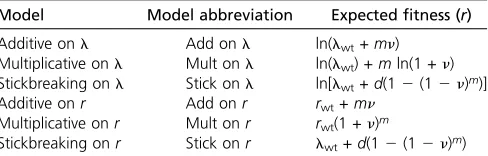
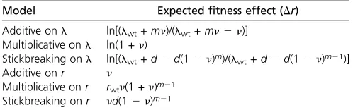
fitness after mutations A1 and A2 occur on the wild-type background is w1,2=wwt+Dw1 +Dw2, where Dw1 and Dw2are the intrinsic effects expressed asfitness differences of mutationsA1andA2. The bookkeeping problem is solved by the commutative property of addition (i.e.,Dw1+Dw2= Dw2 + Dw1). Under the multiplicative model, the intrinsic effects are selection coefficients affectingfitness in a multi-plicative fashion:w1,2=wwt(1 +s1)(1 +s2), wheres1and s2 are the intrinsic effects of mutations A1 and A2. Multi-plication also has the same commutative property [i.e., (1 + s1)(1 + s2) = (1 + s2)(1 + s1)] and thus solves the bookkeeping problem. Both of these solutions to the bookkeeping problem are simple to simulate and test on real data.
Another solution, implicit in the uncorrelated landscape model (Gillespie 1991; Orr 2002; Joyce et al. 2008), is to assume that the set of mutations arising in an adaptive walk can arise in only one order because each mutation is
bene-ficial on exactly one background. This occurs because the probability of a mutation being beneficial on more than one highly fit background is small enough to be ignored. Thus under the uncorrelated model, once replicate adaptive walks depart from each other, they are 100% divergent. Since the bookkeeping problem involves convergence, the bookkeep-ing problem is avoided. However, the uncorrelated model makes the extreme prediction for real data that no mutation will be beneficial on two different backgrounds.
Another set of models that avoids the bookkeeping problem is those that assume the number of beneficial mutations on any background is effectively infinite. Under this assumption, the probability of convergent evolution is zero and the bookkeeping problem does not arise. Examples of models that make this assumption include Gerrish and Lenski (1998), Rozenet al.(2002), Desaiet al.(2007), and Kryazhimskiyet al.(2009).
The NK model (Kauffman 1993) is unusual among GF models in that it can produce landscapes with intermediate levels of epistasis. In theNKmodel,Nis the number of sites andKis the number of other sites each site interacts with. WhenK= 0, it is the additive model and whenK=N21 it is equivalent to the uncorrelated model. When 0,K,N21, the interaction terms mean that the mutational effects are no longer background independent. The interactions bring more biological realism and allow richer patterns of epista-sis, but at the expense of model simplicity. Simulating data when 0 , K , N 2 1, while ensuring the bookkeeping criteria are met, is computationally challenging because it requires assigning fitnesses to the entirefitness landscape. The interactions also pose a problem for analyzing real data because they introduce a large number of parameters that must be estimated.
Kryazhimskiyet al.(2009) have also developed aflexible GF modeling framework where the uncorrelated and addi-tive models arise as special cases. These models allow dif-ferent types of epistasis and deceleratingfitness trajectories to be produced. However, because the fitness of beneficial mutations in such models depends only on the current fi t-ness, they do not solve the bookkeeping problem.
Thus there is an array of GF models. Among those that offer simple solutions to the bookkeeping problem (additive, multiplicative, and uncorrelated), they generally fail to predict several commonly observed properties of real adaptation. Specifically, in laboratory adaptations parallel evolution is not uncommon, mostfitness gain occurs early in a walk, and epistasis is common (Lenski and Travisano 1994; Bull et al. 1997; Elena and Lenski 1997; Wichman et al. 1999, 2005; Cooper and Lenski 2000; Burch et al. 2003; Sanjuán et al. 2004; Cowperthwaite et al. 2005; Woods et al. 2006; Barrick et al. 2009; Betancourt 2009; Rokyta et al. 2009, 2011; Chou et al. 2011; Khan et al. 2011).
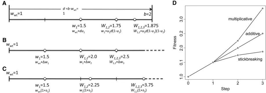
This leads us to propose a novel GF model for combining mutational effects that we call stickbreaking. The stickbreak-ing model is premised on the familiar idea that mutations have intrinsic effects. But rather than assuming fitness dif-ferences are background independent (like the additive model) or that differences scale by backgroundfitness (like the multiplicative model), differences in the stickbreaking model scale by how near the current background is to a hy-pothesized upperfitness boundary. For example, if mutation A1has stickbreaking coefficientu1and thefitness distance from the wild type to the boundary isd, then the mutation will increasefitness by the amount du1(Figure 1). We use theory and simulations to show that stickbreaking both sol-ves the bookkeeping problem and produces some qualitative features commonly observed in adaptive evolution.
Models
Stickbreaking
simplifying giveswwt+d(u1+u2(12u1)). But sinceu1+ u2(1 2u1) = 1 2(1 2u1)(12 u1), we can rewrite the
fitness of the double mutant aswi,j=wwt+d(12(12ui) (12uj)). In general, ifmmutations with identitiesA1,A2, . . .,Amand stickbreaking coefficientsu1,u2,. . .,um accumu-late on the wild-type background, thefitness is given by
w1;2;:::;m¼wwtþd 12
Ym
i¼1
ð12uiÞ !
: (1)
The intrinsic effect of each mutation Aithus closes the dis-tance between the current background and thefitness limit by a proportionui. This process is analogous to a stickbreak-ing exercise. With a stick of length d laid along a number line, thefirst mutation dictates where, in a fractional sense, it is broken. Setting the left portion of the stick aside, the next mutation determines where the remaining right portion is broken. The process continues with subsequent mutations breaking the remaining right portion into ever smaller pieces. Unless a stickbreaking coefficient of 1 is available,
fitness will never actually reach thefitness maximum. The stickbreaking model solves the bookkeeping problem because, as Equation 1 shows, the finalfitness depends on the productof intrinsic effects and is therefore order inde-pendent. Note that mutations with intrinsic effects between 0 and 1 are beneficial. It is less obvious that intrinsic effects may be zero or negative, representing neutral and deleteri-ous mutations, respectively. We also note that the stick-breaking metaphor appears in other modeling contexts, for example, to describe niche partitioning and species abun-dance in ecology (MacArthur 1957; Patil and Taillie 1977) and in population genetics to derive the distribution of age-ordered alleles under the infinite-alleles model (Donnelly and Joyce 1989). To our knowledge, stickbreaking has not previously been applied to the subject of adaptive evolution.
Stickbreaking compared to additive and multiplicative models
Because of the mathematical similarities between the stickbreaking, additive, and multiplicative models, it is possible to assess when they yield similar results and when they do not. Fitness effects are expressed as fitness differ-ences (Dw) in the additive model, selection coefficients (s) in the multiplicative model, and stickbreaking coefficients (u) in the stickbreaking model. In each case, the model’s respective fitness effects are assumed to be background in-dependent. More precisely, if b is the genetic background andiis the arising mutation, thenDwijb¼wi,b2wb,sijb¼ (wi,b2wb)/wb, anduijb¼(wi,b2wb)/(wmax2wb).
Under the additive model, thefitness afterA1,A2,. . .,Am mutations withfitness differencesDw1,Dw2,. . .,Dwmhave accumulated on the wild-type background is
w1;2;:::;m¼wwtþ
Xm
i¼1
Dwi: (2)
Under the multiplicative model, the fitness afterm muta-tions with selection coefficientss1,s2,. . .,smhave accumu-lated is given by
w1;2;:::;m¼wwt
Ym
i¼1
ð1þsiÞ: (3)
The stickbreaking, additive, and multiplicative models converge to the same model when effect sizes are small and walks are not too long. This occurs when the product of effect size and walk length is small. Note that if the product in Equation 3 is expanded and all higher-order terms are assumed to be zero, then fitness under the multiplicative model is approximated by a sum,
w1;2;:::;m¼wwt
Ym
i¼1
ð1þsiÞ wwt 1þ
Xm
i¼1
si !
: (4)
Similarly, if Equation 1 is expanded and higher-order terms are ignored, thenfitness under stickbreaking is also approx-imated by a sum,
w1;2;:::;m5wwtþd 12
Ym
i¼1
ð12uiÞ !
wwtþd
Xm
i¼1
ui:
(5) Combining Equations 4, 5, and 2 gives
wwt 1þ
Xm
i¼1
si !
wwtþd
Xm
i¼1
uiwwtþ
Xm
i¼1
Dwi: (6)
Iffitness effects are small and walks not long, it implies that wwtsiduiDwi.
Definitions offitness
Before continuing, it is important to clarify our approach to definingfitness. We have denoted and continue to denote
fitness in a generic sense asw. Fitness is more precisely
de-fined in two ways that we callDarwinianand Malthusian
fitness.Darwinianfitnessislin a discrete population growth model,Nt=N0lt, whereN0andNtare the population sizes at time 0 and timet.Malthusianfitnessisrin the continuous growth model,Nt¼N0ert. One can be easily transformed to the other byl¼eror ln(l)¼r. They can also be defined in relative terms where the change in frequency of a mutant to a reference type gives the ratio of growth rates (Hartl and Clark 1997); their meaning and log relationship are the same.
In this article, the definition offitness is important when we consider (i) howfitnesses arise during an adaptive walk and (ii) what type of fitness is measured when a walk is “observed”. In modeling walks (i), we maintain generality by considering mutations acting in an additive, multiplica-tive, or stickbreaking manner on either Darwinian or Mal-thusian fitness. This yields six combinations. Note, because multiplicative effects on l and additive effects on r are equivalent, there are actuallyfive different models. For clar-ity, however, we describe them as a set of six models. After an adaptive walk occurs, we imagine measuringfitness (ii). Throughout this article we measure Malthusian, but not Darwinian,fitness to simplify our results and because Mal-thusian fitness is the predominant definition used in the experimental evolution literature.
Fitness trajectories
The predictedfitness under the additive, multiplicative, and stickbreaking models after msteps can be approximated if we assume the pool of beneficial mutations (M) is large enough that sampling is effectively done with replacement (i.e.,M?m). Then, under strong selection, weak mutation
(SSWM) conditions, the expected effect of a mutation that arises, escapes drift, and sweeps to fixation is given by n5PM
i¼1x 2 i=
PM
j¼1xj (Gillespie 1991), where xi represents the intrinsic effect under either of the three models (i.e., Dwi,si, orui). We therefore replaceDwi,si, anduiin Equa-tions 1, 2, and 3 withn. Note that when mutations affectl, but we measure r, a log transformation is necessary. These approximations as well as model abbreviations are given in Table 1.
Distributions offitness during replicate walks
We want to know the distribution offitness achieved at step mwhen the total number of beneficial mutations available is Munder each of the three models. Note that this differs from the familiar distribution of fitness effects and the distribu-tion offitnesses across the landscape; rather, it is the distri-bution of fitness achieved among replicate walks after m steps when all walks begin at the same genotype. The details of this derivation are provided in theAppendix. Denote the intrinsic effect of mutationiasxi, wherexi¼Dwi,xi¼si, and xi ¼ ui under the three models. Assume the xi values are drawn from a distribution and replicate walks occur using thisfixed set of mutations (i.e., on afixed landscape). LetYj be the intrinsic effect of the mutation that fixes at step j. Note that siand uidiffer fromDwiby a scaling factor that cancels when calculating the scale-free quantity Yj. If M is large and m is an order of magnitude smaller, such that as both M/N andm/ N,mln(M)/M/ 0, then Y1, Y2,. . .,Ymwill be approximately independent and identically distributed with PðYj5xiÞ5xiM=xfor j¼1, 2,. . .,m. On the basis of the central limit theorem, this implies that the distribution of Pmj¼1Yj will be approximately normal, Qm
j¼1ð1þYjÞ will be approximately log normal, and 12Qm
j¼1ð12YjÞ will be approximately negative log normal. Thus, when M is large and mis small, but not extremely small (i.e., when the pool of beneficial mutations is large and the number to have fixed is moderately small),fitness of replicate walks under the additive, multiplicative, and stickbreaking models follows the normal, log-normal, and negative log-normal distributions with density functions and parameter values provided in theAppendix. These limit-ing distributions can be obtained as a function of time, not mutational step, using a scale transformation.
Table 1 Expectedfitness aftermsteps given the model generating fitness effects
Model Model abbreviation Expectedfitness (r)
Additive onl Add onl ln(lwt+ mn)
Multiplicative onl Mult onl ln(lwt) +mln(1 +n) Stickbreaking onl Stick onl ln[lwt+d(12(12n)m)]
Additive onr Add onr rwt+mn
Multiplicative onr Mult onr rwt(1 +n)m
Stickbreaking onr Stick onr lwt+d(12(12n)m)
Epistasis
Epistasis occurs when a mutation has differentfitness effects in different genetic backgrounds. One way to measure epistasis is therefore to assess thefitness effect of a mutation across different backgrounds. A second way to examine epistasis is as a deviation of observation from prediction: (i) measure thefitness effects of two or more mutations on the same genetic background, (ii) predict their combinedfitness effect under an assumed model on the basis of their individual effects, (iii) measure their combined fitness effect, and (iv) define epistasis as the disparity between predicted (ii) and observed (iii). Thefirst approach is more intuitive, and the latter is more commonly used in the literature as a measure of epistasis. We pursue both here.
Epistasis as different effects of the same mutation across backgrounds: For any mutation, we specifically wish to know how its fitness effects change across the steps of a walk beginning with the wild type and continuing until the mutation actually fixed. Following convention, we define
fitness effects as differences inr. As above, we consider data arising under each of six models. We assume the pool of beneficial mutations is large and SSWM conditions operate such that the expectedfitness effect of a mutation at each step is given byn. An adaptive walk of lengthm21 occurs. If we imagine a mutation of average (fixed) effect,n, is then inserted (i.e., genetically engineered) as the mth mutation on the m2 1 background, the expected value of Dr that results is contained in Table 2.
Epistasis as departure of observed from predicted effects of combined mutations: An alternative way to measure epistasis is as a departure of observation from prediction:e
¼robs2rpred. Predicted values are based on additivity onr while observed data arise according to one of the six models. We are interested in how the disparity between observed and predicted fitness depends on the model under which
fitness effects arise and the number of mutations considered, m. Again, we assume SSWM conditions and a large pool of beneficial mutations such that the expected effect of a ran-domlyfixing mutation isn. Table 3 gives the expected values forefor each of the six models.
Simulations
Overview
Simulations written in R (R Development Core Team 2009) were used to study the patterns offitness trajectory, distri-bution offitness effects, and epistasis and to compare these to the theoretical results derived above. All simulations were done in the following basic framework. First, we assumed SSWM dynamics (Gillespie 1991) such that the population is described by a procession of fixed beneficial mutations. Second, afitness landscape was defined by a relatively small number of beneficial mutations (M = 50) with fitness effects, x, randomly drawn from a distribution. Neither the pool of mutations nor their inherent effects change as adap-tive walks proceed. Third, the time until the next mutation
fixed was simulated by drawing random exponential waiting times for allM2mavailable mutations with rateNmbp(si), whereNwas set at 105, the per site per generation beneficial mutation rate, mb, was set to 2 · 1027, and the fixation probability for mutation Ai, p(si), is given by
ð12e22siÞ=ð12e22siNÞ (Kimura 1962), where siis the selec-tion coefficient ofAias traditionally defined [i.e., fractional changes inlor differences inr(Chevin 2010)]. The muta-tion thatfixed was that with the shortest waiting time.
In conducting simulations, we had to decide whether to conduct replicate walks on one landscape or single walks on replicate landscapes. In other words, should we average over replicate walks or replicate landscapes? We argue that conducting replicate walks on the same landscape is more analogous to experimental evolution where these models may ultimately be tested empirically. Consequently, we simulated a single landscape and ran 1000 replicate walks on this landscape, collecting and summarizing relevant information. We then repeated this entire process over several landscapes and confirmed that the observed quali-tative patterns that are our focus here do not depend on the particular landscape (results not shown). To generate a landscape, 50 beneficial mutations were drawn from the positive region of a negative log normal (Appendix). IfX Normal (m,s), then 12eXis a sample from the negative log normal. Parameters for the negative log normal (m¼0.75, s ¼ 0.6) were chosen so that 10% of the probability is positive (Figure 2). This distribution was used because it produces values#1 as required by the stickbreaking model
Table 2 Expectedfitness effects for a mutationfixing after
m21 steps
Model Expectedfitness effect (Dr) Additive onl ln[(lwt+mn)/(lwt+mn2n)]
Multiplicative onl ln(1 +n)
Stickbreaking onl ln[(lwt+d2d(12n)m)/(lwt+d2d(12n)m21)]
Additive onr n
Multiplicative onr rwtn(1 +n)m21 Stickbreaking onr nd(12n)m21
The left column gives the model under which data arise. Fitness effects (right column) are defined as the expectedfitness differences inras a consequence of the
mth mutation.
Table 3 Expected deviations from additivity onr(e)
Model Expectede
Additive onl ln(lwt+mn)2nln(1 +n/lwt)
Multiplicative onl 0
Stickbreaking onl ln[(lwt+d2d(12n)m]2rwt2mln(1 +dn/lwt)
Additive onr 0
Multiplicative onr rwt(1 +n)m2rwt(1 +mn) Stickbreaking onr d2d(12n)m2mdn
eis defined asrobs2rpred. The left column gives the model under which data arise
while the right column gives the expected value ofeas a function of the number of
while also being consistent with the additive and multipli-cative models. Once it was generated, we used this single set of 50 values to simulate replicate walks under the six mod-els: additive, multiplicative, and stickbreaking affecting Dar-winian or Malthusian fitness. For all models the initial
fitness was set at 1, and for both stickbreaking models, the
fitness boundary was set at 2 such thatd¼1. Walks were simulated until all 50 beneficial mutationsfixed.
Analysis of simulations
Three analyses of simulated data were conducted. First, we compared the mean fitness trajectory for each of the six models. Because final fitness differs dramatically between models, trajectories were rescaled for every simulated walk to range from zero to one. Second, to assess the distribution offitness, we sampledfitness for each of the 1000 walks at steps 5, 10, 20, and 30 and generated histograms from the results. Third, epistasis was measured in the same two ways we quantify it in the Epistasis section above: (i) as fitness effects and (ii) as a departure from additivity on r. In ap-proach i, we took a mutation that arose later in a walk, simulated engineering it into each of the preceding back-grounds, and measured its resultingfitness effect. We arbi-trarily used the mutationfixing 10th and we definedfitness effect as the difference in r. In the latter approach (ii), we compared observed fitness with predicted fitness on the r scale. For each simulated walk, we considered the first m mutations thatfixed form= 2, 3,. . ., 10. We then imagined measuring the effect of each of these mmutations on the wild-type background (i.e., asfirst-step mutations) yielding Dr1|wt, Dr2|wt,. . .,Drm|wt. Under the additive model, the
predictedfitness when allmmutations are combined is just r1,2,. . .,m(pred)=rwt+Dr1|wt+Dr2|wt+. . .Drm|wt. Epistasis, as a function of the number of mutations, is then em = r1,2,. . .,m(obs)2r1,2,. . .,m(pred).
Results and Discussion
Our objective in this work is to propose and explore a new model of combining mutational effects, which we call stickbreaking. Stickbreaking is premised on the idea that, in the current environment and on short evolutionary timescales, there is afitness boundary imposed by the laws of biochemistry and by restrictions on how radically the architecture of the genome can be altered by mutation. This limits how dramatically phenotype can be changed over a short evolutionary time span. Within the scope of available phenotypes, the optimal one corresponds to the fitness boundary. For example, if a set of mutations affects the rate a virus attaches to its host, the accumulation of many such mutations will not indefinitely push the attachment rate higher; rather, a boundary on attachment and therefore
fitness will be imposed by the kinetics of collisions of objects in random motion. Such boundaries help provide a basic rationale behind the stickbreaking model.
Stickbreaking may also arise when organisms are mod-erately redundant such that they may solve a given problem multiple ways. Once substantial progress is made toward one solution (through mutation), pursuing alternative solutions to the same problem may be beneficial, but not nearly as much as the first. In the attachment example above, we might imagine multiple residues where binding can occur to the host; a virus that attaches poorly requires a mutation at only one of these residues to dramatically increase attachment. Subsequent mutations offering alter-native ways to bind will provide diminishing beneficial effects. Conversely, when an organism is very near the optimalfitness because it has found several, semiredundant solutions to a problem, a deleterious mutation that disrupts one solution will have a relatively small negative effect on
fitness. It is also noteworthy that patterns qualitatively similar to stickbreaking can emerge from metabolic control theory (Kacser and Burns 1981). When a mutation changes the activity of an enzyme in a pathway, its effect on the pathway’sflux is smaller than on the enzyme itself and it diminishes the nearer the pathway is to the maxi-mumflux.
In stickbreaking, these biological assumptions of a bound-ary and diminishing effects are translated mathematically by allowing mutations to further and further subdivide the distance to the boundary in a multiplicative manner (Equa-tion 1, Figure 1). Because it involves a product, stickbreaking has the commutative property and, like the additive and mul-tiplicative models, thereby solves the bookkeeping problem. However, this process of subdivision leads to different walk properties from those models.
Fitness trajectory
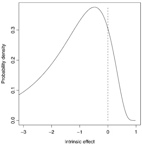
Different models lead to dramatically different trajectories of
fitness as a function of mutational step over an adaptive walk (Figure 3A). When mutations affectr, the trajectories for the additive, multiplicative, and stickbreaking models are approximately linear, exponential, and rapidly decelerating, respectively. When mutations instead affect l, the trajecto-ries are shifted: additive becomes modestly decelerating, multiplicative becomes approximately linear, and decelera-tion under stickbreaking becomes very slightly exaggerated. Note that the theoretical expectations from Table 1 (Figure 3A, shaded lines) are qualitatively correct; the disparities between them and the simulations (Figure 3A, solid lines) reflect the limited pool of beneficial mutations and the bi-ased nature in which selectionfixes mutations.
A survey of the experimental evolution literature indi-cates that, in most cases, the observed fitness trajectory decelerates as adaptation proceeds. This result has been observed inEscherichia coli(Lenski and Travisano 1994; de Visseret al.1999; Barricket al.2009), the DNA bacterioph-agesuX174 and G4 (Bullet al.1997; Wichmanet al.1999; Holder and Bull 2001), RNA bacteriophage (Burch and Chao 1999; Betancourt 2009), and the animal RNA virus, vesicular stomatitis virus (VSV) (Elena et al. 1998). The exceptions we are aware of are approximately linear trajec-tories inSaccharomyces cerevisiae(Desaiet al.2007) and in one study on VSV (Novellaet al.1995). Of the models con-sidered here, both stickbreaking models show rapidly decel-erating trajectories and the additive model on l shows a moderately decelerating trajectory.
This suggests that one of these three models is likely nearer the truth than the model most commonly assumed in
the literature, additivity on r (multiplicative onl) with its approximately linear trajectory. There are at least two reasons to be somewhat cautious regarding this conclusion. First, our results are based on SSWM dynamics while many experimen-tal and real world systems involve interference dynamics with more than one mutation contending simultaneously. Under interference dynamics, selection is more efficient at fixing bigger-effect mutations early in a walk compared to SSWM conditions (Rozen et al.2002; Barrett et al.2006). We can obtain a bound on this effect by assuming the pool of con-tending mutations is the entire pool of beneficial mutations and selection thereforefixes them in descending order from the largest to the smallest. Figure 3B shows this trajectory. As expected, interference shifts all the trajectories toward a de-celerating pattern although the effect is modest.
Second, trajectories are affected by whether fitness is considered a function of mutational step (as we have done thus far) or time. Plottingfitness against time instead of step bends most of the trajectories toward a more concave, decelerating shape (Figure 3C). Under all models, there is a tendency tofix mutations from larger to smaller intrinsic effect. When all else is equal, this leads to selection coeffi -cients (as traditionally defined, see Simulations) tending
from large to small and, therefore, to waiting times between
fixation events tending from short to long. In the“add onr” model, this is the only effect, and the trajectory decelerates moderately. In the“add onl”model there is also the effect that as fitness grows in an additive way, the proportional effect of each added mutation (the selection coefficient) becomes smaller. The stickbreaking models are most dra-matically affected by the timescale because as they approach their boundary, selection coefficients become very small and
waiting times very long. At the other extreme lies the“mult onr”model where selection coefficients actually get larger as the walk proceeds, causing the walk to accelerate in time for most of its duration. We leave a statistical treatment of trajectory data for later work and here emphasize three things: (i) most of the models show decelerating trajecto-ries, (ii) the slowdown is exaggerated both by clonal inter-ference and by using time rather than step as the explanatory variable, and (iii) with or without these infl u-ences, the stickbreaking models show much more dramatic decelerating effects than the other models.
Distribution offitness over replicate walks
When mutations affect Malthusian fitness, r, and fitness is measured as r, the theoretical distributions from replicate walks (Appendix) are log normal, normal, and negative log normal for the additive, multiplicative, and stickbreaking models (solid lines in Figure 4, A–C). When mutations affect linstead, these qualitative patterns are only slightly changed with heavier left tails (Figure 4, D and E). These predictions are based on asymptotic assumptions that (i) the total num-ber of beneficial mutations,M, is large, (ii) the step where
fitness is measured is far smaller than the number of
beneficial mutations,m>M, and (iii)mis large enough for the law of large numbers to apply. In reality,Mwill often be modest (e.g., 10,M,100) andmmay be relatively small (e.g.,#30). The simulations shed light on what effect vio-lating these assumptions has.
Early in a walk (m# 10) there is good agreement be-tween the observed and predicted distributions (Figure 4) in terms of both mean and variance. As a walk approaches its midpoint, observed means are notably smaller than the pre-dicted means because the theory assumes constant effect sizes while, in simulated walks, fitness increase slows as large-effect mutations are removed from the available pool. Still, the shapes of the distributions remain the same even when m is large. The different models make qualitatively different predictions about the distribution offitness during replicate adaptive walks: both stickbreaking models predict heavy left tails, the multiplicative onrmodel a heavy right tail, and both additive models an approximately normal distribution. Whether mutations affectrandl is relatively minor. Note also that the distributions are in terms of num-ber of mutationsfixed (steps), not time elapsed. As shown in theFitness trajectory subsection above, different modelsfix mutations in different lengths of time (Figure 3C) and will therefore achieve the distributions shown in Figure 4 at different rates (see theAppendixfor details).
Epistasis
Epistasis occurs when the fitness effect of a mutation depends on the genetic background. We investigate epistasis in two ways: first as the effect of a single mutation across
a procession of backgrounds and second as departures from additivity when a set of single mutations is combined. For the first approach, we simulate replicate walks of 10 mutational steps under each model on a single landscape. We then imagine taking the mutation that fixed 10th and engineering it into each of the preceding backgrounds in the walk. (Our choice of the 10th mutation is arbitrary, but using other stop points does not change the qualitative patterns observed; data not shown).
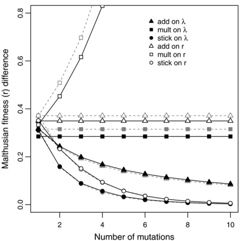
The solid lines in Figure 5 show the means of simulation results when fitness effects are defined as differences inr while the shaded lines give the theoretical relationships (Ta-ble 2). The results show how the observed fitness effects change along the walk under the different models for the same mutation (or as the intrinsic effect is held constant). Effect sizes grow exponentially for the mult onrmodel, are constant for the add onr(mult onl) model, decay moder-ately for add onl, and show rapidly diminishing effects for both stickbreaking models. Of course, these patterns closely reflect the previously discussedfitness trajectories. Here we are considering how the vertical distance (fitness) between steps qualitatively changes along a walk when the intrinsic effect is held constant. It is also noteworthy that because differences in rare, in fact, selection coefficients, Figure 5 illustrates how selection coefficients change across a walk under each model. As discussed above, this, in turn, explains how waiting times between mutations change across a walk (Figure 3C).
In the literature, epistasis is more commonly quantified as the departure from additivity when single mutations are combined. We again simulated replicate walks under each model on a single landscape. For thefirstmmutations that
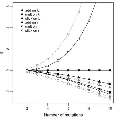
fixed, we imagined engineering each into the wild type and measuring theirfitness effects (as difference inr). In keep-ing with the literature, we predicted fitness on the basis of the additivity of the rmodel (i.e., summingfitness effects). Epistasis is then defined as e¼ robs2 rpred. For beneficial mutations e , 0 and e . 0 are termed antagonistic and synergistic epistasis, respectively.
The patterns ofe(Figure 6) are similar to those observed in Figure 5. The stickbreaking models show strong antago-nistic epistasis, add onlshows moderate antagonistic epis-tasis, add on l (mult on r) shows no epistasis (by definition), and mult onrshows strong synergistic epistasis. In fact, it is easy to understand whye(Figure 6) andfitness effect (Figure 5) must follow the same basic pattern. Con-sider two mutations,A1andA2. Ife,0 (antagonistic epis-tasis), thenrobs,rpred. LettingDrdenotefitness effect onr andrwtdenote the wild-typefitness, this implies thatrwt+ Dr1|wt + Dr2|1 , rwt + Dr1|wt + Dr2|wt, which implies Dr2|1,Dr2|wt, or a diminishing effect. Similar arguments can be made fore¼0 ande.0.
In the experimental evolution literature, the commonly observed patterns of epistasis are (1) diminishing effects, where the same mutation has smaller effects on more fit backgrounds and conversely larger effects on less fit ones,
and (2) antagonistic epistasis is more frequent than syner-gistic epistasis (Burchet al.2003; Sanjuán and Elena 2006). For example, Bullet al.(2000) found that thefitness effect of one mutation (1727T) in the bacteriophageuX174 decreased across four backgrounds of increasingfitness. Recently, Chou et al. (2011), Khan et al. (2011), and Kvitek and Sherlock (2011) all showed a general pattern of diminishing returns epistasis when beneficial mutations were inserted into closely related backgrounds. Similar results are found in double-mu-tant studies. Trindadeet al.(2009) found that when antibiotic resistance mutations in E. coli are combined, 42% of those showing significant epistasis are antagonistic, while only 15% show synergistic epistasis. Rokytaet al.(2011) inserted nine beneficial single mutations in a G4-like bacteriophage to form 18 double mutants and found antagonistic epistasis for all 18. Finally, a synthesis of 21 studies by Sanjuán and Elena (2006) indicated that antagonistic epistasis is more prevalent in viruses and prokaryotes, while synergistic or no epistasis is more common in eukaryotes. Thus studies have tended to show patterns of epistasis broadly consistent with the two stickbreaking models and additivity onl.
It is important to clarify that the values ofeand hence the patterns of antagonisticvs.synergistic epistasis depend on the null model used to calculate predictedfitness. It is easy to see what the patterns would be under other nulls by noting that the “predicted”and observed labels in Figure 6 are arbitrary. Figure 6 can also be thought of as showing the fitness divergence between different models as mutations of the same intrinsic effect are introduced. For any null and alternative model, the distance between them corresponds to the values ofe.
Conclusion
The stickbreaking model is based on the simple idea that mutational fitness effects should diminish the nearer the background is to the maximum fitness boundary. It solves the bookkeeping problem while also producing patterns of
fitness trajectory and epistasis broadly consistent with experimentalfindings. The next important step is to develop statistical methods for fitting and testing the stickbreaking model on real data. Like the additive and multiplicative models, stickbreaking is too simple to be biologically correct. Rather, our hope is that stickbreaking is mathematically tractable like those models, but also captures a basic bi-ological property and provides an explanatory power that those models seem to miss.
Literature Cited
Barrett, R. D. H., L. K. M’Gonigle, and S. P. Otto, 2006 The
dis-tribution of beneficial mutant effects under strong selection.
Genetics 174: 2071–2079.
Barrick, J. E., D. S. Yu, S. H. Yoon, H. Jeong, T. K. Oh et al.,
2009 Genome evolution and adaptation in a long-term
exper-iment with Escherichia coli. Nature 461: 1243–1247.
Betancourt, A. J., 2009 Genomewide patterns of substitution in
adaptively evolving populations of the RNA bacteriophage MS2.
Genetics 181: 1535–1544.
Bonhoeffer, S., C. Chappey, N. T. Parkin, J. M. Whitcomb, and C. J.
Petropoulos, 2004 Evidence for positive epistasis in HIV-1.
Sci-ence 306: 1547–1550.
Bull, J. J., M. R. Badgett, H. A. Wichman, J. P. Huelsenbeck, D. M.
Hilliset al., 1997 Exceptional convergent evolution in a virus.
Genetics 147: 1497–1507.
Bull, J. J., M. R. Badgett, and H. A. Wichman, 2000 Big-benefit
mutations in a bacteriophage inhibited with heat. Mol. Biol.
Evol. 17: 942–950.
Burch, C. L., and L. Chao, 1999 Evolution by small steps and
rugged landscapes in the RNA virusu6. Genetics 151: 921–927.
Burch, C. L., P. E. Turner, and K. A. Hanley, 2003 Patterns of
epistasis in RNA viruses: a review of the evidence from vaccine
design. J. Evol. Biol. 16: 1223–1235.
Chevin, L., 2010 On measuring selection in experimental
evolu-tion. Biol. Lett. 7: 210–213.
Chou, H., H. Chiu, N. Delaney, D. Segrè, and C. Marx,
2011 Diminishing returns epistasis among beneficial
muta-tions decelerates adaptation. Science 332: 1190–1192.
Cooper, V. S., and R. E. Lenski, 2000 The population genetics of
ecological specialization in evolvingEscherichia colipopulations.
Nature 407: 736–739.
Cowperthwaite, M. C., J. J. Bull, and L. Ancel Myers,
2005 Distributions of beneficialfitness effects in RNA.
Genet-ics 170: 1449–1457.
Desai, M. M., D. S. Fisher, and A. W. Murray, 2007 The speed of
evolution and maintenance of variation in asexual populations.
Curr. Biol. 17: 385–394.
de Visser, J. A. G. M., C. W. Zeyl, P. J. Gerrish, J. L. Blanchard, and
R. E. Lenski, 1999 Diminishing returns from mutation supply
rate in asexual populations. Science 283: 404–406.
Donnelly, P., and P. Joyce, 1989 Continuity and weak
conver-gence of ranked and size-biased permutations on an infinite
simplex. Stoch. Proc. Appl. 31: 89–103.
Elena, S. F., and R. E. Lenski, 1997 Test of synergistic interactions
among deleterious mutations in bacteria. Nature 390: 395–398.
Elena, S. F., M. Davila, I. S. Novella, J. J. Holland, E. Domingoet al.,
1998 Evolutionary dynamics offitness recovery from the
de-bilitating effects of Muller’s ratchet. Evolution 52: 309–314.
Eyre-Walker, A., and P. D. Keightley, 2007 The distribution of
fitness effects of new mutations. Nat. Rev. Genet. 8: 610–618.
Gerrish, P. J., and R. E. Lenski, 1998 The fate of competing beneficial
mutations in an asexual population. Genetica 102/103: 127–144.
Gillespie, J. H., 1991 The Causes of Molecular Evolution. Oxford
University Press, New York.
Hartl, D. L., and A. G. Clark, 1997 Principles of Population
Genet-ics, Ed. 3. Sinauer Associates, Sunderland, MA.
Holder, K., and J. Bull, 2001 Profiles of adaptation in two similar
viruses. Genetics 159: 1393–1404.
Joyce, P., D. R. Rokyta, C. J. Beisel, and H. A. Orr, 2008 A general
extreme value theory model for the adaptation of DNA sequen-ces under strong selection and weak mutation. Genetics 180:
1627–1643.
Kacser, H., and J. Burns, 1981 The molecular basis of dominance.
Genetics 97: 639–666.
Kauffman, S. A., 1993 The Origins of Order. Oxford University
Press, New York.
Khan, A., D. Dinh, D. Schneider, R. Lenski, and T. Cooper,
2011 Negative epistasis between beneficial mutations in an
evolving bacterial population. Science 332: 1193–1196.
Kim, Y., and H. A. Orr, 2005 Adaptation in sexualsvs.asexuals:
clonal interference and the Fisher–Muller model. Genetics 171:
1377–1386.
Kimura, M., 1962 On the probability offixation of mutant genes
in a population. Genetics 47: 713–719.
Kryazhimskiy, S., G. Tkacˇik, and J. Plotkin, 2009 The dynamics of
adaptation on correlated fitness landscapes. Proc. Natl. Acad.
Sci. USA 106: 18638–18643.
Kvitek, D., and G. Sherlock, 2011 Reciprocal sign epistasis
be-tween frequently experimentally evolved adaptive mutations
causes a ruggedfitness landscape. PLoS Genet. 7: e1002056.
Lenski, R. E., and M. Travisano, 1994 Dynamics of adaptation and
diversification: a 10,000-generation experiment with bacterial
populations. Proc. Natl. Acad. Sci. USA 91: 6808–6814.
MacArthur, R., 1957 On the relative abundance of bird species.
Proc. Natl. Acad. Sci. USA 43: 293–295.
Miller, C., P. Joyce, and H. Wichman, 2011 Mutational effects and
population dynamics during viral adaptation challenge current
models. Genetics 187: 185–202.
Novella, I. S., E. A. Duarte, S. F. Elena, A. Moya, E. Domingoet al.,
1995 Exponential increases of RNA virusfitness during large
pop-ulation transmissions. Proc. Natl. Acad. Sci. USA 92: 5841–5844.
Orr, H. A., 2002 The population genetics of adaptation: the
adap-tation of DNA sequences. Evolution 56: 1317–1330.
Orr, H. A., 2003 The distribution offitness effects among benefi
-cial mutations. Genetics 163: 1519–1526.
Patil, C., and C. Taillie, 1977 Diversity as a concept and its
implica-tions for random communities. Bull. Int. Stat. Inst. 47: 497–515.
R Development Core Team, 2009 R: A Language and Environment
for Statistical Computing. R Foundation for Statistical
Comput-ing, Vienna.
Rokyta, D. R., C. J. Beisel, P. Joyce, M. T. Ferris, C. L. Burchet al.,
2008 Beneficialfitness effects are not exponential for two
vi-ruses. J. Mol. Evol. 67: 368–376.
Rokyta, D. R., Z. Abdo, and H. A. Wichman, 2009 The genetics of
adaptation for eight microvirid bacteriophages. J. Mol. Evol. 69:
229–239.
Rokyta, D., P. Joyce, S. Caudle, C. Miller, C. Beisel et al.,
2011 Epistasis between beneficial mutations and the
phenotype-to-fitness map for a ssdna virus. PLoS Genet. 7: e1002075.
Rozen, D. E., J. A. G. M. de Visser, and P. J. Gerrish, 2002 Fitness
effects of fixed beneficial mutations in microbial populations.
Curr. Biol. 12: 1040–1045.
Sanjuán, R., and S. F. Elena, 2006 Epistasis correlates to genomic
complexity. Proc. Natl. Acad. Sci. USA 103: 14402–14405.
Sanjuán, R., A. Moya, and S. F. Elena, 2004 The distribution of
fitness effects caused by single-nucleotide substitutions in an
RNA virus. Proc. Natl. Acad. Sci. USA 101: 8396–8401.
Schoustra, S. E., T. Bataillon, D. R. Gifford, and R. Kassen,
2009 The properties of adaptive walks in evolving populations
of fungus. PLoS Biol. 7: e1000250.
Silander, O. K., O. Tenaillon, and L. Chao, 2007 Understanding
the evolutionary fate offinite populations: the dymanics of
mu-tational effects. PLoS Biol. 5: e94.
Trindade, S., A. Sousa, K. Xavier, F. Dionisio, M. Ferreira et al.,
2009 Positive epistasis drives the acquisition of multidrug
re-sistance. PLoS Genet. 5: e1000578.
Weinreich, D. M., N. F. Delaney, M. A. DePristo, and D. L. Hartl,
2006 Darwinian evolution can follow only very few
muta-tional paths tofitter proteins. Science 312: 111–114.
Wichman, H. A., M. R. Badgett, L. A. Scott, C. M. Boulianne, and J.
J. Bull, 1999 Different trajectories of parallel evolution during
viral adaptation. Science 285: 422–424.
Wichman, H. A., J. Millstein, and J. J. Bull, 2005 Adaptive
molec-ular evolution for 13,000 phage generations: a possible arms
race. Genetics 170: 19–31.
Woods, R., D. Schneider, C. Winkworth, M. Riley, and R. Lenski,
2006 Tests of parallel molecular evolution in a long-term
ex-periment withEscherichia coli. Proc. Natl. Acad. Sci. USA 103:
9107–9112.
Appendix
Distribution of Total Fitness Effects AftermSteps of Adaptation
We show here that there are three limiting distributions for thefitness achieved aftermsteps in a walk: the normal dis-tribution under additivity, the log normal under the multipli-cative model, and negative log normal under stickbreaking.
Denote the“intrinsic”fitness effect of the beneficial mu-tation Ai by xi. For the additive model xi = Dwi, for the multiplicative modelxi=si, and for the stickbreaking model xi=ui. Note that uiandsi are just different ways to scale Dwi. That is, ui = Dwi/(d 2 wwt) and si = Dwi/wwt. Therefore
uj PM
i¼1 ui
¼ Dwj=ðd2wwtÞ
PM
i¼1 Dwi=ðd2wwtÞ
¼ Dwj
PM i¼1 Dwi
and similarly sj PM
i¼1 si¼
Dwj=wwt
PM
i¼1 Dwi=wwt¼
Dwj PM
i¼1 Dwi:
Throughout we assume that the walks evolve according to SSWM conditions. We also assume that for each value ofM, x1, x2,. . .,xM is fixed. That is, we use the same set of in-trinsicfitness effects for replicate walks.
Consider an adaptive walk of lengthm. LetYibe the in-trinsic fitness effect of the mutation arising at step i. The joint distribution ofY1,Y2,. . .,Ymcan be described as
PY1¼xi1;Y2¼xi2; :::;Ym¼xim
¼Pxi1
M i¼1 xi
xi2 PM
i6¼i1 xi xi3 PM
i6¼i1;i2 xi
⋯P xim
M
i6¼i1;:::;im21 xi
:
(A1) Note that Y1, Y2,. . .,Ym are dependent random variables. The dependence comes from the fact that once a mutation is used in a walk it will not be used again, thus reducing the number of available mutations at each step. However, ifMis large enough, we show below thatY1,Y2,. . .,Ymare approx-imately independent and identically distributed. Let x(1)= max{x1,x2,. . .,xM}. Note thatxi1þ: : :þxim21#ðm21Þxð1Þ. Therefore,
x$ 1
M XM
i6¼i1;:::;im21
xi$x2
ðm21Þxð1Þ
M : (A2)
Here is where the relationship betweenMand mbecomes important. We assume that m is an order of magnitude smaller thanM. More precisely, we assume that asM/N, thenmln(M)/M/0 andm/N. It follows from extreme value theory that for large M,x(1)c lnM. [More precisely x(1)/ln(M) converges to a constantcasM/N.] Taking the limit as M / N in inequality (A2) reveals that limM/Nx2ð1= MÞPMi6¼i1;:::;im21xi¼0: Thus for large M,
ð1= MÞPMi6¼i1;:::;ik21xix, for k = 1, 2,. . .,m. If we replace the denominators in Equation A1 with M x, then this leads to the assumption that Y1, Y2,. . .,Ym are approximately in-dependent and identically distributed with PðY¼xÞ x= M x: Note that EðYÞ ¼ ðPMi¼1 x2i=MÞ=x and VarðYÞ ¼ ðPMi¼1 x3i=MÞ=x2ðð
PM
i¼1x2i=MÞ=xÞ 2
. Both converge asM/N.
Normal, Log Normal, and Negative Log Normal
Below we review the three central distributions associated withmsteps of an adaptive walk. Thenormal distributionis given by
fX
xm;s2¼ ffiffiffiffiffiffi1 2p
p
se2ð
1=2Þððx2mÞ=sÞ2: (A3)
If X follows the normal distribution, we say that V = eX follows the log-normal distributionwith probability density function given by
fV
vm;s2 ffiffiffiffiffiffi1 2p
p
sve2ð
lnðvÞ2mÞ2=ð2s2Þ
; (A4)
and if V follows the log normal, we say that W = 1 2 V follows thenegative log-normal distributionwith probability density function given by
fWðwÞ ¼ ffiffiffiffiffiffi 1 2p
p
sð12wÞe
2ðlnð12wÞ2mÞ2=ð2s2Þ
: (A5)
Note that the parametersmandsappear in all three prob-ability densities, but must be interpreted differently in each. Whilemrepresents the mean ands2represents the variance of a normal, the mean of the log-normal distribution is EðVÞ ¼EðeXÞ ¼emþs2=2
and the variance of a log normal is VarðVÞ ¼Eðe2X2ðEeXÞ2¼
e2mþs2ðes221Þ. If W is negative log normal, then the mean isEðWÞ ¼12EðVÞ ¼12emþs2=2 and the variance of a negative log normal is the same as that of a log normal.
Now ifYirepresents thefitness differences, then thefi t-ness aftermsteps is given byw1;2;:::;m¼wwtþ
Pm
i¼1Yi: Un-der the additive model, the central limit theorem applies and the distribution ofw1,2,. . .,mwill be approximately normal with meanm¼wwtþmEðYÞ ¼wwtþmððPiM¼1x2i= MÞ=xÞand s2¼m VarðYÞ¼mððPM
i¼1 x3i=MÞ=xÞ2mððð PM
i¼1 x2i=MÞ=xÞÞ 2
. However, if the multiplicative model applies, thenw1;2;:::; m¼ wwtQmi¼1ð1þYiÞ. This implies w1;2;:::;m=wwt¼e
Pm i¼1lnð1þYiÞ: The central limit theorem now applies to Pmi¼1lnð1þYiÞ: Thusm¼mEðlnð1þYÞÞ ¼mPMj¼1xjlnð1þxjÞ=ðN xÞand
s2¼m Varðlnð1þYÞÞ
¼mX
M
j¼1
ln1þxj 2
xj
ðN xÞ 2
PM j¼1xjln
1þxj
ðN xÞ
!2! :
Under the stickbreaking model, ðwi;1;:::; m2wwtÞ=d¼
12Qm
i¼1ð12YiÞis approximately negative log normal, where m=mE(12Y) ands2=mVar(12Y) and the formulas are analogous to those of the log normal.
The assumption that Mis large enough so thatmis an order of magnitude smaller yetmis still large enough for the central limit theorem to apply is not always going to be achieved. Simulations can help in determining the degree to which violation of assumptions matters.
Number of Stepsvs.Time to Adaptation
Under SSWM conditions the time it takes a mutation with selection coefficient s to arise and fix in the population is exponentially distributed with mean 1/Nms, wheremis the beneficial mutation rate andNis the population size. Now if there are a total of M beneficial mutations available, the time in generations to fixation of thefirst beneficial muta-tion is on average 1=ðNmMsÞ;wheresis the average
selec-tion coefficient among theMavailable mutations. All of our theory is based on the asymptotic results formed by taking the limit asMgoes to infinity. AsMgoes to infinity the time to fixation converges to zero. So a timescale change is re-quired. If we assume that 1 unit of time is equivalent toNmM generations, then the mean time for thefirst beneficial mu-tation to fix using this timescale will be exponentially dis-tributed with mean 1=s. In the limit asMgoes to infinity,s converges to the mean of the distribution of beneficial muta-tions, which we denote byg. We now use an extension of the central limit theorem that states PMti¼1ððYi2mmÞ=
ffiffiffiffiffiffi Mt
p
sÞ
converges to the normal distribution ast/N. This shows that the time limit prediction of the additive model is nor-mal. Applying the analogous central limit theorem result to PMt
i¼1lnð1þYiÞ shows that the multiplicative model leads to a log-normal distribution. Applying the analogous cen-tral limit theorem result to PMt