ISSN (Print) : 2347 - 6710
I
nternationalJ
ournal ofI
nnovativeR
esearch inS
cience,E
ngineering andT
echnologyVolume 3, Special Issue 3, March 2014
2014 International Conference on Innovations in Engineering and Technology (ICIET’14) On 21st & 22nd March Organized by
K.L.N. College of Engineering, Madurai, Tamil Nadu, India
Voltage Stability Margin Assessment Using
Neural Network
Dr.K.Gnanambal, K.R.Jeyavelmani
Department of Electrical & Electronics Engineering, K.L.N. College of Engineering, Pottapalayam, India.
Department of Electrical & Electronics Engineering, K.L.N. College of Engineering, Pottapalayam, India.
ABSTRACT— As power systems become more complex and heavily loaded, voltage stability becomes an increasing serious problem. Voltage instability problem increases day by day because of the increase in demand. It is necessary to analyze the power system with respect to voltage stability. At present, solar energy is increasingly penetrating into electrical grids. It is necessary to analyze the system stability with the inclusion of PV panel. Several methods are found in the literature for the modeling of PV panel. In this work, I am going to adapt a suitable model of the photovoltaic cell. The model should be able to relate the inputs such as irradiance and temperature with the output voltage and power that can be generated by the PV panel. The PV model will be included at any one of the existing buses and the system stability will be analyzed using PSAT software. In many literatures, the voltage stability of the grid with PV panel is analyzed but they consider the PV panel as a constant power source. But it is not practically so, hence in this paper I am going to adapt a suitable PV model and hence the stability limit i.e. the maximum load ability limit of the system is obtained for various irradiance and temperature levels. The voltage stability will also be analyzed under various contingencies.
KEYWORDS— Neural Network (NN), Photovoltaic Panel (PV panel), Maximum Load ability Limit, Voltage Stability
I. INTRODUCTION
Power system stability is defined as a characteristic for a power system to remain in a state of equilibrium at normal operating conditions and to restore an acceptable state of equilibrium after a disturbance. The stability problem has been the rotor angle stability, i.e. maintaining synchronous operation. Instability may also occur without loss of synchronism, in which case the concern is the control and stability of voltage. The voltage stability is defined as follows:
“The voltage stability is the ability of power system to maintain steady acceptable voltages at all buses in the system at normal operating conditions and after being subjected to a disturbance”.
Voltage stability is a fundamental component of dynamic security assessment and it has been emerged as a major concern for power system security and a main limit for loading and power transfer. Voltage Stability is a problem in power systems, which are heavily loaded, faulted or have a shortage of reactive power. The problem of voltage stability concerns the whole power system, although it usually has a large involvement in one critical area of power system.
Fig.1 Curves Representing Voltage Security
difficulty. Power System Analysis Toolbox (PSAT) in tracing the PV curve for obtaining Maximum Loading Point (Pmax) involves the input from PV modeling with 6-bus benchmark system. By varying the real power generation the maximum load ability limit points are obtained.
II. GENERAL INTRODUCTION ABOUT POWER
SYSTEM ANALYSIS TOOLBOX (PSAT)
PSAT has been thought to be portable and open source. At this aim, PSAT has been developed using MATLAB, which runs on the commonest operating systems, such as Unix, Linux, Windows and Mac OS X. Nevertheless, PSAT would not be completely open source if it run only on MATLAB, which is a proprietary software. At this aim PSAT can run also on the latest GNU / Octave releases, which is basically a free MATLAB clone. In the knowledge of the author, PSAT is actually the first free software project in the field of power system analysis. PSAT is also the first power system software which runs on GNU / Octave platforms.
Once the power flow has been solved, the user can perform further static and / or dynamic analyses. These are:
1. Continuation Power Flow (CPF). 2. Optimal Power Flow (OPF). 3. Small signal stability analysis. 4. Time domain simulations.
PSAT deeply exploits Matlab vectorized computations and sparse matrix functions in order to optimize performances. Furthermore PSAT is provided with the most complete set of algorithms for static and dynamic analyses among currently available Matlab-based power system software’s (see Table 5.1). PSAT also contains interfaces to UWPFLOW and GAMS which highly extend PSAT ability to solve CPF and OPF problems, respectively. These interfaces are not discussed here, as they are beyond the main purpose of this paper.
In order to perform accurate and complete power system analyses, PSAT supports a variety of static and dynamic models, as follows:
Power Flow Data: Bus bars, transmission lines and transformers, slack buses, PV generators, constant power loads, and shunt admittances.
Market Data: Power supply bids and limits, generator power reserves, and power demand bids and limits.
Switches: Transmission line faults and breakers.
Measurements: Bus frequency measurements. Loads: Voltage dependent loads, frequency dependent loads, ZIP (polynomial) loads,
thermostatically controlled loads, and exponential recovery loads.
Machines: Synchronous machines (dynamic order from 2 to 8) and induction motors (dynamic order from 1 to 5)
Controls: Turbine Governors, AVRs, PSSs, Over-excitation limiters, and secondary voltage regulation.
Regulating Transformers: Under load tap changers and phase shifting transformers. FACTS: SVCs, TCSCs, SSSCs, UPFCs. Wind Turbines: Wind models, constant speed
wind turbine with squirrel cage induction motor, variable speed wind turbine with doubly fed induction generator, and variable speed wind turbine with direct drive synchronous generator.
Other Models: Synchronous machine dynamic shaft, sub-synchronous resonance model, solid oxide fuel cell, and sub-transmission area equivalents.
Fig.2. Main graphical user interface of PSAT
III. CONTINUATION POWER FLOW
Continuation power flow is one method to determine the proximity to voltage collapse point and can be described as a power flow solution, which is used to analyze the stability of power system under normal and disturbance conditions. The main purpose of Continuation Power Flow is to find a continuity of power flow solution for a given load change. Conventional power flow algorithms are subjected to the convergence problems at operating condition near the stability limit. Therefore researchers proposed to use the Continuation Power Flow to solve this problem by reformulating the power flow equations and ensuring the system remains in well-conditioned at all possible loading condition. This Continuation Power Flow uses an iterative process involving predictor and corrector step.
IV. COMPUTATION OF MAXIMUM LOADING
POINT
point can be calculated by starting at the current operating point, making small increments in loading and production and re-computing load-flows at each increment until the maximum point is reached. The load-flow diverges close to maximum loading point because there are numerical problems in the solutions of load-flow equations. The load-flow based method is not the most efficient, but has the following characteristics making it appropriate for voltage stability studies:
Good models for the equipment operating limits: generator capability limits, transformer tap ranges, circuit ratings and bus voltage criteria.
Good models for the discrete controls: transformer taps steps and switched shunts. Capability to recognize the maximum loading
points though the minimum singular value of load-flow Jacobin matrix.
Familiar computer modeling, data requirements and solutions algorithms. Option of using the existing computer
programs with minor modifications.
V. ARTIFICIAL NEURAL NETWORK
An Artificial Neural Network (ANN) is an efficient information processing system which resembles in characteristics with a biological neural network. ANNs posses large number highly interconnected processing elements called nodes or units or neurons, which usually operate in parallel and are configured in regular architectures. Each neuron is connected with the other by a connection link. Each connection link is associated with weights which contain information about the input signal. This information is used by the neuron net to solve a particular problem. ANN’s collective behavior is characterized by their ability to learn, recall and generalize training patterns or data similar to that of a human brain. They have the capability to model networks of original neurons as found in the brain. Thus, the ANN processing elements are called neurons or artificial neurons.
Neural networks, with their remarkable ability to derive meaning from complicated or imprecise data, can be used to extract patterns and detect trends that are too complex to be noticed by either humans or other computer techniques. A trained neural network can be thought of as an “expert” in the category of information it has been given to analyze. This expert can then be used to provide projections given new situations of interest and answer “what if” questions.
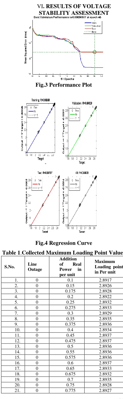
VI. RESULTS OF VOLTAGE
STABILITY ASSESSMENT
Fig.3 Performance Plot
Fig.4 Regression Curve
Table 1.Collected Maximum Loading Point Values
S.No. Line
Outage
Addition
of Real
Power in
per unit
Maximum Loading point in Per unit
1. 0 0.1 2.8917
2. 0 0.15 2.8926
3. 0 0.175 2.8928
4. 0 0.2 2.8922
5. 0 0.25 2.8932
6. 0 0.275 2.8933
7. 0 0.3 2.8929
8. 0 0.35 2.8935
9. 0 0.375 2.8936
10. 0 0.4 2.8934
11. 0 0.45 2.8937
12. 0 0.475 2.8937
13. 0 0.5 2.8936
14. 0 0.55 2.8936
15. 0 0.575 2.8936
16. 0 0.6 2.8937
17. 0 0.65 2.8933
18. 0 0.675 2.8932
19. 0 0.7 2.8935
20. 0 0.75 2.8928
22. 1 0.1 2.8869
23. 1 0.15 2.8873
24. 1 0.175 2.8884
25. 1 0.2 2.8891
26. 1 0.25 2.8907
27. 1 0.275 2.8919
28. 1 0.3 2.8927
29. 1 0.35 2.8937
30. 1 0.375 2.894
31. 1 0.4 2.8942
32. 1 0.45 2.8946
33. 1 0.475 2.8947
34. 1 0.5 2.8948
35. 1 0.55 2.8949
36. 1 0.575 2.8949
37. 1 0.6 2.895
38. 1 0.65 2.8933
39. 1 0.675 2.8932
40. 1 0.7 2.8949
41. 1 0.75 2.8948
42. 1 0.775 2.8946
43. 2 0.1 2.8307
44. 2 0.15 2.8343
45. 2 0.175 2.836
46. 2 0.2 2.8371
47. 2 0.25 2.8403
48. 2 0.275 2.8416
49. 2 0.3 2.8432
50. 2 0.35 2.8455
51. 2 0.375 2.8467
52. 2 0.4 2.8482
53. 2 0.45 2.8505
54. 2 0.475 2.8517
55. 2 0.5 2.8526
56. 2 0.55 2.8547
57. 2 0.575 2.8558
58. 2 0.6 2.8563
59. 2 0.65 2.8584
60. 2 0.675 2.8593
61. 2 0.7 2.8601
62. 2 0.75 2.8613
63. 2 0.775 2.8622
64. 3 0.1 2.6647
65. 3 0.15 2.6651
66. 3 0.175 2.6652
67. 3 0.2 2.6653
68. 3 0.25 2.6655
69. 3 0.275 2.6655
70. 3 0.3 2.6656
71. 3 0.35 2.6656
72. 3 0.375 2.6657
73. 3 0.4 2.6657
74. 3 0.45 2.6659
75. 3 0.475 2.6659
76. 3 0.5 2.6659
77. 3 0.55 2.6659
78. 3 0.575 2.6659
79. 3 0.6 2.6658
80. 3 0.65 2.6657
81. 3 0.675 2.6657
82. 3 0.7 2.6657
83. 3 0.75 2.6656
84. 3 0.775 2.6655
85. 4 0.1 2.1256
86. 4 0.15 2.1256
87. 4 0.175 2.1256
88. 4 0.2 2.1256
89. 4 0.25 2.1255
90. 4 0.275 2.1255
91. 4 0.3 2.1255
92. 4 0.35 2.1253
93. 4 0.375 2.1253
94. 4 0.4 2.1252
95. 4 0.45 2.1249
96. 4 0.475 2.1248
97. 4 0.5 2.1247
98. 4 0.55 2.1243
99. 4 0.575 2.1242
100. 4 0.6 2.1224
101. 4 0.65 2.1235
102. 4 0.675 2.1232
103. 4 0.7 2.123
104. 4 0.75 2.1223
105. 4 0.775 2.1221
106. 5 0.1 2.7449
107. 5 0.15 2.7445
108. 5 0.175 2.7444
109. 5 0.2 2.7442
110. 5 0.25 2.7436
111. 5 0.275 2.7436
112. 5 0.3 2.7435
113. 5 0.35 2.743
114. 5 0.375 2.7431
115. 5 0.4 2.743
116. 5 0.45 2.7426
117. 5 0.475 2.7424
118. 5 0.5 2.7422
119. 5 0.55 2.7418
120. 5 0.575 2.7415
121. 5 0.6 2.7413
122. 5 0.65 2.7407
123. 5 0.675 2.7407
124. 5 0.7 2.7401
125. 5 0.75 2.7394
126. 5 0.775 2.7393
127. 6 0.1 1.6033
128. 6 0.15 1.6032
129. 6 0.175 1.6031
130. 6 0.2 1.6031
131. 6 0.25 1.6029
132. 6 0.275 1.6028
133. 6 0.3 1.6028
134. 6 0.35 1.6026
135. 6 0.375 1.6025
136. 6 0.4 1.6024
137. 6 0.45 1.6022
138. 6 0.475 1.602
139. 6 0.5 1.6019
140. 6 0.55 1.6016
141. 6 0.575 1.6015
142. 6 0.6 1.6013
143. 6 0.65 1.6009
144. 6 0.675 1.6007
145. 6 0.7 1.6004
146. 6 0.75 1.5998
147. 6 0.775 1.5995
148. 7 0.1 2.8944
149. 7 0.15 2.8948
150. 7 0.175 2.8949
151. 7 0.2 2.895
152. 7 0.25 2.8952
153. 7 0.275 2.8953
154. 7 0.3 2.8953
155. 7 0.35 2.8954
156. 7 0.375 2.8959
157. 7 0.4 2.896
158. 7 0.45 2.8962
159. 7 0.475 2.8962
160. 7 0.5 2.8963
161. 7 0.55 2.7418
162. 7 0.575 2.7415
164. 7 0.65 2.8964
165. 7 0.675 2.8963
166. 7 0.7 2.8963
167. 7 0.75 2.8962
168. 7 0.775 2.8961
169. 8 0.1 2.3967
170. 8 0.15 2.3955
171. 8 0.175 2.3972
172. 8 0.2 2.3974
173. 8 0.25 2.3977
174. 8 0.275 2.3978
175. 8 0.3 2.3979
176. 8 0.35 2.3982
177. 8 0.375 2.3983
178. 8 0.4 2.3984
179. 8 0.45 2.3986
180. 8 0.475 2.3986
181. 8 0.5 2.3988
182. 8 0.55 2.399
183. 8 0.575 2.399
184. 8 0.6 2.3991
185. 8 0.65 2.3992
186. 8 0.675 2.3992
187. 8 0.7 2.3993
188. 8 0.75 2.3993
189. 8 0.775 2.3993
190. 9 0.1 2.1527
191. 9 0.15 2.1537
192. 9 0.175 2.1542
193. 9 0.2 2.1546
194. 9 0.25 2.1553
195. 9 0.275 2.1556
196. 9 0.3 2.1559
197. 9 0.35 2.1265
198. 9 0.375 2.1567
199. 9 0.4 2.1568
200. 9 0.45 2.1571
201. 9 0.475 2.1577
202. 9 0.5 2.158
203. 9 0.55 2.1585
204. 9 0.575 2.1578
205. 9 0.6 2.1585
206. 9 0.65 2.1592
207. 9 0.675 2.1594
208. 9 0.7 2.1596
209. 9 0.75 2.1599
210. 9 0.775 2.16
211. 10 0.1 2.8666
212. 10 0.15 2.8684
213. 10 0.175 2.8709
214. 10 0.2 2.8715
215. 10 0.25 2.8746
216. 10 0.275 2.8754
217. 10 0.3 2.8769
218. 10 0.35 2.879
219. 10 0.375 2.8794
220. 10 0.4 2.8815
221. 10 0.45 2.8831
222. 10 0.475 2.8835
223. 10 0.5 2.8844
224. 10 0.55 2.873
225. 10 0.575 2.8868
226. 10 0.6 2.8871
227. 10 0.65 2.8893
228. 10 0.675 2.8898
229. 10 0.7 2.8903
230. 10 0.75 2.891
231. 10 0.775 2.8927
VII. CONCLUSION
Power System tool box (PSAT) is used to determine the nose point of PV curve. This result is obtained using PSAT are given as the training data to Artificial Neural Network (ANN). The trained network is used to predict the maximum loading point.
Causal Productions permits the distribution and revision of these templates on the condition that Causal Productions is credited in the revised template as follows: “original version of this template was provided by courtesy of Causal Productions (www.causalproductions.com)”.
REFERENCES
[1] Weidong Xiao, Fonkwe Fongang Edwin, “Efficient Approaches for Modeling and simulating Photovoltaic Power Systems”, IEEE Journal of Photovoltaics, Vol.3, No.1, Januray 2013.
[2] Jie Shi, Wei-Jen Lee, “Forecasting Power Output of Photovoltaic Systems Based on Weather Classification and Support Vector Machines”, IEEE Transactions of Industry Applications, Vol.48, No.3, May/ June 2012. [3] Filippo,Maria Savino, “Uncertainty Analysis in
Photovoltaic Cell Parameter Estimation”, IEEE Transactions on Instrumentation and Measurement, Vol.61, No.5, May 2012.
[4] Abir Chatterjee,Ali Keyhani, “Identification of Photovoltaic Source Models”, IEEE Transactions on Energy Conversion, Vol.26, No.3, September 2011. [5] Marcelo Gradella,Jonas Rafael, “Comprehensive
Approach to Modeling and Simulation of Photovoltaic Arrays”, IEEE Transactions on Power Electronics, Vol.24, No.5, May 2009.
[6] Jan T. Bialasiewicz, “Renewable Energy Systems with Photovoltaic Power Generators: Operation and Modeling”, IEEE Transactions on Industrial Electronics, Vol.55, No.7, July 2008.
[7] W.Richard, A.Johnson, “Simulink Model for Economic Analysis and Environmental Impacts of a PV With Diesel – Battery System for Remote Villages”IEEE Transactions on Power Systems, Vol.20, No.2, May 2005.
[8] Yun Tiam Tan, Daniel S., “A Model of PV Generation Suitable for Stability Analysis”, IEEE Transactions on Energy Conversion, Vol.19, No.4, December 2004. [9] Dingguo Chan,Ronald.R., “Neural-Network- Based load
modeling and its use in voltage stability analysis”, IEEE Transactions on Control Systems Technology, Vol.11, No.11, 4th July 2003.