From Single DNA Molecules to an
Entire Virus: an Investigation with
Quantitative Fluorescence Microscopy
and X-Ray Reflectivity
Marion Hochrein
From Single DNA Molecules to an
Entire Virus: an Investigation with
Quantitative Fluorescence Microscopy
and X-Ray Reflectivity
Marion Hochrein
Dissertation
im Department f¨
ur Physik
der Ludwig–Maximilians–Universit¨
at
M¨
unchen
vorgelegt von
Marion Hochrein
aus M¨
unchen
Erstgutachter: Prof. Dr. J. O. R¨
adler
Zweitgutachter: Prof. Dr. E. Frey
Vielen Dank an ...
Prof. Dr. Joachim R¨adler f¨ur die M¨oglichkeit, diese Doktorarbeit an seinem Lehrstuhl durchzuf¨uhren, die gute Betreuung und die große experimentelle Freiheit.
Dr. Bert Nickel f¨ur die Einf¨uhrung in die Reflektivit¨at, viele tolle Experimente am Desy und an der ESRF, seine Geduld beim Erkl¨aren und die produktive Zusammenarbeit am Membranenpaper.
Prof. Leonardo Golubovic thanks for the great and longlasting cooperation and the interesting theory to the DNA stretching experiments.
Dr. Lucienne Letellier thanks for the fruitful cooperation on the T5 phage ejection project.
Dr. Stephanie Mangenot thanks for the great time we had when we were doing exper-iments in the dark microscopy room and when cooking noodles ...
Christian Reich die tolle Zeit an den Synchrotrons, viel Spaß und super Experimente. Ich w¨unsche dir weiterhin Happy Lipids!
Dr. Christine Meyer f¨ur die super scharfen REM Bilder, die kein anderer so gut hinge-bracht hat. Außerdem danke ich dir f¨ur die gemeinsamen Versuche einen idealen Master herzustellen. So habe ich einen Einblick in die Arbeitsmethoden am Halb-leiterlehrstuhl erhalten.
Dr. Heribert Lorenz f¨ur die strukturierten Siliziumwafer.
Dr. Ulf R¨adler daf¨ur, dass du unerm¨udlich die strukturierte Folie an die Ibidikammern geklebt hast. Vielen Dank auch daf¨ur, dass du mir in der schweren Anfangsphase oft zur Hand gegangen bist.
Andreas Hohner f¨ur seine nette hilfsbereite Art. Es hat Spaß gemacht, mit dir Praktika zu ¨uberleben und das B¨uro zu teilen. Auf dich kann man sich verlassen. Vor allem wenn Igor h¨angt.
Dr. Simon Keller die unz¨ahligen K¨asten Bier, die unvergeßliche Rossler-Erfahrung und die Einblicke ins isometrische Freeciv.
Stefan Beyer weil du mir den Einstieg erleichtert hast, indem wir zusammen an un-m¨oglichen Experimenten herumversuchen konnten. Auch vielen Dank f¨ur die AFM Messungen im Reinraum.
Dr. Valentin Kahl f¨ur die Einf¨uhrung in das DNA auf Lipid System. Judith Leierseder die beste Werkstudentin auf der Welt.
Daniel H¨onig und Alex Rapp , die zum Schluss mein B¨uro teilten, f¨ur eine sehr spaßige Zeit beim Zusammenschreiben. Das gemeinsame Joggen mit Daniel hat meine Fitness aufrechterhalten.
Martin Clausen f¨urs Korrekturlesen der Arbeit und ebenfalls f¨urs Joggen und f¨urs gemeinsame Kochen.
Gerlinde Schwake und Susanne Kempter f¨ur eine tolle Zeit und den aussichtslosen Kampf gegen das Chaos im Labor.
Madeleine Leisner f¨urs Korrekturlesen und den gemeinsamen Besuch der Fitness-gymnastik.
Luisa Ambruzzi, Jason DeRouchey, Angelika Hermann, Lana Polero, Kirstin Seidl f¨ur die nette Atmosph¨are am Lehrstuhl.
¨
Oscan Kaya f¨ur Schwarzw¨alderkirschtorten und McDonalds Men¨us.
Andreas G¨artner daf¨ur, dass du mich immer wieder aufgebaut hast, wenn meine Nerven blank lagen.
die Leute von E22 unter anderem f¨ur die prima Zeit auf den Winterschulen.
Contents
1 Summary 1
2 Introduction 5
3 The Ongoing Quest to Stretch DNA 9
3.1 Force Applied to the End of a DNA Molecule . . . 10
3.2 Electrophoretic and Hydrodynamic Stretching . . . 12
3.2.1 Tethered DNA in Uniform Flow . . . 13
3.2.2 DNA in Shear Flow . . . 13
3.2.3 2D Polymer in an Electric Field . . . 14
3.3 Molecular Combing . . . 14
3.4 Confinement Elongation . . . 14
4 About Lipids and Membranes 17 4.1 Biomembranes . . . 17
4.2 Lipids . . . 18
4.3 Structural Models of Substrate Supported Membranes . . . 20
5 Preparation Techniques and Experimental Methods 23 5.1 Materials and Preparation Techniques . . . 23
5.2 Methods . . . 27
5.2.1 Fluorescence Microscopy . . . 27
5.2.2 Continuous Bleaching . . . 28
5.2.3 Fluorescence Recovery After Photobleaching . . . 29
5.2.4 X-ray Reflectivity . . . 32
5.2.5 Atomic Force Microscopy . . . 34
5.2.6 Scanning Electron Microscopy . . . 35
6 Real-Time Imaging of DNA Ejection from Single Phage Particles 37 6.1 Introduction to T5 Phage . . . 37
Inhaltsverzeichnis
6.4 Phage Ejection Process . . . 42
6.4.1 Stepwise Ejection . . . 42
6.4.2 Length Distribution of the Ejected DNA . . . 44
6.5 Discussion and Conclusion . . . 46
6.6 Outlook . . . 50
7 Structure and Fluidity of Lipid Membranes Supported on the Thermoplastic COC 53 7.1 Introduction . . . 53
7.2 Results . . . 54
7.2.1 Homogeneity and Fluidity of the Lipid Layers . . . 54
7.2.2 Structure of the Lipid Layer . . . 56
7.3 Discussion . . . 60
7.3.1 Homogeneity and Fluidity . . . 60
7.3.2 Structure . . . 62
7.3.3 Details of the Bilayer Structure . . . 62
7.3.4 Further Structural Lipid Membrane Models . . . 66
7.3.5 Water Layer . . . 67
7.4 Conclusion and Outlook . . . 69
8 DNA Localization and Stretching on Periodically Microstructured Lipid Membranes 71 8.1 Introduction . . . 71
8.2 Theory . . . 73
8.3 Experimental Observations . . . 76
8.3.1 Characterization of the Master and the Lipid Membrane . . . 76
8.3.2 DNA Stretching . . . 78
8.4 Conclusion and Outlook . . . 85
9 The Future of Supported Lipid Membranes as a Tool for DNA Manipulation 89 9.1 Localization of DNA with Light Induced Surface Charges . . . 89
1 Summary
This PhD thesis presents a fluorescence microscopy study about deoxyribose nucleic acid (DNA) in confined geometries. DNA serves as an established model polymer well described by polymer physics. In a first project, the dynamics of the DNA ejection through the tight viral shaft from the highly packed phage capsid was investigated. In a second project DNA was manipulated by linear substrate structures.
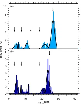
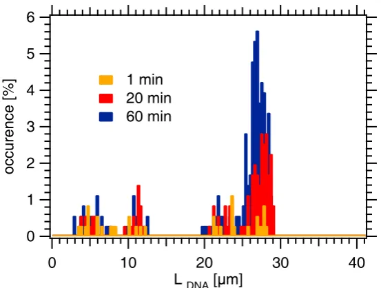
During phage assembly the phage DNA is very tightly packaged into the phage capsid. The question arises if the internal pressure resulting from the high DNA density inside the capsid is responsible for the complete or at least the partial DNA transfer into the host during infection. This was studied for the first time on single T5 phages whose DNA release can be triggered by the receptor protein FhuA in vitro. After T5 phages had adsorbed onto a microfluidic chamber, the ejected DNA was fluorescently stained and stretched in a hydrodynamic flow. The length could thereby be measured continuously. With this setup, we succeeded for the first time in visualizing the dynamics of the DNA ejection in real time. The DNA release is not an all-or-none process but occurs in a stepwise fashion and at a rate reaching 75 000 bp/s. The pauses in between steps can last for over half an hour. The length distribution of the ejected DNA was analyzed and characteristic peaks were found at positions that coincided with the position of single-stranded interruptions (nicks) of the phage genome.
DNA molecules adsorbed onto cationic fluid lipid membranes remain laterally diffusive. During this thesis rectangular grooves of a periodicity of 1000 – 1200 nm and a depth of 40 – 120 nm were imprinted into the thermoplastic “cyclic olefin copolymer” (COC). This substrate was coated with a lipid membrane. The influence of such a support on the conformational behavior of DNA is investigated here. The periodically structured membranes revealed the ability to stretch long DNA molecules. During a collaboration, L. Golubovic provided us with a theory explaining the observed process. The DNA stretching phenomenon can be elucidated in terms of a curvature dependent potential energy attained by the adsorbed DNA molecules.
1 Summary
Zusammenfassung
Im Rahmen dieser Doktorarbeit wurde Desoxyribonukleins¨aure (DNA) in ein-schr¨ankenden Geometrien mit Hilfe von Fluoreszenzmikroskopie untersucht. DNA diente dabei als bekanntes Modellpolymer, das gut mit Hilfe der Polymerphysik beschrieben werden kann. Zum einen wurde die Dynamik des DNA-Austritts aus dem vollgepack-ten Phagencapsids durch den engen Virusschaft untersucht und zum anderen wurden DNA-Str¨ange durch linienf¨ormigen Substratstrukturen manipuliert.
W¨ahrend des Phagenzusammenbaus wird die DNA sehr dicht in das Phagen-capsid gepackt. In dieser Arbeit wurde die Frage untersucht, ob der interne Druck, den die hohe DNA Dichte innerhalb des Capsids verursacht, daf¨ur verantwortlich ist, dass die DNA ganz oder zumindest teilweise w¨ahrend der Infektion in den Wirt transferiert wird. Dies wurde an einzelnen T5 Phagen untersucht, deren DNA Freisetzung man durch die Zugabe des Rezepterproteins FhuA in vitro ausl¨osen kann. Nachdem T5 Phagen auf dem Boden einer Mikrofluidikkammer adsorbiert hatten, wurde die freigesetzte DNA mit Fluoreszenzfarbstoff markiert und im hydrodynamischen Fluß gestreckt. Dadurch konn-te die DNA-L¨ange kontinuierlich gemessen werden. Mit dieser Vorgehensweise gelang es zum ersten Mal die Dynamik der DNA Freisetzung sichtbar zu machen. Diese findet nicht in einem kontinuierlichen Prozess statt, sondern erfolgt schubweise mit Pausen, die ¨
uber eine halbe Stunde dauern k¨onnen. Die Austrittsgeschwindigkeit betr¨agt mindestens 75 000 bp/s. Die L¨angenverteilung der freigesetzten DNA wurde analysiert und dabei wurden charakteristische Maxima bei L¨angen gefunden, die gut mit der Position von einzelstr¨angigen Fehlstellen in der Phagen-DNA, sogenannten Nicks ¨ubereinstimmen.
1 Summary
2 Introduction
A virus that infects only bacteria is called bacteriophage or
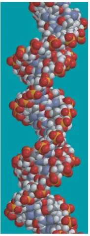
sim-Figure 2.1: DNA
ply phage. The name phage stems from Greek phageton = food/consumption. Phages play an important role in molecular bi-ology as cloning vectors to insert deoxyribose nucleic acid (DNA) into bacteria. DNA contains the genetic instructions specifying the biological development of all cellular forms of life and many viruses. DNA is often referred to as the molecule of heredity, as it is respon-sible for the genetic propagation of most inherited traits. Inserting specific DNA into cells will therefore lead to desired traits of the cells. Additionally, phage therapy has been used as an alternative to antibiotics for treating bacterial infections in the former Soviet Union because phages are highly efficient at killing bacteria. The development of bacterial strains that are resistant to multiple drugs has also led western medical researchers to re-evaluate phages as alternatives to the use of antibiotics. Additionally, some phages seem to be related to human viruses e.g. the phage PRD1 shares a common ancestor with the human adenovirus [1]. Therefore under-standing phages will improve our knowledge about human viruses which is in return helpful for developing effective anti-viral medicine. Like many viruses that infect eukaryotes, phages consist of an outer
protein hull and the enclosed genetic material which consists of double-stranded DNA in 95% of the phages known. In many bacteriophages, DNA is highly compressed (e.g. phage T7: 450 mg/ml [2]) triggering the ongoing discussion on how and why DNA is ar-ranged at such high packing densities [2, 3, 4, 5, 6, 7]. A hypothesis as to why phages pack their DNA so tightly is that the pressure resulting from the tight packing (∼ 50 atm [8]) supplies the energy necessary for the DNA to cross the bacterial cell membrane [9, 10, 11]. In this study, the ejection process of single T5 phage particles is observed in vitro in real time. This allows us to resolve details of the infective process which are not accessible to bulk investigations. Fluorescence microscopy is well suited as a fast and non-invasive technique to observe this process. To resolve the length of the ejected DNA, a fluid flow was applied to stretch it out of its native coiled state.
2 Introduction
in itself. This has been indeed a subject of continuing research (s. chapter 3) for various reasons. The length of DNA can be quite large: a typical human chromosomal DNA strand is a couple of centimeters long. Such long DNA is always coiled and intertwined because of the entropic advantage of such conformations. For most biotechnological applications DNA has to be unfolded since only the uncoiled state allows the correct observation and manipulation of DNA. Additionally, stretching DNA enables us to learn about the mechanical properties of DNA such as its stretching modulus. The mechanical properties of DNA are very important for understanding the physics behind biological processes involving DNA. In typical experiments, DNA is attached with one end to a surface while the other end is pulled [12, 13, 14]. Another common approach to stretch DNA is to use electrostatic or hydrodynamic flow fields [15, 16, 17, 18]. In this work, a novel method to align DNA is presented which is very suitable for potential biotechnological applications. The idea originated from previous work: Cationic lipid DNA complexes form a lamellar structure of alternating lipid membranes and DNA smectic monolayers [19]. The origin of this DNA alignment is thought to originate from a 1-D sinusoidal curvature modulation of the lipid membranes. The DNA is situated within the membrane grooves thereby forming parallel strands [20]. The idea is to reduce this system to 2-D: a supported cationic lipid membrane with adsorbed DNA molecules. The surface curvature of such a supported membrane translates to a resulting attractive or repulsive potential for DNA. The membrane curvature can be achieved by fabricating a grid of parallel grooves on the support of a lipid layer. The surface topography produces attractive and repulsive lines which are shown to orient the DNA molecules similar to the process seen in 3-D. Supported membranes are easily further biofunctionalized [21, 22], thus allowing the use of this system for a broad range of applications, e.g. DNA chips for fast testing of genetic diseases. Standard supports such as mica, glass slides or silicon wafers can be topologically structured, but this requires clean room equipment and it is time consuming. Therefore a simpler method such as imprinting a master into a plastic material would be more desirable. The thermoplastic cyclic olefin copolymer (COC) is ideal for our purposes because its good optical properties [23] allow for the use of high resolution fluorescence microscopy. A theory was developed to describe quantitatively how the DNA stretching process is achieved and how it depends on the charge density of the lipid layer. Finally, the theoretical predictions are compared to the experimental results.
[26, 27, 28, 29, 30, 31]. Typically, supported lipid layers are often only characterized optically, e.g. with fluorescence microscopy or with fluorescence recovery after photo-bleaching which yields the lateral diffusion constant of the lipid molecules [32]. Similar-ily, only a few investigations of supported lipid membranes on hydrophobic substrates were performed and these did not resolve the structure directly [33, 34, 35]. In this thesis it is shown that on hydrophobic COC surfaces lipid layers are organized as thin, loosely packed bilayers. For the first time, optical methods were combined with x-ray reflectivity measurements to characterize charged and neutral lipid membranes supported on COC.
3 The Ongoing Quest to Stretch DNA
DNA is usually organized as two complementary strands, which are held together by hydrogen bonds. Both strands of double stranded DNA (dsDNA) are intertwined to form a double helix, see Fig. 2.1. Such a structural conformation is called B-DNA, which is the natural conformation of DNA. Only very few DNA molecules are not paired in a natural biological environment and form single stranded DNA (ssDNA). A single strand is built from a polyester chain made up of alternating sugar (D-2-deoxyribose) and phosphate groups. A single sugar and phosphate group is called base. The four possible bases are adenine (A), thymine (T), cytosine (C), and guanine (G). Each base “pairs up” with only one other base: A+T and C+G. Therefore the second strand of the double helix DNA is complementary to the first. The specific pairing of the bases is the reason for the unique ability of DNA to replicate itself. The sequence of the different nucleotides translates into a sequence of amino acids which are the building blocks of proteins [36].
In the recent years, a great number of different approaches have been tried to unfold genomic-sized DNA which is naturally coiled and therefore inaccessible for biotechnolog-ical and research methods. For many biotechnologbiotechnolog-ical applications such as optbiotechnolog-ical DNA restriction mapping and sequencing it is necessary to extend the polymer such that a one-to-one mapping can be established between the spatial position along the polymer and the position within the genome [37, 38, 39, 40, 41]. Additionally, it is very difficult to analyze dynamic processes such as the very complex DNA protein interactions if the DNA is folded. Besides, the question how DNA reacts to external forces and restrictions is of essential interest for polymer theorists. Until now, four different approaches to stretch DNA have been applied:
A mechanical force may be applied to one or both ends of the molecule which leads to a constant force acting on each segment of the molecule.
Electrophoretic and hydrodynamic flow can lead to DNA stretching even though the force applied to a segment depends critically on the position within the molecule.
Molecular combing immobilizes stretched DNA molecules on a surface by the vis-cous drag of a receding water surface.
3 The Ongoing Quest to Stretch DNA
3.1 Force Applied to the End of a DNA Molecule
The following techniques may be used to measure force-extension curves of single DNA molecules [42]:
Optical Tweezers: They allow to apply forces between 0.1 pN and 100 pN.
Glass Microneedles: The force can be as small as 1 pN and as large as desired.
AFM: The force ranges between 5 pN and a few nN.
Magnetic Tweezers: They offer a force rage between 0.01 pN and 100 pN.
Which technique is chosen depends on the force range and time resolution needed.
For a physicist, DNA is seen as a heteropolymer whose mechanical behavior can be described by different polymer theories. The genetic information stored in DNA is often not of interest. The details of the molecular structure are neglected and DNA is viewed as a charged cylinder with a diameter of 2.2 nm. Among others, the following models have been developed to describe a polymer reacting to external forces:
Freely-Jointed Chain Model
Worm-Like Chain Model
extensible Worm-Like Chain Model
The freely-jointed chain (FJC) model treats the polymer as a chain of statistically inde-pendent segments of length b (Kuhn length) joined together at the ends. Their orienta-tions are uncorrelated in the absence of external forces. A forceF acting on the free end of a molecule whose other end is attached to a fixed point stretches the polymer as each segment tends to align with the force. The external force is opposed by the thermal agitation of the polymer which tends to disorder the segments. Therefore the elastic response of the molecule with contour lengthL0 is purely entropic and the length of the polymer along the direction of the force (Lz) is given by [12]:
Lz =L0
coth
F b kBT
− F b
kBT
. (3.1)
3.1 Force Applied to the End of a DNA Molecule
Later theoretical analysis showed that the DNA molecule could be described as an elas-tic tube subjected to thermal fluctuations [43]. Its extension is obtained as a balance between the entropy of the molecule and the work of the stretching force. This de-scription, known as the worm-like chain (WLC) model, first introduced by Kratky and Porod [44], turns out to provide an excellent approximation of the elasticity of DNA at forces smaller than ∼15 pN. The WLC model assumes an elastic chain with persistence length ζp and a bending energy per lengthEb =kBT ζpC2/2, wherekB is the Boltzmann constant, T the temperature, and C the local curvature. The following interpolation formula describes the relation between the applied force F and the extension along the axis of the force (z-axis) Lz [43, 45]:
F ζp kBT
= Lz L0 +
1
4(1−Lz/L0)2 − 1
4. (3.2)
However at larger forces (F >15 pN), the DNA molecule no longer responds to the stress by reducing its entropy but by modifying its molecular structure. Near full extension, Lz approaches L0 asF−1/2 [45]. In this regime DNA can also be enthalpically stretched
beyond the contour length defined by B-DNA geometry [13]. An equation that describes this extensible WLC regime well is
Lz
L0 = 1−
1 2
kBT
F ζp 1/2
+F
S , (3.3)
where S is the elastic stretch modulus [46]. The dependence of the persistence lengthζp and the stretch modulus S on salt conditions was investigated by Baumann et al. [47]. For monovalent salt, ζp decreases with increasing salt concentration while S increases. An interpolation formula for an extensible WLC for the complete force range from 0−50 pN was found by Wang et al. [48]:
F ζp
kBT
= Lz L0
+ 1
4(1−Lz/L0+F/S)2 − 1
4−F/S . (3.4)
3 The Ongoing Quest to Stretch DNA
4 1
2 4 10
2 4 100
F [pN]
1.8 1.6
1.4 1.2
1.0 0.8
Lz/L0
S-DNA
B-DNA ssDNA
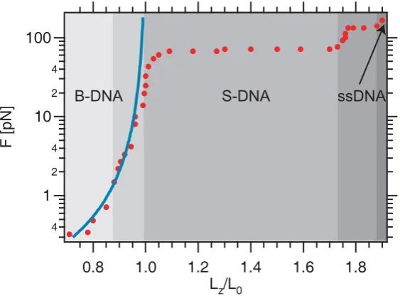
Figure 3.1: Force versus relative extension of dsDNA: Data points are taken from [51] and are shown as red dots. The different regimes are displayed in different shades of grey: The entropic elasticity regime (light grey) is followed by the intrinsic elasticity regime (slightly darker grey). At ∼ 70 pN the DNA makes a transition to S-DNA (grey). At∼150 pN the ds DNA melts (dark grey) and the curve coincides with that of ssDNA (very dark grey). The curve resulting from the WLC model (s. Eq. 3.2) assuming ζp= 50 nm is shown in blue.
in equilibrium. After this transition the force extension curve coincides with that of ssDNA.
Recapitulating, at least five different regimes can be distinguished in the dsDNA force-extension curve (s. Fig. 3.1). At low forces (up to ∼ 15 pN) entropic forces dominate (“entropic elasticity regime”). After that, DNA starts to stretch linearly with F, this “intrinsic elasticity regime” is followed by the transition from the B-type DNA to S-DNA which occurs at 65−70 pN (“overstretching transition”). The DNA may stretch up to 1.7 × its contour length L. At around 150 pN the dsDNA denatures (“melting transition”) and starts to follow the force extension curve of ssDNA.
3.2 Electrophoretic and Hydrodynamic Stretching
3.2 Electrophoretic and Hydrodynamic Stretching
of one part of the chain perturbs the surrounding flow and modifies the hydrodynamic force exerted on another part. Electric fields in aqueous solutions almost always lead to electroosmosis and therefore both hydrodynamic and electric interactions have to be taken into account. Because of the diversity of interactions of DNA with hydrodynamic and electric fields, this overview will be restricted to a few interesting cases.
3.2.1 Tethered DNA in Uniform Flow
Perkins et al. [15] optically trapped a microsphere attached to one end of a DNA molecule while the other end remained free. A uniform (nonshearing) fluid flow was achieved by translating the fluid chamber and therefore also the fluid horizontally with a velocity v while the bead remained stationary. Here, the applied force is zero at the free end and maximal at the attached end. The fractional extension Lz/L0 is a function of ηv L0.54
0 .
η is the fluid viscosity. Surprisingly, over a large extension range (20% to 80%) the relatively simple WLC model (s. Eq. 3.2) coincides with the data very well.
3.2.2 DNA in Shear Flow
The dynamics of flexible polymers in shear flow is of great practical interest because this type of flow occurs whenever a fluid flows past a surface. Smith et al. [16] investigated the behavior of DNA molecules under steady shear flow (dv/dy = γ = const, where y indicates the direction perpendicular to the surface and v is the velocity of the flow). Their data show that even at relatively low shear rates there are large fluctuations in the extension of the molecule. As the shear rateγ is increased the molecules fluctuate more rapidly and reach larger extensions. The mean fraction extension < Lz > /L0 increases gradually with the shear rate and approaches an asymptotic value ofLz/L0 ∼0.4 to 0.5. Doyle et al. [17] observed the dynamics of a single polymer tethered to a planar solid surface in a shear flow using fluorescently labeled DNA chains. Shearing a tethered chain gives rise to large temporal fluctuations in the chain extension. Simulations revealed that these fluctuations are due to a continuous recirculating motion of the chain. This cyclic dynamics was caused by a coupling of the flow field gradient with thermally driven fluctuations of the chain in the shear gradient direction. Ladoux et al. [18] showed that the tethered chains approach full extension as the flow rate was increased very slowly. Assuming a WLC, the shear rate γ is related to the relative extension Lz/L0:
1−Lz/L0 ∼γ−1/3, (3.5)
3 The Ongoing Quest to Stretch DNA
3.2.3 2D Polymer in an Electric Field
B. Maier et al. [52] investigated the elastic response of single DNA molecules to an external electric field in two dimensions. The DNA is tethered at one end to a bead and it is restricted to movements within the 2-D plane of a cationic membrane. The end-to-end distance in the strong stretching limit (νEζp > kBT) elongates with increasing field strength in good agreement with the worm-like chain model adapted to 2D:
Lz ≈1−
1
4νEζpL0
kBT
, (3.6)
where ν is the effective line charge density of the DNA molecule (here: ν = 0.6 ± 0.1 e−/nm) and E the electric field strength.
3.3 Molecular Combing
In a process called “molecular combing” [53, 54], DNA molecules attached at one end to a solid surface were extended and aligned by a receding air-water interface and left to dry on the surface. In contrast to viscous drag and electrophoresis which act on the full length of the molecule, the action of the receding interface appears to be localized at the air-water interface and is thus independent of the length and conformation of the molecule. The combed molecules are lying flat in a linearized state on a dry solid substrate, they are observable with fluorescence even several months after combing, and are available for further manipulation. The force acting on the DNA molecule in the vicinity of the contact line can be estimated by using Hooke’s law. It depends strongly on the surface used to attach the DNA. For silanated surfaces the force amounts to F = 160 pN. This technique has been modified to serve different applications and needs [55].
3.4 Confinement Elongation
3.4 Confinement Elongation
Self avoidance effectively divides the confined polymer into a series of noninterpene-trating blobs, distributing the polymer mass along the channel in such a way that the monomer density is uniform. Consequently the extension of the polymer in the channel Lz must scale linearly with the contour length L0 [57]:
Lz L0
(ζpw)1/3
d2/3 , (3.7)
where w is the width of the polymer (here 2 nm) andζp the persistence length (50 nm). Once the channel dimensions drop below the persistence length, the de Gennes approx-imation fails and the following approxapprox-imation of Odijk has to be considered [58, 59, 60]:
Lz =L ⎡
⎣1−0.361
d ζp
2/3⎤
⎦ . (3.8)
4 About Lipids and Membranes
4.1 Biomembranes
Life as we know it is only possible because nature has invented membranes. Membranes enable the separation of living entities from the lifeless and possible hostile environment while preserving a selective material exchange between the two worlds. Additionally, the function of cells, the basic unit of life, depends on the controlled interplay between compartments performing different functions. Therefore, membranes are used to divide the cell into compartments which are specialized for certain well defined functions. Si-multaneously, the biomembranes themselves developed into sites of essential biochemical functions, such as protein biosynthesis or oxidative phosphorylation. Therefore the in-tracellular space is divided into two sub-spaces: the lumina of the various organelles and the cytosol. For example, different ionic compositions and pHs can be established in the lumina of the various organelles essential for varying purposes. Membranes differ in molecular composition and architecture according to the function of the compartment they are enveloping. For example, the cell membrane (plasma membrane) of animal cells is in general a three layered compound system (see Fig. 4.1). Its center is formed by a
Figure 4.1: Schematic illustration of a typical plasma membrane, in this case an erythrocyte membrane. Image taken from [62].
4 About Lipids and Membranes
by the oligosaccharides protruding from glycolipids or proteins. At the intracellular side the membrane is coupled to the cytoskeleton, a stabilizing protein complex [63]. The fundamental component of all biomembranes is the lipid bilayer, which consists of two monolayers of lipids facing each other. Proteins are embedded into the fluid, i.e. freely diffusive lipid matrix [64].
4.2 Lipids
The term lipid comprises a diverse range of molecules such as fatty-acid derived phospho-lipids, sphingophospho-lipids, glycolipids and terpenoids, such as retinoids and steroids. Mem-brane lipids consist of a polar, hydrophilic headgroup and nonpolar, hydrophobic tails. This amphiphilic nature of lipids is responsible for their self assembly properties. The hydrophobic tails tend to be packed together away from the water surrounding while lipid heads face towards it. Therefore, lipids will aggregate in aqueous environments if a certain lipid concentration called critical micelle concentration is exceeded. Among a variety of structures lipids may form micelles, vesicles or bilayer structures depend-ing on the exact size relation of the hydrophobic to the hydrophilic part of the lipid. Cone-shaped molecules tend to form micelles while cylindrical molecules prefer to form bilayers. A bilayer consists of two monolayers of lipids where the hydrophobic tails face each other and the hydrophilic heads shield them from the surrounding water. This structure is also called a membrane and is the fundamental structure of biomembranes. Multiple membranes stacked on top of each other and separated by thin water layers are referred to as the lamellar or multilamellar phase.
4.2 Lipids
O O
O O
O P
O
O
O
NH3+
-fatty acid residue: palmityl
fatty acid residue: oleoyl
glycerol residue
phosphoric acid residue
alcohol: ethanol-amine
unpolar part: lipid tails polar part: lipid head
Figure 4.2: Structure formula of the phosphoglycerollipid POPE. The two fatty acids (here palmitoyl and oleoyl) are esterified to the hydroxyl groups of the glycerol backbone. The phosphate group is attached to the glycerol backbone by an ester link. This group is finally linked to an alcohol, such as ethanolamine (shown here) or inositol, serine or choline.
A lipid bilayer can undergo multiple phase transitions upon heating. The chain-melting transition or the gel to liquid crystalline phase transition is accompanied by the largest entropy change. The bilayer changes from the gel phase to the liquid-crystalline phase (Lα) (s. Fig. 4.3 (a)) at the main transition temperature (Tm). The gel phase comprises
(a) Lα (b) Lβ' (c) Pβ' (d) Lc
Figure 4.3: Different lipid bilayer phases: (a) Lα phase, the bilayer is fluid and the lipid chains are unordered. (b) Lβ phase, the bilayer is in the ordered gel phase, the chain orientation is tilted with respect to the membrane normal. (c) The ripple phase (Pβ). The membrane shows a saw tooth like height variation. (d) The
liquid-crystalline phase: the lipids are immobile and ordered.
4 About Lipids and Membranes
freely within the bilayer. The corresponding diffusion coefficients usually are between 1−10µm2/s.
4.3 Structural Models of Substrate Supported
Membranes
Lipids can interact in several ways with surfaces [s. Fig. 4.4]. If the substrate is too rough or chemically heterogeneous, no lipid adsorption is expected [33]. For hydrophilic
(a)
Vesicles
(e)
Bilayer
(b)
(c)
(d)
Monolayer
(f)
Trilayer
Figure 4.4: Coating Possibilities: Schematic drawing of how the lipids might coat the COC surface: (a) lipid vesicles attached to the surface (b) monolayer with the lipids laying flat on the substrate (c) monolayer with the lipid tails inserted into the substrate (d) monolayer with the tails facing towards the surface (e) lipid bilayer (f) trilayer: a bilayer is firmly attached to a lipid monolayer on COC.
4.3 Structural Models of Substrate Supported Membranes
5 Preparation Techniques and
Experimental Methods
5.1 Materials and Preparation Techniques
Chemicals 1,2-Dioleoyl-sn-Glycero-3-Phosphocholine (DOPC) [Fig. 5.1 (a)] and 1,2-Dioleoyl-3-Trimethylammonium-Propane (DOTAP) [Fig. 5.1 (b)] were bought from Avanti Polar Lipids Inc. (Alabaster, USA) and used without further purification.
2-(12-(7-nitrobenz-2-oxa-1,3-diazol-4-yl)amino)dodecanoyl-1-hexadecanoyl-sn-glycero-(a) DOPC
(b) DOTAP
5 Preparation Techniques and Experimental Methods
3-phosphocholine (NBD C12-HPC) was purchased from Molecular Probes (Eugene, USA). For diffusivity measurements, 1% (w/w) of the fluorescence probe was used to label the membrane. For the experiments with DNA, the lipids were mixed with 0.05% (w/w) of 2-(4,4-difluoro-5-(4-phenyl-1,3-butadienyl)-4-bora-3a,4a-diaza-s-indacene-3-pentanoyl)-1-hexadecanoyl-sn-glycero-3-phosphocholine (Bodipy-C5HPC, Molecular Probes, Eugene, USA).
Only freshly bidistilled water (18.2 MΩ, Millipore, Billerica, USA) was used throughout this study.
Chloroform, toluene and 2-propanol were bought at HPLC grade from Carl Roth GmbH & Co (Karlsruhe, Germany).
N-(2-Hydroxyethyl)piperazine-N’-(2-ethanesulfonic acid) (HEPES), tris(hydroxyl-methyl)aminomethane (TRIS), CaCl2, MgSO4, NaCl, ascorbic acid (vitamin C), ethylene-ediamine-tetraacetic acid (EDTA), H2O2, and NH4OH were bought from Sigma Aldrich (Taufkirchen, M¨unchen) at a purity of 99.5%. N-octyl beta-D-glucoside (octyl glycoside, OG) was purchased from Bachem (Basel, Switzerland).
The DNA intercalating dyes, 1-1’-[1,3-propanediylbis[(dimethyliminio)-3,1-propane-diyl]]bis[4-[(3-methyl-2(3H)-benzothiazolylidene)methyl]]-tetraiodide (TOTO-1) and 4-[(3-methyl-2(3H)-benzoxazolylidene)methyl]-1-[3-(trimethylammonio)propyl]-,di-iodide (YO-PRO-1), were bought from Molecular Probes (Eugene, USA).
Buffer Solutions For the phage experiments, the following buffer solutions were needed:
phage buffer: 10 mM Tris-HCl, 100 mM NaCl, 1 mM MgSO4, and 1 mM CaCl2 (pH 7.6)
flow buffer: 10 mM Tris-HCl, 100 mM NaCl, 1 mM MgSO4, and 1 mM CaCl2 0.1µM YO-PRO-1 and 0.01% OG (pH 7.6)
OG buffer: 25 mM HEPES, 150 mM NaCl, OG 0.5% (w/v) (pH 7.4)
For the DNA experiments the following buffers were prepared:
attachment buffer: 10 mM Hepes (pH 7.0)
salt buffer: 10 mM Hepes, 30 mM NaCl, 5 mM Vit C (pH 7.0)
DNA storage buffer: 10 mM Tris, 1 mM EDTA (pH 7.5) (TE buffer)
5.1 Materials and Preparation Techniques
DNA λ-phage DNA (48 502 bp) was bought from Roche (Mannheim, Germany), di-luted to a concentration of 0.1µg/ml in DNA storage buffer and stored at -20◦C. 127µl of a 0.5µM Toto-1 solution and 1 ml of the attachment buffer were added to 200µl of DNA. The solution was heated to 50◦C for 20 min. This results in a labelling ratio of 1:5. Pipet tips were cut to avoid high shear forces during DNA handling.
Microfluidic Chambers The plastic chambers (µ-Slides, ibidi GmbH, M¨unchen, Germany) consisted of two reservoirs connected by a channel with dimensions 5 x 0.4 x 50 mm3 (width×height×length). The bottom of the channel was sealed with a plastic foil made out of the copolymer 2-norbornene ethylene (cyclic olefin copoly-mer, COC). Its high transparency and the thickness of 0.18 mm allow the application of high resolution optical microscopy ([Fig. 5.2 (a)]. The microfluidic chambers were cleaned before use by flushing 2 ml of 2-propanol through the flow chamber followed by at least 20 ml of bidistilled water. For the x-ray reflectivity measurements, a thin film
(b)
Si wafer coated with COC
microscope objective
x-ray
(a)
microscope objective
COC foil channel
Figure 5.2: Microfluidic Chambers: (a) Schematic drawing of the plastic chamber used for microscopy (side view). (b) Modified chamber for the x-ray measurements (side view).
of COC was prepared by spin-coating COC onto a silicon wafer thus avoiding the long range undulations present in free-standing foils. A silicon wafer (20×20 mm2) with a thermally grown oxide layer of 400 nm thickness was cleaned thoroughly for the COC coating by a modified RCA method [69]. In short, the wafer was ultrasonicated for 5 min in acetone, in 2-propanol, and in water. Afterwards it was boiled at 80◦C in a 1:1:5 H2O2:NH4OH:H2O mixture. The wafer was shortly rinsed in bidistilled water, then boiled in 1:1:5 H2O2:HCl:H2O at 80◦C. The wafer was dried at 70◦C for 3 hours. 300µl of 1 mg/100 ml COC dissolved in toluene was deposited onto the wafer and the wafer accelerated to 3000 rpm for 2 min. This procedure yielded a homogeneous, smooth COC layer with a thickness of around 450 ˚A and a surface roughness of 7 ˚A.
5 Preparation Techniques and Experimental Methods
the channel interior. Finally the chamber was sealed again with a two component epoxy glue (“Uhu Plus Endfest 300”, Uhu GmbH, B¨uhl, Germany) [Fig. 5.2 (b)]. After drying for several hours, the chamber was ready for the deposition of the lipids.
Assuming a Poiseuille flow, the volume flow rate can be related to the shear rate at the bottom of the chamber by γ = 6Φ/wh2 (w = 5 mm width of chamber, h = 0.4 mm height of chamber). We flushed up to 8 ml/min through the channel resulting in a shear rate of roughly 1000 s−1.
The patterned COC surface used in the DNA experiments were produced the following way:
The grating substrates were produced using holographic methods and subsequent reac-tive ion etching techniques on (100) silicon wafers (25 ˚A of native oxide)[71]. To imprint the negative structure on COC [72], the waver was put onto a COC foil with a weight of 80 g. The temperature was raised to 150◦C and the sample equilibrated over night (s. Fig. 5.3). The master was removed after the temperature had dropped below 70◦C[73]. The foil was glued to the µ-slide top part with the patterned surface facing into the channel.
silicon master
COC
Figure 5.3: : Imprinting: the silicon master is pushed onto the planar COC foil while the temperature is raised to 150◦C.
5.2 Methods
Vesicle Fusion (VF) The desired lipid ratio was mixed in chloroform, dried under nitrogen flow, and stored in a vacuum chamber over night. Bidistilled water was added to the dried lipid to a concentration of 1 mg/ml and the solution was incubated for 4 h at 50◦C resulting in multilamellar vesicles. Small unilamellar vesicles were prepared by sonicating the lipid-water mixture in a tip sonicator (Sonoplus UW 2070, Bandelin electronic, Berlin, Germany) for 10 min at an amplitude of 170µm while the solution was cooled on ice [74]. 400µl of the lipid solution were deposited into the chamber channel and incubated over night. The chamber was washed with at least 100 ml of bidistilled water while great care was taken to avoid air contact with the lipid layer.
Solvent Exchange (SE) The lipids were mixed and dried as described above. A solution with a concentration of 1 mg/ml was prepared by adding 2-propanol to the dried lipid. 200µl of the lipid solution were injected to the chamber. 2 ml of bidistilled water were added into one of the two reservoirs of the chamber which lead to a reduction of the 2-propanol content in the solvent to 10%. After equilibration of the water levels in both reservoirs, 30 ml of bidistilled water were quickly flushed through the plastic slide to remove excess vesicles in the buffer solution and reduce the amount of vesicles adhered to the membrane.
For comparison, a membrane on a hydrogen-terminated silicon wafer (H-Si) was prepared as follows: a DOPC membrane was deposited by spin coating a DOPC 2-propanol solution (1 mg/ml) immediately after a HF etch [30]. Then the dried sample was placed in the microfluidic chamber and flushed with water prior to the measurement.
T5 Phage Wild-type T5 (wt) and T5 st(0), a heat stable deletion mutant, were used throughout this study. They were produced on E. coli Fsuβ+ and purified by polyethy-lene glycol precipitation followed by a CsCl-step gradient as described in Bonhivers et al. [75]. They were stored in phage buffer at a concentration of 1013 phage particles/ml at 4◦C.
FhuA was overexpressed in E. coli HO830fhuA transformed with plasmid pHX405 and purified following the protocol descibed in Boulanger et al. [76]. The protein was solu-bilized in OG buffer and stored at 4◦C at a concentration of 2 mg/ml.
5.2 Methods
5.2.1 Fluorescence Microscopy
5 Preparation Techniques and Experimental Methods
explanations. The exited electron of the fluorochrome relaxes very fast from higher rotational and vibrational states to the lowest exited state (S1). From this state the electron can return to the ground state (S0) or to some vibrational state above it while emitting a red-shifted photon. In rare cases, the electron undergoes intersystem crossing to the triplet state from where it also returns to the ground state by emitting a red shifted photon (phosphorescence). A sample labeled with a fluorescence probe is illuminated
S1
S0
T1
Figure 5.4: Simplified Jablonski diagram showing the possible transitions of a fluo-rochrome. By photon absorption the electron is lifted from the ground state S0 to an exited state S1. The electron relaxes back to the ground state by emitting a photon of reduced energy. In rare cases the electron can perform the so called intersystem crossing and ends up in the triplet state T1 from where it can relax back to the ground state by releasing a photon (phosphorescence).
with light within the absorption wavelength range. The emitted red-shifted fluorescence light is collected with an objective which creates a sharp image of the fluorochrome distribution in the sample. This image can be detected with a CCD camera or it might be seen with the eyes with the help of ocular lenses. In this study, an epi-fluorescence setup was used, i.e. the excitation light is steered through the same objective lenses that are used for the collection of the emitted light.
Experimental Details Fluorescence microscopy was performed on an inverted fluores-cence microscope (Axiovert 100M, Carl Zeiss, Oberkochen, Germany) equipped with an 100×oil immersion objective (100 Plan Neofluar, N.A. 1.3, Carl Zeiss, Oberkochen, Ger-many). Images were captured with a CCD camera (CoolSnap HQ, Photometrics, Roper Scientific Inc., Tuscon, USA) and analyzed with Igor Pro 4.0 (Wavemetrics, Portland, USA).
5.2.2 Continuous Bleaching
5.2 Methods
closed in such a way that only a roughly circular spot ( 70µm) is illuminated while the rest of the membrane is left in the dark.
In the center of the observation area, the fluorescence signal of the membrane decays exponentially as a function of exposure time as expected for a large ensemble of contin-uously exited dyes:
I(x=d/2, t) = Id/2 e−bt+B . (5.1)
Here I(x, t) is the intensity, x is the distance from the rim towards the center of the illuminated area, d is the diameter of the field stop, t is the time since the beginning of the exposure,B is the background noise, andb is the bleaching constant, which depends on the brightness of the illumination, the buffer, and on the fluorescent molecule used.
At the edge of the illuminated area, two cases have to be taken into account. If the membrane is immobile, a discontinuous jump in the concentration of unbleached dyes forms at the edge of the illuminated area. If the lipid layer is fluid, unbleached fluo-rescently labeled lipids from the surrounding non-illuminated area diffuse continuously into the illuminated spot thereby increasing the fluorescence signal at the rim. Hence, a bright halo forms at the periphery of the illuminated area. In this case, the signal decreases approximately exponentially from the dark field stop towards the middle of the observation area:
I(x, t0) =It0 e−x/λ+B =It0 e− √
b/D x+B , (5.2)
where λ is the decay length, D = b/λ2 is the diffusion constant of the lipid layer, and b is the bleaching constant. Equation 5.2 holds only for small x. If x is too large, the decaying fluorescence signal is obscured by the background. It is important that an equilibrium between the bleaching process and the diffusion process is established. Care has to be taken that the sample is not bleached too much for having a good signal to noise ratio. Both conditions are met within 5 ≤tb≤10.
5.2.3 Fluorescence Recovery After Photobleaching
5 Preparation Techniques and Experimental Methods
Here, only the theory concerning the transport by diffusion monitored with an uniform circular laser profile will be described. It is thus possible to determine the diffusion constant D and the mobile fraction M of the fluorophore.
The bleaching intensity I(r) is given by
I(r) =
P0
πω2 : r ≤ω
0 : r > ω , (5.3)
whereP0 is the laser power, ω the beam radius, andr is the distance from the center of the bleaching spot. If the photobleaching of the fluorophore is an irreversible first-order reaction with rate constant α, the concentration of the unbleached fluorophore C(r, t) can be calculated from
dC(r, t)
dt =−αI(r)C(r, t). (5.4)
The concentration immediately after bleaching at t = 0 is given by
C(r,0) =C0exp (−αT I(r)) , (5.5)
whereC0 is the initial uniform fluorophore concentration. T is the bleaching time which should be short compared to the characteristic time of diffusion τD. The concentration is determined by the following diffusion equation:
∂C(r, t)
∂t =D∆C(r, t). (5.6)
If the solution is denoted as CK(r, t), the fluorescence signal F(t) at t ≥ 0 can be represented by
FK(t) = q
A I(r)CK(r, t)d
2r , (5.7)
whereqis the combined quantum efficiency of absorption and emission andAthe atten-uation factor. To simplify the mathematic description, it is more convenient to display a fluorescence recovery curve in the fractional form
fK(t) =
[FK(t)−FK(0)]
5.2 Methods
Here, the fractional recovery curve can be described as
fK(t) = 1−(τD
t )exp
−2τD
t
[I0(2τD
t ) +I2( 2τD
t )]
∓ 2
∞
k=0
(−1)k(2k+ 2)! (k+ 1)!(τD
t )k+2
(k!)2[(k+ 2)!]2 , (5.9)
where τD = 4ω2
D [78]. The mobile fraction M can be determined quantitatively from the
recovery ratio
M = FK(∞)−FK(0) FK(−)−FK(0)
, (5.10)
whereFK(−) is the fluorescence signal before bleaching. If one considers the diffusion of bleached fluorophores to the outside of the spot, the following equation can be derived [79]:
FK(t) = FK(∞)−
[FK(−)−FK(0)]·
{1−exp −2τD
t
[I0(2τD
t ) +I1( 2τD
t )]}. (5.11)
This equation was used to fit the experimental data. The parameter are used to extract D and M.
5 Preparation Techniques and Experimental Methods
5.2.4 X-ray Reflectivity
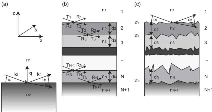
Theory of Specular X-Ray Reflectivity Specular x-ray reflectivity can be described with the laws of classical optics if the appropriate index of refraction n is used. For x-rays, n= 1−δ−iβ, with the dispersion δ and the adsorptionβ:
δ = r0 2πλ
2ρ and (5.12)
β = λ
4πµ . (5.13)
λ is the wavelength of the incident wave, re the electron radius, which is also known as the Thompson scattering length of the electron. ρ is the electron density and µ the linear absorption coefficient.
(a) (b) (c)
αi αf
αt
αi αf
αt 1 2 3 ... N n1 n2 n3 nN n1 n2 n3 nN 1 2 3 ... N d2
ki kf
d3 dN d2 d3 σN σ2 σ1 n1 n2 N+1 nN+1
nN+1 N+1
dN T1 R1
R2 T2 T2 R2 R3 T3
TN-1RN-1
RN TN TN RN
TN+1 z
x y
q
Figure 5.5: X-Ray Reflectivity: (a) The incident wave is scattered at a perfectly smooth surface resulting in a reflected beam and a transmitted beam whereαi=αf
and cosαt = nn12 cosαi. (b) Sketch of a system consisting of N+1 layers with N
interfaces. (c) Same multilayered system, now including interface roughnesses.
For a single interface between two media with the refractive indices n1 and n2 an in-coming electromagnetic wave with wavevector ki (|ki| = 2λπ) is splitted into a reflected (αi = αf) and a transmitted wave with an angle αt (cosαt = n1
n2 cosαi) (Fig. 5.5 (a)).
5.2 Methods
reflected x-ray wave (“Fresnel Reflectivity”) can be analytically determined from Fres-nel’s equations. Total external reflection occurs if n1 < n2 and αi < αc =
2(δ2−δ2). For αi >3αc, RF can be approximated by RF = (αc/2αi)4.
For practical applications, the case of multiple interfaces is more interesting than that of a single surface. Fig. 5.5 (b) shows a multilayer stack consisting of N interfaces. Scattering from all interfaces has to be taken into account. The recursion algorithm described in the classic paper of Parrat et al. [80] allows to calculate the reflection and transmission coefficients (Rj and Tj) of the jth interface from Rj−1 and Tj−1 of the preceeding interface. Assuming that the reflectivity of the substrate RN+1 is zero and that T1 = 1 all reflectivity coefficients can be calculated, arriving finally at R1, the measured reflectivity.
In practice, interfaces are always rough. Therefore the measured reflectivity will be significantly lower than the intensity calculated in the previous paragraph. Instead of looking at a constant refractive index n with sharp steps it is now preferable to think of a continuous refractive index n(x, y, z). Since the moment transfer q = ki −kf (|q|= 4π
λ sin(αi)) is parallel to the z axis, which is perpendicular to the sample surface,
one-dimensional refractive index profiles are considered:
nj =
nj(x, y, z)dy dx. (5.14)
with σj being the surface roughness of the jth interface. The refractive index profile in between the layers j and j + 1 is assumed to be:
nj(z) = nj
+nj+1
2 −
nj−nj+1
2 erf
z−zj
√ 2σj
. (5.15)
The recursive algorithm can now be modified accordingly, yielding the final reflectivity R1.
5 Preparation Techniques and Experimental Methods
setup are described in Reich et al. [70]. Special care was taken to avoid beam damage due to overexposure by shifting the sample during the measurement. Since all reflectivity curves could be reproduced with a high accuracy during several consecutive scans, we can exclude beam damage. The data were analyzed using the Parratt algorithm [80].
channel
copper support substrate
plastic chamber
(a) (b)
chamber
l d α
COC foil
SiO2 water
Figure 5.6: X-Ray Reflectivity: (a) Photo of a microfluidic chamber used during the experiments. The chamber is inserted in a copper block to stabilize it during reflectivity experiments. (b) Schematic drawing of a cross section along the plane of incidence: The incoming beam travels through the length l of the plastic material COC and then the lengthdthrough the bulk water. The reflectivity data is corrected for the resulting attenuation.
5.2.5 Atomic Force Microscopy
(b) (a)
Figure 5.7: Schematic setup of Atomic Force Microscopy (AFM). A sharp tip at-tached to a cantilever is pulled over a surface. Height undulations lead to deflection of the cantilever which is registered by the movement of a reflected laser beam.
5.2 Methods
beam is reflected from the cantilever and variations of the position of the reflected beam are measured by a quadrant diode (Fig. 5.7). Atomic Force Microscopy (AFM) pictures were taken on a NanoScope MultiMode AFM (Digital Instruments, Santa Barbara, USA) in contact mode with a constant force and 512 dots per line and 512 lines.
5.2.6 Scanning Electron Microscopy
An electron microscope uses electrons with a deBroglie wavelength λ =h/√2meeU to resolve structural details of a sample. Here, me is the electron mass, e is the electron charge, and U is the voltage used to accelerate the electron beam. The electron beam is created in the electron gun and accelerated to the desired voltage. The electron beam is collimated by electromagnetic lenses and focused to a very fine spot. The scanning coils deflect the electron beam such that the electron beam is moved back and forth across the specimen. The electron beam hits the surface and frees electrons from the sample. This electrons are detected and an image is generated.
A field emission scanning electron microscope (Modell DSM 982 Gemini, LEO Elek-tronenmikroskopie GmbH, Oberkochen, Germany) was used to image both the gold sputtered imprinted foil and the original master at 5 keV.
condensing lenses
scanning coil
objective lens
target
detector
electron gun
6 Real-Time Imaging of DNA Ejection
from Single Phage Particles
6.1 Introduction to T5 Phage
Bacterial viruses or bacteriophages, frequently called “phages”, were discovered at the beginning of the twentieth century. Bacteriophages constitute one order, 13 families, and 30 genera which is a proof of their diversity. Tailed dsDNA phages (Caudovirales) consist
50 nm
Figure 6.1: Electron microscopy images of different phages. Image taken from reference [81].
of an isometric proteinaceous capsid in which the viral genome is condensed [2]. Located at one of the capsid vertices is an oligomeric protein structure, the connector, that links the capsid to the tail and forms the channel through which the DNA is packaged during morphogenesis and exits during infection [82]. The tail ends with fibers and a tail tip that ensures the binding of the phage to a specific host membrane receptor.
6 Real-Time Imaging of DNA Ejection from Single Phage Particles
structure of the peptidoglycan. Infection results after a phage particle has reversibly bound to liposaccharides of the E. coli outer membrane with its tails fibers. The phage irreversibly binds to the membrane protein FhA with pb5, a protein located at the distal end of the phage tail. FhuA is an outer membrane protein ofE. coli that transports iron chelated to the siderophore ferrichrome [76]. Upon infection, receptor binding leads to conformational changes that are transmitted to the connector triggering its opening and the release of the DNA, which is transferred to the cytoplasm linearly base pair after base pair through the bacterial envelope (reviewed in [83] and [84]). The T5 infectious
100 nm
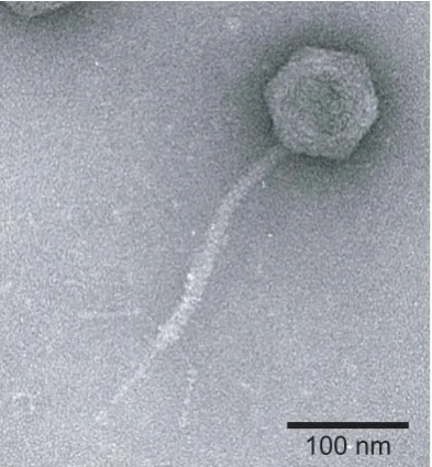
Figure 6.2: Electron microscopy image of a T5 phage virion. Image taken at the Institut de Biochimie et Biophysique Moleculaire et Cellulaire, UMR, CNRS at Uni-versit´e Paris Sud. Permission for publication granted by L. Letellier.
cycle lasts roughly 20 min during which about 200 new phages are produced. Its DNA (121.4 kbp, 41.3µm) may be released from the capsid in vitro by mere interaction of the phage with its purified Escherichia coli outer membrane protein receptor, FhuA [75, 85, 86].
6.2 Setup
6.2 Setup
a fluorescence microscope. The experimental setup is shown schematically in Fig. 6.3. The best results were obtained for the following experimental conditions:
microscope objective
Figure 6.3: Schematic drawing of the experiment: Phage particles (red hexagons) adsorb to the COC surface in the microfluidic slide. The phage DNA is stained with an intercalating dye (yellow stars). The injection of the receptor protein FhA (green dots) triggers the ejection of the phage DNA. The partly ejected DNA is stretched by an applied hydrodynamic flow (depicted as black arrows). The ejection process can now be monitored with a fluorescence microscope.
Adsorption Procedure 150µl of a phage solution containing 6×10⁶particles/ml were incubated for 5 min in the microfluidic chamber to allow the T5 phage particles to adsorb to the bottom of the microfluidic chamber. We found that the amount of attached phages did not increase further when the incubation time was prolonged to as much as one hour.
The concentration of attached phages was roughly proportional to the phage con-centration during incubation. Therefore we chose a incubation concon-centration that resulted in a phage surface density that allowed to observe several phages at once which improved the statistics while still keeping the probability low that two phages attached too close together to be resolved separately.
The phage particles resisted continuous perfusion with the flow buffer up to a flow velocity of 10 ml/min for more than one hour without being detached (data not shown). Therefore we conclude that the phage particles were strongly bound to the surface.
6 Real-Time Imaging of DNA Ejection from Single Phage Particles
bright spots corresponding to individual phage particles that were either stained by the diffusion of the dye through the capsid or by staining of the capsid itself. This allowed us to focus onto the surface before the ejection was started. The YO-PRO-1 concentration was chosen such as to obtain a reasonable fluorescence signal while avoiding quenching effects.
Flow Buffer Low concentrations of the surfactant octyl glucoside (OG) had a protective effect against photobleaching and DNA breaking usually induced by intercalating dyes [87]. High amounts of OG lead to air bubbles in the flow buffer which tore apart the phages. This lead to a release of DNA which sticked irreversibly to the surface. A concentration of 0.01% OG in the flow buffer turned out to provide optimal results.
It was necessary to keep the concentration of the intercalating dye YO-PRO-1 at 0.1µM during the stretching because the DNA fluorescence would eventually subside without it. An explanation of why the fluorescence signal deteriorated without YO-PRO-1 in the flow buffer is given in the following: Since the dye is not covalently bound to the DNA, it does have a considerable on/off kinetic. Unbound dye molecules will be swept away immediately when a flow is applied and can not be replenished if the flow buffer does not contain the dye.
Strength of Flow To resolve the ejection process with the fluorescence microscope it was necessary to stretch the partly ejected phage DNA. Without a flow the DNA builds a random coil where the contour length cannot be resolved with optical microscopy. The flow should stretch the DNA reasonably while not exerting too high force on it to avoid overstretching. Details will be discussed in the next chapter.
Illumination The illumination of the sample had to be carefully controlled to avoid bleaching and breaking of the exposed DNA molecules as observed previously with this family of intercalating dyes [87] while still allowing the detection of single DNA molecules. Therefore the illumination was reduced to 6% by a neutral density filter.
6.3 Response of the Ejected DNA to a Hydrodynamic Flow of Variable Strength
6.3 Response of the Ejected DNA to a Hydrodynamic
Flow of Variable Strength
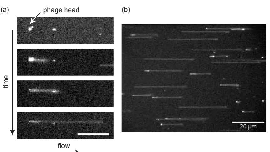
DNA stretching by flow is completely reversible. Without flow the DNA forms a random coil (Fig. 6.4 (a)). The same DNA can be stretched to the left (Fig. 6.4 (b)) and right (Fig. 6.4 (c)). The extension of partly ejected DNA was measured at varying strengths
no flow (a)
phage head
(b)
(c)
Figure 6.4: Fluorescence microscopy pictures of a single phage particle with partly ejected DNA. The white bar has a size of 10µm. (a) No flow is applied, the DNA is in a random coil conformation. (b) A flow is applied which stretches the DNA to the left or (c) to the right.
of the flow. Accurate measurements required to know how much the intercalating dye increased the mean basepair distance. We assumed that YO-PRO-1 intercalation leads to an overestimation of the DNA length by a factor of approximately 1.2 [52]. The measured DNA length was divided by this factor to gain a extension per basepair of 0.34 nm which corresponds to a contour length of 41.2µm of the complete T5 phage DNA. Fig. 6.5 displays the length Lz of four representative DNA strands versus the applied flowΦafter applying the correction for the intercalating dye. The DNA length increased monotonically with the flow and reached a plateau for flows higher than 2 ml/min (shear rate: 250 s−1, see 5.1). For the extrapolation of the plateau value L0 the data was fitted with the relation:
Lz =L0
1−(CΦ)−1/3, (6.1)
6 Real-Time Imaging of DNA Ejection from Single Phage Particles 0.1 2 3 4 5 6
1 - L
z
/L0
0.1 2 4 6 81 2 4 6 810 Φ [ml/min]
40 30 20 10 0 L z
[µm] 10 8 6 4 2 0
Φ [ml/min]
(a) (b)
Figure 6.5: Length of ejected DNA versus applied flow: (a) The length of the ejected DNA is plotted for different phages versus the applied flow. From the fitted curves (solid lines) the plateau value, the contour length, can be derived. By measuring at a flow velocity of 0.6 ml/min, the contour length is underestimated by a factor of 1.3. (b) 1−Lz/L0 is plotted for the same four viruses versus the flow rate in a log-log
graph. The expected slope of−1/3 is shown as a black solid line which describes the data accurately.
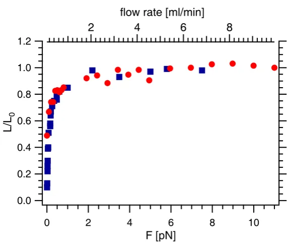
extensionL/L0 versus the flow and compared the curve obtained with the force-extension curve of a DNA molecule to whose end a force is applied [88] (Fig. 6.5). Because both curves overlap, it may be deduced that a maximum force of 10 pN was applied under our experimental conditions. Further experiments were performed at flow rates of 0.5 to 0.6 ml/min which corresponds to a force of about 2 pN. Therefore the measured lengths needed to be corrected by a factor or 1.3 to compensate for the incomplete extension.