An Efficient and Leightweight Illumination model for
Planetary Bodies including Direct and Diffuse Radiation
Marco Scharringhausen
German Aerospace Center
Institute of Space Systems
Bremen, Germany
Lars Witte
German Aerospace Center
Institute of Space Systems
Bremen, Germany
12. April 2018
Zusammenfassung
We present a numerical illumination model to calculate direct as well as diffuse or Hapke scattered radiation scenarios on arbitrary planetary surfaces. This includes small body surfaces such as main belt asteroids as well as e.g. the lunar surface. The model is based on the raytracing method. This method is not restricted to spherical or ellipsiodal shapes but digital terrain data of arbitrary spatial resolution can be fed into the model. Solar radiation is the source of direct radiation, wavelength-dependent effects (e.g. albedo) can be accounted for. Mutual illumination of individual bodies in implemented (e.g. in binary or multiple systems) as well as self-illumination (e.g. crater floors by crater walls) by diffuse or Hapke radiation. The model is validated by statistical methods. Aχ2test is undertaken to compare simnulated images with DAWN images acquired during the survey phase at small body 4 Vesta.
1
Introduction
Reliable prediction or at least estimation of illumination conditions on the surface of plane-tary bides (e.g. the Earth moon) or small bodies like asteroids or comet cores is essential for mission planning purposes.
In general, mission planning for any vehicle on a strategic (before start of the mission) and/or tactical level (during the mission) requires knowledge about environmental conditions at the destination. From a general point of view and depending on the vehicle(s) involved, this might include atmospheric properties such as density, wind speed as well as surface properties such as roughness, slope, gravity and illumination. This applies not only to surface elements but also to planetary landers.
Firstly, thermal design of any lander space craft relies on a reliable information about the environment (e.g. [2]). As solar radiation is in general the major source of energy on the surface of a small, atmosphereless body in space, a simulation suite for calculation of the surface radiative intensity delivers boundary conditions for any thermal model of the surface. The same applies to the design of a mobile surface element powered by solar cells, e.g. a rover. For rovers, additional aspects come into play, i.e. not only the thermal and power budget are affected by illumination conditions but also the path and trajectory planning of the rover itself ([14], [7]). Being able to reliably predict illumination at any time and at any point on the surface of the small or planetary body is an essential part of the cost function in any optimization process. During the mission, the rover’s mission plan may involve travel to several distinct sites, interleaving periods of dedicated science data collection with periods of traversal and opportunistic science. To repower internal batteries, it might be beneficial to pause for a period of time to exploit time slots of maximal illumination. To plan all this in advance at least on a tactical, if not on a strategic level, an illumination simulation is
1
Abbildung 1: Optimal path of some generic rover on the surface of (433) Eros. The cost function involves illumination, surface soughness ans slope to equal weights. The light source (point) is located at the bottom letf hand side corner, shading indicates illumination.
crucial. Also, it may be beneficial to have the illumination simulation as leightweight as possible to have it run onboard the rover.
Also, fundamental research questions rely on high-quality estimates of the radiation and thermal environment on the body surface. This applies e.g. to the formation of cometary tails and halos but also to the varying ice content of asteroids.
2
Illumination Analysis: State of the Art
To date, a number of illumination simulation tools and suites are accessible for the scientific community.
The PANGU (Planet and Asteroid Natural Scene Generation Utility) tool [15] for simulation and visualization of planetary surfaces has been designed to support the development of landers that use computer vision to navigate towards the surface and to avoid any obstacles near the landing site. Its primary data product are artificial camera images. It can be used to generate an artificial surface representative of cratered planets. Crater and boulder distributions can be prescribed or parametrized. Camera position and line-of-sight on or above the planetary surface can be chosen arbitrarily. Note that PANGU was originally developed to simulate the surface of heavily cratered planetary bodies like the Moon and Mercury ([15], [16]). It is thus not as generalistic as it may be and needs to be extended. PANGU includes the option to simulate surfaces with atmospheres as e.g. Mars. PANGU builds a cratered planet surface model by simulating impact cratering on an initial terrain model. Craters are put on the terrain either manually or randomly according to a user defined crater size-density distribution. Those crater models combine idealised impact crater models with fractal techniques to produce a ”realistic¨appearance to the craters. However, it has been found that explicit crater or boulder distributions given by external data sources may not be treated correctly [REFERENZ ESA LL].
(a) Cratered lunar surface rendered by PAN-GU [15].
(b) Martian surface with rocks and boulders rendered by PANGU [15].
Abbildung 3: Bidirectional reflectance functions implemented in SurRender.
Also, SurRender is able to include textures on a planetary scale. These textures can be user-provided by external data as well as internally calculated by SurRender. The latter case yields then procedural textures. Textures can be mapped to digital terrain models. SurRender is optimized for space scenarios, i.e. large distances between object and sensor. This is in line with the advantages inherent to raytracing, since the raytracing method is well suited to render sparse scenes, as is the case for empty space and large distances between object and camera.
3
Illumination Analysis: The SLIM model
The Space-Scene Leightweight Illumination Model (SLIM) is designed to be leightweight and efficiently deliver illumination intensities on the surface ot a planetary body. It primary data product is thus not a camera image but the physical radiance or irradiance on the surface of any body. The camera images generated for this study are used for validation against real remote sensing data (e.g. DAWN mission). This method is preferred since large scale illumination measurements are not available yet for any atmosphereless planetary body in the solar system. Point measurements of illumination have been recorded from various lander missions, however this has never been done on a near-global scale.
SLIM offers the option to do inversion, i.e. extraction of optical surface properties - Hapke parameters or albedo - from camera images. This inversion can be done not only for disk-integrated data sets but surface parameters can be calculated but also on scales of a couple of triangles.
Illumination calculated by SLIM can be fed directly into a thermal model or any vehicle power model, since the data is exported in general ASCII format. The SLIM model is versatile since surfaces can be handed to the model as triangulations given in PLY, STL or OBJ format.
provided (as part of the triangulated surface) by the user. It should be noted, however, that the planetary surface itself and the bould/rocks on top of it can be input in separate files, there is no need to merge the two teiangulations beforehand. Surfaces can be of arbitrary shape, i.e. do not need to be convex but can have edges, bulges, juts and overhangs, consider e.g. (25143) Itokawa (fig. 4b)
Surfaces can have arbitrary spatial resolution, triangles of almost (up to numerical limits) sizes can be handled simultanously in the same data set.
4
Small body data model
The small body data used in this study come as point coordinates of surface points inR3
alongside with a triangulation. No points or triangles are located in the interior of the bodies. Number of triangles patches can vary from a few hundred up to a few million, depending on data availability and requirements on the accuracy of the illumination analysis.
Data can be gained from remote sensing methods such as earth-based radar observations (as is the case e.g. for Phobos) as well as from close-encounter orbiter data (LIDAR etc.), as is the case e.g. for (25143) Itokawa, see figure 4.
5
Ephemerides
All relevant ephemerides data of body, spacecraft and sun are calculatced by the SPICE toolkit vN0066. This yields the position of the S/C as well as the line-to-the-sun (LTS) and the line-of-sight (LOS) of the camera in the body-fixed coordinate system.
For the case study presented later, imagery data 4 Vesta as acquired by the Dawn mission have been utilized and ephemerides data are given in the Dawn-Claudia coordinate system for Vesta.
6
Radiation
The sun is considered the only source of direct radiation. Bodies are assumed to be able to illuminate each other (e.g. in binary systems) or themselves (e.g. crater floors by crater walls) by diffuse radiation. Lambertian diffuse scattering can be accounted for up to arbitrary orders of scattering by using the method of radiosity ([6], [1], [19], [10]). For diffuse scattering following a non-lambertian reflectance function, only the first order of scattering is accounted for.
(a) Asteroid (433)Eros. 196608 faces, avera-ge triangle area 5771 m2, average edge length approx. 115 metres [4].
(b) Asteroid (25143) Itokawa, 196608 fa-ces, average triangle area 2 m2, average edge length approx. 2 metres [3].
(c) Martian satellite Phobos, 49152 faces, average triangle area 33500 m2, average edge length approx. 278 metres [5].
(d) Close-up of triangle patches on Eros’s surface, average triangle area 22982 m2, ave-rage edge length approx. 230 metres [5].
Abbildung 5: Generation of spectrally integrated images. All relevent parameters such as solar flux or optical properties of the surface are averaged and then used in the algorithm.
Abbildung 7: Direct radiation on the body surface. There are three types of triangles: day, night and shadow.
6.1
Direct radiation
Direct solar radiation is calculated using raytracing on a body-fixed cartesian grid. At the beginning of all calculations, a cartesian grid with a user-defined number of boxes in x-, y-, z-direction is generated. the boundaries of this grid coincide with the axis-aligned bounding box (AABB) of the body under consideration. Thehome boxof a triangle is referred to as the box that the center of gravity of this triangle is located in. To determine which triangle patches are daylit or in shadow (see fig. 7), the solar ray is traced through the grid (see fig. 7). The ray is not tested against intersection with all surface patches but only with those in the respective grid cell (starting in the triangle’s home box). If there is no intersection in an individual grid cell, the ray proceeds to the next and the triangle patches in that cell are tested.
During the algorithm, the following pseudocode is executed:
# Triangle Irradiances are denoted by R(1..N) (N = number of triangles)
for i=1 \dots N (number of triangles) do
p = cog of triangle #i
n(i) = outer normal vector if tri #i h(i) = home box of triangle
# Ray towards the sun g(t) = p + t * s/||s||
# Calculate dot product between outer normal and ray vector # to determine "night" triangles
if s * n(i) <= 0 then
# sun is below local horizon R(i) = 0
cycle to next triangle end if
# Trace the ray through the grid
# Triangle #i is sunlit if ray g leaves the AABB
current box = h(i)
until ray left AABB do
check all triangles <> #i in current box for intersection with ray g
if intersect = 1 then
# Triangle #i is shadowed by another triangle R(i) = 0
else if intersect = 0 then
# Triangle #i is not shadowed by any triangle in the current box
determine wether ray left current box in +x, -x, +y, -y, +z, -z direction proceed to next box
end if
end until
# Calculate irradiance as dot product between sun vector and # outer triangle normal
R(i) = s * n(i)
end do
At the end of the algorithm, the following irradiance valuesR(i), i = 1, . . . , N have been calculated from the solar flux vector~sand the triangles’ outer normal vectors~n(i):
µ := h~s, ~n(i)i (1)
R(i) =
µ , µ≥0,i.e. tri is daylit, sun above local horizon 0 , µ <0,i.e. sun below local horizon
0 , triangle is shadowed by another triangle
(2)
6.2
Backscatter and Diffuse radiation
Backscattered light (onto the camera) as well as diffuse radiation (illuminating areas on the body surface that are shadowed in direct light) can be calculated as totally diffuse, i.e. Lambertian reflectance. Alternatively, scattering according to the Hapke reflectance model can be applied ([8]).
The Hapke bidirectional reflectance model has been widely used for modeling of atmosphe-reless planetary soil surfaces covered with regolith. This covers e..g the lunar surface and the surface of Mercury as well as surfaces of small bodies liek Phobos, Vesta, Ceres etc. Most of those surfaces are characterized by low single-scattering albedos and low degrees of anisotropies. However, effects such as opposition surge might occur, that is a strong incre-ase in backscattered irradiance for ophincre-ase angles of approximately zero. This effect can be accounted for in the Hapke model by a ”hot spot”correction, parameterized by (angular) width and peak height. Hapke build his model on approximate H-functions developed by Chandrasekhar [8] and derives from this a simple paerameterization of the radiation that is multiply scattered in the sub-surface soil region. From this, a bidreictional reflectance function is dreived that describes apparent reflectance of the soil surface.
Diffuse scattering can be accounted for up to arbitrary orders of scattering by using the method of radiosity ([6], [1], [19], [10]). Radiosity is based on the concept of conservation of energy, i.e. indicent energy flux on a triangle equals outgoing flux. Radiosity quantitifies this idea.
The scattered radiative powerdEinto solid angle dωfrom a surface patchdAas seen from angleφagainst the surface normal is given by:
dE = Icos(φ)dω (3)
Here,I is the constant intensity of radiation in all directions. Given diffuse scattering, the radiated powerP (in W/m2) of a surface patchdA(here: a triangle patch), consists of two
Pi = Ei+ρiRi , i= 1, . . . , N (4)
Here,ρ∈[0,1] is the reflectivity (albedo) of the surface, being 0 for a totally black surface and 1 for perfact diffuce reflection. The incident fluxRi is the sum of all radiated powers
of all other triangles weighted by form factorsFij that quantifiy the mutual visibility and
viewing geometry:
Ri = N X
j=1,j6=i
PiFij , 1, . . . , N (5)
Pi = Ei+ρi N X
j=1,j6=i
PiFij , 1, . . . , N (6)
Given triangles #i and #j, letθi andθj be the angles between the respective outer normal
vectors~ni, ~nj and the line connecting the centers of gravity of the two triangles. Letrbe the
distance of the cog’s. We consider the triangles small w.r.t. to the surface of the small body (typically, the surface is patched with a couple of thousand triangles) as well as plane (this is trivial). Thus, integration over the triangle surfaces is not necessary and the following simplified form of the form factor calculation can be used:
Fij =
cos(θi) cos(θj)
πr2 , tri #j is visible from tri #i
0 , tri #j is not visible from tri #i (7)
Note that
AiFij = AjFji (8)
Abbildung 9: Calculation of form factorsFij.
Equation (6) constitutes a system of linear equations inN unknowns, the total outbound radiative powersPiof the individual triangle patches. SinceN can be large, it is numerically
unfavourable to handle theN2 coefficient matrix and solve the system directly. It is sparse,
so that iterative solvers are favourable. One of those is the Jacobi method. It is easily parallelizable and has the convenient feature that the iterations correspond to the indivual orders of scattering, i.e. after thek-th iteration, scattering of order up tokis accounted for. Usually, iterations are ended after a predefined numberK0or after convergence, i.e. change
k= 1. . . K0
i= 1. . . N
Si= (Ei+ρi N X
j=1,j6=i
PiFij)/(1−ρiFij) (9)
i= 1. . . N
Pi=Si (10)
Note that for the similarGauss-Seidel method, step (10) is to be omitted and Si to be
replaced byBi in step (9).
The Hapke reflectance model follows basically the same algorithm except that the isotropic intensityIin (3) needs to be replaced by the scattering phase functionP of the form:
P(µ, µ0,Ω) =
ω
4(µ0+µ)
[P(Ω)(1 +B(Ω)) +H(µ)H(µ0)−1] (11)
H(x) = 1 + 2x
1 + 2x√1−ω (12)
B(x) = B0
1 + tan(x/2)/h (13)
Here, µ, µ0,Ω denote the cosine of the inbound ray and the outbound ray and the phase
angle between inbound and outbound ray, respectively. Additional surface parameters are reprsented byω, B0, h, the single scattering albedo and the height and angular width of the
hot-spot correction.
7
Remark on Multiple Bodies
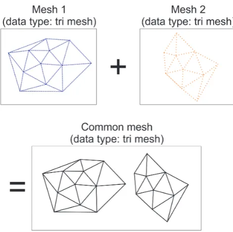
Abbildung 10: Multiple bodies’ triangle meshes are internally handled like a single mesh, thus allowing for easy implementation of mutual illumination or shadowing as well self-illumination (diffuse) e.g. in crater walls.
8
Examplary Applications
8.1
Example: Phobos
The Martian moonPhoboshas been illuminated, showing shadowing e.g. of crater floors, see fig. 11 and 12. The spatial resolution of this mesh is 49152 triangles, i.e. approximately 278 m average triangle edge length.
8.2
Mutual Shadowing
Figure 13 shows mutual shadowing of two spheres. The two spheres are assumed to have equal radii of approx. 1200 km (comparable to Pluto, see below) and are equally meshed with 2048 and 4096 nodes and triangles each, respectively. One sphere is located at (0,0,0), whereas the other is located at (−3000,1000,500), solar radiation is assumed to impinge from direction (1,0,0). The shadow of one sphere on the surface of the other is clearly visible, showing discretization artifacts at the border, though. Note that in general, small bodies or lunar surfaces are available in much higher resolution, see fig. 4.
The Pluto-Charon binary system has been considered as second example. Idealized positi-ons of Pluto and Charon have been assumed, i.e. both bodies on x axis, separated by the real average distance of 19596 km. Radii are 1187 km and 606 km for Pluto and Charon, respectively. Figure (10) shows the shadow casted by Charon on Pluto’s surface, assuming the sun in direction (1,0,0).
8.3
Illumination Statistic
Abbildung 11: Solar illumination of Martian moonPhobos[5], showing realistic shadowing e.g. of craters.
Fk(x)·Ttot = {t∈[0,∞[ : Ik(t)≤x} (14)
In other words, the irradiance on triangle patch #kis smaller than some levelxfor ”Fk(x)%”
(a)Phobos[5], solar radiation from left hand side.
(b) Phobos [5], solar radiation from front (directed into image plane).
(c) Phobos [5], solar radiation from right
hand side. (d)Phobos[5], solar radiation from bottom.
Abbildung 13: Shadowing of two spheres of radius 1200 km, each. Spheres are located at (0,0,0) and (−3000,1000,500), respectively. Direction to sun is (1m,0,0).
Abbildung 14: Shadowing of Pluto (right) by its largest moon Charon (left) during lunar eclipse (idealized). Both bodies are located on the x axis, coordinates: Pluto (0,0,0), Charon (19596,0,0), sun vector (1,0,0).
9
Validation
Abbildung 15: Cumulative distribution function for the irradiance at different points (tri-angle patches) onPhobos’ surface, relative toTtot being Phobos’ spin period, i.e. 7.65 h.
Shown isFk(x), see eq. (14) for five different triangles
Abbildung 16: Mininmal/maximal/average values for the irradiance at different points (tri-angle patches) onPhobos’ surface, relative toTtot being Phobos’ spin period, i.e. 7.65 h.
Note that a number of triangles near the north pole (ID aporox. 20000) is in permanent daylight. Assumed obliquity was zero.
For validation purposes, a number of images acquired by the DAWN Framing Camera FC2 (see figure 18 for basic parameters) has been utilized. Corresponding ephemerides and poin-ting parameters have been provided by the SPICE toolkit in version N00066, released April 2017 [13].
DAWN/Vesta survey data set, i.e. the mission phase covering overview pictures of 4 Vesta following the approach phase and followed by the high-altitude mapping orbit (HAMO) and low-altitude mapping orbit (LAMO) phase:
Time Mission Phase Jul 16, 2011 Vesta arrival Aug 11 – 31, 2011 Vesta survey phase
Sep 29, 2011 – Nov 2, 2011 Vesta first high altitude orbit (HAMO) Dec 12, 2011 – May 1, 2012 Vesta low altitude orbit (LAMO)
Jun 15, 2012 – Jul 25, 2012 Vesta second high altitude orbit (HAMO) Sep 5, 2012 Vesta departure
Tabelle 1: DAWN mission phases in Vesta’s vicinity.
During the survey phase, the average distance between the S/C and 4 Vesta is approx. 2720 km, phase angles (angle between line-of-sight DAWN-Vesta and line connecting Vesta and the sun) cover the range from approx. 11 deg to approx. 81 deg.
The image resolution is constant at 1024 x 1024 pixels. The Vesta shape model (compare section 4) is available in four different resolutions:
Resolution No. of triangles Average edge length coarse 49152 6744.7 m
medium 196608 419.2 m fine 786432 28.3 m super-fine 3145728 1.7 m
Tabelle 2: Available resolutions of surface grid of 4 Vesta.
Abbildung 18: Basic parameters of Framing Camera 2 of the DAWN mission [18]. For the study presented here, data of the camera #ID 2 have been utilized.
Abbildung 19: Filter settings of Framing Camera 2 of the DAWN mission [18]. For the study presented here, measurements using the clear filter have been utilized.
Abbildung 20: Left: Simulated image, right: real image as acquired by DAWN Framing Camera FC2. Image ID..
9.1
Statistical Analysis
Simulated and acquired images are compared by utilizing the irradiance probability density distribution (IPDF). Measured respectively simulated irradiances have been binned into 10 W/m2 bins ranging from 0 to approx. 290 W/m2. Note that the solar constant at 4 Vesta
(approx. 2.27 AU from the sun during the DAWN survey phase) is approximately 267 W/m2.
An examplary IPDF is shown in figure 22.
Abbildung 21: Left: Simulated image, right: real image as acquired by DAWN Framing Camera FC2. Image IDFC21B0005907-11232212051F1B.FIT.
Abbildung 22: Exemplary irradiance probability density function of image ID 11241023036. DAWN image acquired on August 31. The IPDF shows an average irradiance of approx. 151 W/m2and minimal and maximal values of 0. (black pixel or deep shadow) and 260 W/m2,
book level introduction. The test method is briefly outlined as follows. Assume a given IPDF with frequenciesf1, . . . , fn for the various irradiance bins. This is represented by the IPDF
of the measured image. Assumep1, . . . , pn be the frequencies of the IPDF to be compared
with. Given N samples pixels in this case), the deviation between the two IPDF can be quantified by theχ2
s value:
χ2s=
N X
k=1
(fk−N pk)2
N pk
(15)
Theχ2s test statistic is an overall measure of how close the observed frequencies fk are to
the expected frequencies pk. Obviously, the ’null hypothesis’ (PDF and independent, i.e.
simulated and measured image are not similar at all) is rejected ifχ2 is large, because this means that observed frequencies and expected frequencies are far apart. A quantification of ’large’ is acquired by theχ2 probability density function:
f(x) = x
N/2−1e−x/2
2N/2Γ(N/2) (16)
Here,N represents the degrees of freedom, identical with the number of pixels in our case. Theχ2curve is used to judge whether the calculated test statistic is large enough. We reject
the null hypothesis if the test statistic is large enough so that the area beyond is less than 0.05 :
P(χ2≥χ2s) =
Z ∞
χ2 s
f(χ2)d(χ2) (17)
This test is done for every picture and for every resolution available for the Vesta surface grid (see table 2). As can be seen in figures 23 - 26, the majority of the test cases yield values ofP(χ2 ≥χ2s)<0.05, i.e. the null hypothesis is rejected. Note that the null hypothesis is acutally that the underlying IPDF of the acquired and simulated images are different. Thus, the reliability of the algorithm is good.
Additionally, the quality of the simulated images, taking the number of test cases with
P(χ2 ≥χ2
s)<0.05 as metric - improves for increasing number of surface triangles. This is
reasonable, since the real surface can be considered as thenT =∞limit case and the effect
Abbildung 23: Results ofχ2test, 49152 surface triangles.
Abbildung 25: Results of χ2 test, 786432 surface triangles.
10
Conclusions and outlook
An efficient raytracing software for simulation of camera images as well as illumination conditions of small bodies as well as planetary surfaces has been implemented. Direct as well as indirect illumination as well as illumination of multiple bodies are possible. Different bidirectional reflectance functions are implemented. This includes the four-parameter Hapke model.
The illumination model has been validated using aχ2 statistical test to compare simulated images with a large number of DAWN acquired images. Good statistical match is found in general.
Main benefits of the simulation suite are its easy implementation and the option to use it as forward model in an inverse problem solver to derive optical properties of the surface of small bodies or planetary surfaces (without atmosphere).
Using this illumination model, optical parameters can be extracted from the comparison of simulated and observed radiances and applications of an optimization algorithm to those data. Images in different spectral bands can be easily computed by restriction of the solar spectrum to the spectral region under consideration. This way, dependence of the spectral parameters on wavelength can be examined.
[1] R. L. Cook and K. E. Torance. A relectance model for computer graphics. ACM Transactions on Graphics, 1(1), 1982.
[2] ESA. Asteroid impact mission: Didymos reference model. Technical Report 2.1, ESA, 2015.
[3] R. Gaskell, J. Saito, M. Ishiguro, T. Kubota, T. Hashimoto, N. Hirata, S. Abe, O. Barnouin-Jha, and D. Scheeres. Gaskell itokawa shape model v1.0. hay-a-amica-5-itokawashape-v1.0. NASA Planetary Data System, 2008.
[4] R.W. Gaskell. Gaskell eros shape model v1.0. near-a-msi-5-erosshape-v1.0. NASA Planetary Data System, 2008.
[5] R.W. Gaskell. Gaskell phobos shape model v1.0. vo1-sa-visa/visb-5-phobosshape-v1.0.
NASA Planetary Data System, 2011.
[6] C. M. Goral, K. E. Torrance, D. P. Greenberg, and B. Battaile. Modeling the interaction of light between diffuse surfaces. Computer Graphics, 18(3), 1984.
[7] E. Graciano, J. and. Chester. Autonomous rover path planning and reconfigurati-on. In 11th Symposium on Advanced Space Technologies in Robotics and Automation (ASTRA), European Space Agency, Noordwijk, Netherlands., 2011.
[8] B. W. Hapke. Bidirectional reflectance spectroscopy. J. Geophys. Res., 86:3039–3054, 1981.
[9] M. D. Hicks, B. J. Buratti, K. J. Lawrence, J. Hillier, J.-Y. Li, V. Reddy, S. Schr¨oder, A. Nathues, M. Hoffmann, L. le Corre, R. Duffard, H.-B. Zhao, C. Raymond, C. Russell, T. Roatsch, R. Jaumann, H. Rhoades, D. Mayes, T. Barajas, T.-T. Truong, J. Foster, and A. McAuley. Spectral diversity and photometric behavior of main-belt and near-Earth vestoids and (4) Vesta: A study in preparation for the Dawn encounter. Icarus, 235:60–74, June 2014.
[10] J. T. Kajiya. The rendering equation. InComm. ACM, SIGGRAPH 1986, volume 5-6, 1986.
[11] A. S. Konopliv, S. W. Asmar, R. S. Park, B. G. Bills, F. Centinello, A. B. Chamberlin, A. Ermakov, R. W. Gaskell, N. Rambaux, C. A. Raymond, C. T. Russell, P. Smith, D. E. Tricarico, and M. T. Zuber. The vesta gravity field, spin pole and rotation period, landmark positions, and ephemeris from the dawn tracking and optical data. Icarus, 240:103–117, 2013.
[12] J.-Y. Li, L. B. Le Corre, S. E. Schr¨oder, V. Reddy, B. W. Denevi, B. J. Buratti, M. Mottola, S. nd Hoffmann, P. Gutierrez-Marques, A. Nathues, C. T. Russell, and C. A.W. Raymond. Global photometric properties of asteroid (4) vesta observed with dawn framing camera. Icarus, 226(2):1252–1274, 2013.
[13] Navigation and Ancillary Information Facility (NAIF). Spice - an observation geometry system for space science missions. Technical report, National Aeronautics and Space Administration (NASA), 2017.
[14] Tompkins P., A. Stentz, and D. Wettergreen. Global path planning for mars rover exploration. In Proceedings of the 2004 IEEE Aerospace Conference, volume 1339, 2004.
[16] S. M. Parkes, I. Martin, and I. Milne. Lunar surface simulation – modelling for vision guided lunar landers. In Proc. DASIA, ESA Pub., 1999.
[17] V. Reddy, A. Nathues, L. C. Lucille, H. Sierks, J.-Y. Li, R. Gaskell, T. McCoy, A. W. Beck, S. E. Schr¨oder, C. M. Pieters, K. J. Becker, B. J. Buratti, B. Denevi, D. T. Blewett, U. Christensen, M. J. Gaffey, P. Gutierrez-Marques, M. Hicks, H. U. Keller, T. Maue, S. Mottola, L. A. McFadden, H. Y. McSween, D. Mittlefehldt, D. P. O’Brien, C. Raymond, and C. Russell. Color and albedo heterogenity of vesta from dawn.
Science, 336:700–703, 2012.
[18] H. Sierks, H. U. Keller, R. Jaumann, H. Michalik, T. Behnke, F. Bubenhagen, , I. B¨uttner, U. Carsenty, U. Christensen, R. Enge, B. Fiethe, P. Guti´errez Marqu´es, H. Hartwig, H. Kr¨uger, W. K¨uhne, T. Maue, S. Mottola, A. Nathues, K.-U. Reiche, M. L. Richards, T. Roatsch, S. E. Schr¨oder, I. Szemerey, and M. Tschentscher. The dawn framing camera. Space Science Reviews, 163:263–327, 2011.